Effective plant discrimination based on the combination of local binary pattern operators and multiclass support vector machine methods

Edith Cowan University

Edith Cowan University

Research Online

Research Online

ECU Publications Post 2013

1-1-2019

Effective plant discrimination based on the combination of local

Effective plant discrimination based on the combination of local

binary pattern operators and multiclass support vector machine

binary pattern operators and multiclass support vector machine

methods

methods

Vi Nguyen Thanh Le

Edith Cowan University, [email protected]

Beniamin Apopei

Edith Cowan University, [email protected]

Kamal Alameh

Edith Cowan University, [email protected]

Follow this and additional works at: https://ro.ecu.edu.au/ecuworkspost2013

Part of the Agriculture Commons

10.1016/j.inpa.2018.08.002

Nguyen Thanh Le, V., Apopei, B., & Alameh, K. (2019). Effective plant discrimination based on the combination of

local binary pattern operators and multiclass support vector machine methods. Information Processing in

Agriculture, 6(1), 116-131. Available

here.

This Journal Article is posted at Research Online.

https://ro.ecu.edu.au/ecuworkspost2013/5963

Effective plant discrimination based on the

combination of local binary pattern operators and

multiclass support vector machine methods

Vi Nguyen Thanh Le

, Beniamin Apopei

, Kamal Alameh

Edith Cowan University – Electron Science Research Institute, Australia

A R T I C L E I N F O

Article history:

Received 24 January 2018 Received in revised form 29 June 2018

Accepted 4 August 2018 Available online 10 August 2018

Keywords: Plant discrimination Classification LBP PCA and SVM A B S T R A C T

Accurate crop and weed discrimination plays a critical role in addressing the challenges of weed management in agriculture. The use of herbicides is currently the most common approach to weed control. However, herbicide resistant plants have long been recognised as a major concern due to the excessive use of herbicides. Effective weed detection tech-niques can reduce the cost of weed management and improve crop quality and yield. A computationally efficient and robust plant classification algorithm is developed and applied to the classification of three crops: Brassica napus (canola), Zea mays (maize/corn), and radish. The developed algorithm is based on the combination of Local Binary Pattern (LBP) operators, for the extraction of crop leaf textural features and Support vector machine (SVM) method, for multiclass plant classification. This paper presents the first investigation of the accuracy of the combined LBP algorithms, trained using a large dataset of canola, radish and barley leaf images captured by a testing facility under simulated field condi-tions. The dataset has four subclasses, background, canola, corn, and radish, with 24,000 images used for training and 6000 images, for validation. The dataset is referred herein as ‘‘bccr-segset”and published online. In each subclass, plant images are collected at four crop growth stages. Experimentally, the algorithm demonstrates plant classification accu-racy as high as 91.85%, for the four classes.

Ó2018 China Agricultural University. Production and hosting by Elsevier B.V. on behalf of KeAi. This is an open access article under the CC BY-NC-ND license (http://creativecommons. org/licenses/by-nc-nd/4.0/).

1.

Introduction

Weed infestation has always been a critical issue that limits the productivity of farms and the yield of crops. The ability

to accurately discriminate weeds from crops in real-time will advance precision crop and weed management, whereby weeds in a field are prevented from competing for light water and nutrients required by the crops. Blanket herbicide spray-ing is currently the most common practice used for weed con-trol. The worthwhile objective of precision weed control is to bring down the cost of weed management. To enhance the longevity of the current range of agricultural chemicals, it is important to deter the increase in herbicide resistant weeds. Cereal crops such as wheat, rice, maize (corn), oats, barley, rye and sorghum, represent a large portion of the crops grown worldwide [1]. Hence, detecting dominant weeds in cereal

https://doi.org/10.1016/j.inpa.2018.08.002

2214-3173Ó2018 China Agricultural University. Production and hosting by Elsevier B.V. on behalf of KeAi. This is an open access article under the CC BY-NC-ND license (http://creativecommons.org/licenses/by-nc-nd/4.0/).

* Corresponding author at: 270 Joondalup Drive, Joondalup, Western Australia, 6027, Australia.

E-mail addresses:[email protected](V. Nguyen Thanh Le), [email protected] (B. Apopei), [email protected]

(K. Alameh).

1 _{Address: 270 Joondalup Drive, Joondalup, Western Australia,}

6027, Australia.

Peer review under responsibility of China Agricultural University.

INFORMATION PROCESSING IN AGRICULTURE 6 (2019) 116–131

crop fields and controlling them in real-time will enable effec-tive site-specific weed management, resulting in substantial economic benefits[2]. A variety of weed detection approaches based on feature extraction have been proposed, these include shape-based analysis[3,4], colour-based analysis[5], texture-based image analysis [6,7] and spectral analysis

[8–10]. However, the accuracy of the above mentioned approaches has been limited due to the complexity of the field environment, the wide variety of species and the morphological variation of plants at various growth stages.

Numerous approaches to the discrimination of crops and weeds have been reported. Over the last two decades, spectral techniques based on the calculation of the Normalised Differ-ence Vegetation Indices (NDVIs)[11,12]have been proposed for distinguishing between plant species. However, these spectral techniques have some limitations, especially when the spectral characteristics of weeds and crops are similar over the operational wavelengths. In addition, in typical farm-ing field conditions, the wind, shadowfarm-ing, and background illumination may change the spectral features of plants, thus reducing the discrimination accuracy of NDVI-based weed sensors[13,14]. The limitations of such spectral-reflectance sensors have triggered research on the development of spatial sensors, based on the use of image processing techniques, for the classification of plant species and detection of weeds in real time.

A variety of feature extraction operators have been pro-posed for detecting robust features in images, based on the Scale Invariant Feature Transform (SIFT) [15], Speeded Up Robust Features (SURF)[16], the Histogram of Oriented Gradi-ents (HOG)[17], LBP, Gabor filters[18]to name a few. In this paper, we adopt the LBP technique for plant feature extraction for several reasons. Firstly, LBP method is very flexible and robust to monotonic grey-level transformation, illumination, scaling, viewpoint, and rotation variance [6]. Secondly, the LBP method enables image analysis in challenging real-time settings, due to computational simplicity [19]. In fact, the LPB is computationally less complex than its SIFT or SURF counterparts, exhibiting high discrimination capability [20]. Finally, the LBP has exhibited superior performance in several applications, such as face recognition[21–23], face expression analysis [24,25], texture classification [6,26,27], and motion analysis[28,29].

The optimization of LBP methods for discriminating crops and weeds has proved difficult in special scenarios[30,31]. In particular, Ahmed et al. used 400 colour images (taken at an angle of 45°with respect to the ground) in natural lighting conditions, 200 samples were of broadleaves and 200 of grass weeds[31]. From observation the number of images and the types of plants collected in the dataset is limited. Reduced accuracy was attained in the field due to the relatively small number of plant images and viewpoints, variable lighting conditions and change in plant aspect ratios for each growth stage. Furthermore, several extended LBP methods have used common and published texture databases including Outex

[32], Brodatz[33], UIUC[34], UMD[35]and CUReT[36]to vali-date, evaluate or compare classification results[37]. However, databases for the detection and classification of plant tex-tures have not been commonly published.

Typically, after extracting good features from plant images, the next process is to classify plant species. Previous research has mainly focused on the use of artificial neural networks (ANN) [38,39], Bayesian classifiers [40–42], k-nearest neigh-bour (KNN) classifiers[43], discriminant analysis[44,45]and SVM classifiers[46–49]for weed identification and discrimina-tion. According to[50–52], SVM has been regarded as a robust technique for difficult classification tasks. This paper focuses on applying the LBP method in conjunction with SVM for plant feature extraction and classification of various plants images.

The main contributions of the work in this paper are sum-marized as follows:

A large plant dataset was captured by using a Testbed with around 30,000 plant images. This large dataset contains four classes, a variety of plant images at four defined growth stages, with rotation, scale and viewpoint variance in order to evaluate the robustness and performance of the method.

Due to the low dimensionality of the plant representation and the low tolerance to illumination changes, LBP was especially investigated with different parameters for plant detection, and combined with SVM-based classification to investigate its capability to operate in real-time.

The paper consists of four sections and is structured as follows.Section 1explains why weed detection plays a cru-cial role in agricultural precision. It also introduces the selected method and presents a brief review of LBP analysis, together with the advantages and disadvantages of the pro-posed weed detection and classification approach.Section 2

describes the principles of the LBP technique and the ratio-nale of combining LBP operators with SVM for the extraction of key features from plant images and the classification of different types of plants in a large dataset. Performance measures for classification, data collection, and a detailed flowchart for training and validating the dataset are also covered in Section 2. InSection 3, an initial comparison of greyscale unsegmented and segmented images used in plant discrimination is provided. Results are presented in Sec-tion 3, indicating that performance is best achieved by using segmented images (i.e. working with the green plant mate-rial extracted from images and converting it to greyscale). Based on these initial results, the data set ‘‘bccr-segset”is collected in the form of greyscale segmented images. Then, the classification accuracy and F1 scores of groups with dif-ferent plant classes are discussed in detail, illustrating the effectiveness of the methodology in regard to plant detection and classification. Finally, conclusions and future work are discussed in Section 4.

2.

Materials and methods

This section describes the methodology and performance metrics that lead to the generation of the results shown in

Section 3. The theoretical concept and principle of the selected methods in segmentation, feature extraction and

classification processes are detailed inSections 2.1–2.3. Clas-sification accuracy and F1 scores measures are presented in

Section 2.4. Data collection is explained in detail in

Section 2.5.

2.1. Segmentation

Image segmentation refers to the process of partitioning an image into multiple segments or regions. In terms of weed detection, this process is based on the segmentation of green plant material (crops and weeds) and non-green background areas (i.e. soil and residues). Removing the background areas of the images enables better plant feature extraction and classification.

In this paper, the ExG-ExR (Excess Green minus Excess Red Indices) method is used to segment green plant regions. This colour index-based method has exhibited adequate robust-ness and high accuracy compared to other methods, such as ExG (Excess Green Index)+Otsu and NDI (Normalised Dif-ference vegetation Index)+Otsu under greenhouse field light-ing conditions and natural field lightlight-ing conditions [53]. Typically, the ExG component extracts green information, while the ExR component eliminates the background noise

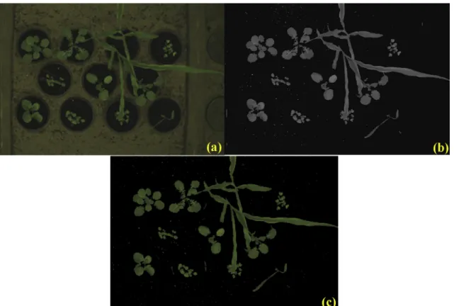
[54]. An example of image segmentation is illustrated in

Fig. 1, which shows canola, corn and radish plants that were randomly arranged along the testing trays of a test bed. The vegetation indices of the RGB plant image were first extracted by applying the ExG-ExR approach, then, the image was con-verted to a greyscale image before applying feature extraction and classification.

2.2. Local binary pattern operators

To better understand how LBP is applied for weed detection, a brief background on LBP is presented. The LBP method has been regarded as a powerful tool for extracting robust fea-tures from texture-based image analysis and classifying objects based on local image texture properties. The first LBP algorithm was reported in 1996[55], since then, various LBP algorithms have been developed to primarily detect tex-tures or objects in images. A very small local neighbourhood of a pixel is used to calculate a feature vector. Basically, the LBP operator labels the pixels of an image by thresholding the local structure around each pixel and considering the result as a binary number. Fig. 2 illustrates an example of computing LBP in a 33 neighbourhood by comparing the intensities of the eight neighbours around each pixel with the intensity of the centre pixel. When the intensity of the centre pixel is greater than that of a neighbour, it is consid-ered to be ‘0’, otherwise ‘1’. A binary chain is obtained by combining every single binary code in a clockwise direction. For Fig. 2, the binary code is 11110001, or 241 in decimal

[55]. The binary number is used to build a histogram, which can be regarded as representing the texture of an image.

The main limitation of the LBP operator presented above is that it only covers a small area of the neighbourhood. For a small 33 neighbourhood the LBP fails to capture dominant textural features in an image. As a result, the LBP operator was improved upon by increasing the number of pixels and the radius in the circular neighbourhood [6]. Note that it is typically more flexible and effective to improve LBP operators

Fig. 1 – Images of canola, corn and radish: (a) full RGB image, (b) image with extracted green material (plants), and (c) greyscale image of (b).

using textures of different scales. Generally, the value of the LBP code of a pixelðxc;ycÞcan be calculated as follows[6]:

LBPP;R¼ XP1 p¼0 sðg_pg_cÞ2p _{where s xð Þ ¼} 1; x0 0; x<0 ð1Þ where

g_c: is the grey value of the centre pixel.

g_p: represent the grey values of the circularly symmetric neighbourhood from p¼0 to P1 and g_p¼xP;R;p.

P: is the number of surrounding pixels in the circular neighbourhood with the radius R.

s xð Þ: is the thresholding step function which helps the LBP algorithm to gain illumination invariance against any monotonic transformation.

According to Eq.(1), the LBPP;Roperator produces 2P

differ-ent output values. If the image is rotated, the grey values, gp,

of the circularly symmetric neighbourhood will move corre-spondingly along the perimeter of the circle. This generates a different LBP value, except for patterns with only the value ‘0’ or ‘1’. In order to eliminate rotation effects, a rotation-invariant LBP is defined as follows[6]:

LBPri

P;R¼min ROR LBPð P;R;iÞ j i¼0;1; ;P1

ð2Þ where RORðx;iÞperforms an i-step circular bit-wise right shift on the P-bit number x.

To choose good and quality features, feature space dimen-sionality needs to be reduced by keeping only the rotationally-unique patterns. Accordingly, Ojala et al. named these patterns uniform patterns. The patterns denoted as LBPu2

P;Rstand for the number of spatial transitions in the

pat-terns meaning that the uniform patpat-terns need to have two bitwise transitions from 0 to 1 or vice versa. For instance, uni-form patterns with eight pixels in the circular neighbourhood, 00000000 (0 transitions), 11111111 (0 transitions), or 01110000 (2 transitions) are uniform because the parameter U that measures the uniformity has at most 2 transitions. Examples of non-uniform patterns are: 00000101 (4 transitions) and

01000101 (6 transitions). Consequently the rotation invariant uniform descriptor LBPriu2

P;R can be defined as follows[6]:

LBPriu2 P;R ¼ PP1 p¼0s xP;R;pxc ; if UðLBPP;RÞ 2 Pþ1; if UðLBPP;RÞ>2 ( ð3Þ

The uniform descriptor has PðP1Þ þ3 patterns including PðP1Þ þ2 distinct uniform patterns and all non-uniform patterns assigned to a groupðPþ1Þ. According to Ojala et al., the rotation invariant uniform descriptor hasðPþ2Þdistinct output patterns[6]. This reduces the feature space and helps increase the speed of LBP. For example, if the number of pixels in the circular neighbourhood is 8, the number of uniform patterns is 58 and the number of rotation invariant uniform patterns is 10.

2.3. Support vector machine

The final stage in the image processing is classification. There are different machine learning methods such as decision trees, SVM, neural networks, k-nearest neighbour method, and the Bayesian classifier. For a classifier to achieve good performance, sufficient data needs to be acquired and the training performance analysed. The SVM can deal with pat-tern classification and eliminate over-fitting, and it is robust to noise[47,56]. SVM was first introduced in 1992[57]. SVM performs classification more accurately than other algo-rithms in many applications, especially those applications involving very high dimensional data [42,46,47,58,59]. This high performance makes the SVM classifier a preferred option for many applications, such as face recognition, weed identi-fication and disease detection in plant leaves. Therefore, the optimal combination of the LBP descriptors and SVM classifi-cation can result in high plant discrimination accuracy. In particular, SVM generates an optimal hyper-plane that maxi-mizes the margin between the classes.

To be a good discriminative classifier, SVM needs to use an appropriate kernel function. Due to the separation of the learning algorithm and kernel functions, kernels can be stud-ied independently of the learning algorithm. One can design and experiment with different kernel functions without

Fig. 2 – An example of computing LBP codes. A binary code is obtained by comparing the intensity of the centre pixel with those of the eight neighbours in a 33 neighbourhood.

touching the underlying learning algorithm. Commonly, polynomial or Gaussian RBF (Radial Basis Function) kernels are used in most applications, depending on the types of data. In this paper, 2nd order polynomials and 5-fold cross validation are used. Specifically, the training set is firstly divided into five subsets of equal size, and four parts of the data are iteratively used for training, with the remaining part of data used for testing. This cross-validation procedure helps to prevent data overfitting and subsequent loss of generalization.

2.4. Performance metrics for plant classification

The common way of assessing a classification algorithm is to calculate its classification accuracy, which is defined as Classification Accuracyð Þ%

¼Number of correct classifications_{Total number of samples} 100% ð4Þ

However, in order to assess the performance of the SVM classifier for each class, confusion matrices are evaluated by computing main metrics, namely: precision, recall and F1 score, from the measured true positives, false positives, true negatives and false negatives. This method has been applied in many studied to evaluate the performance of classification models[60–62]. All parameters differentiate the correct classi-fication of labels within different classes[63,64]. A basic con-fusion matrix comprises 4 entries: True Positive (TP), False Negative (FN), False Positive (FP) and True Negative (TN). According to[64], we can calculate the average of precision, recall and F1 score for multi-class classification by firstly com-puting these parameters based on TP, TN, FN, and FP in each class as follows:

Recall ðclassÞ ¼_TPðclassTP_{Þ þ}ðclass_FNÞ_ðclassÞ ð5Þ

Precision ðclassÞ ¼_TPðclassTPð_{Þ þ}class_FPðÞ_classÞ ð6Þ

F1score ðclassÞ ¼2PrecisionðclassÞ RecallðclassÞ

PrecisionðclassÞ þRecallðclassÞ

¼_{2TPðclassÞ þ}2TP_FNð_ðclass_classÞ_{Þ þFPðclassÞ} ð7Þ

Precision in each class is defined as the number of cor-rectly classified positive plant images divided by the total number of plant images in the data. Recall in each class is the ratio of the number of correctly classified positive plant images to the number of positive plant images in the data. F1 score in each class is a composite measure of precision and recall in each class.

2.5. Data collection

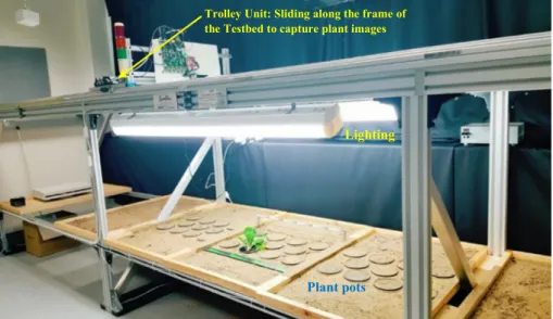
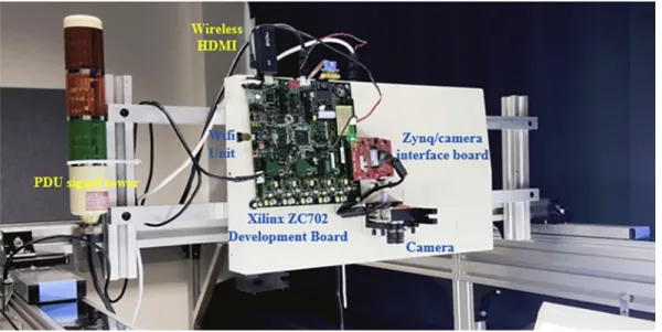
In this study all the data was captured on a custom-built test-ing facility at ESRI (Electron Science Research Institute), Edith Cowan University, Australia, which is shown inFigs. 3and4. The hardware comprises a Xilinx Zynq ZC702 development platform [65] that captures HD images (19201080 pixels) at 60 frames per second using an On-Semi VITA 2000 camera sensor. The Zynq development board and camera are mounted on a moveable trolley with the camera optical axis perpendicular to the ground and move on a linear drive across the frame of the Testbed. The captured images have a spatial resolution of 1mm/pixel and a size of 228228 pixels, which is down-sampled by a factor of 2 from a size of 456 456 pixels. In addition, the vertical height of the camera above the surface of the plant pots is 980 mm and 9 mm is the cam-era focal length.

As can be seen inFig. 3, individual trays are capable of holding 11 potted plants, with each tray filled with soil to pro-vide a uniform background that can be used to simulate a West Australian wheat belt farming environment. For experi-mental purposes, only the outer pot plant holders of the mid-dle tray were used.

The maximum allowable speed of the trolley is 5 m/s, with the system capable of capturing images in real-time. The Testbed is also equipped with two fluorescent tube lamps as

Plant pots Lighting

Trolley Unit: Sliding along the frame of the Testbed to capture plant images

illustrated inFig. 3. The artificial lighting is there to provide uniform illumination for the purposes of data capture. For the purposes of the experimental work presented herein, all data was captured at a speed of 1 m/s (3.6 km/h) to capture high quality images.

Data capture runs comprised collecting multiple images of the individual test plants placed in the centre Testbed tray,

Fig. 3, with image variation obtained through manual plant rotation. The segmented greyscale images collectively formed the large data set used in the experimental work. This data set is referred to herein as ‘‘bccr-segset”and published online.

2.5.1. Data labelling

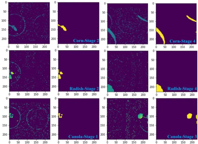
Data labelling was conducted by providing the ground truth in regard to which types of plants were identified in images. In the context of continuous runs on the Testbed, images com-prised just back ground, partial plant with background or full plant with background, making the detection and classifica-tion processes challenging. Whilst the partial plant images could be removed from the dataset altogether, this would introduce a dataset bias. On the other hand, the human label-ling error was quite high when attempts were made to decide among the labels that contained little plant information (i.e. ‘‘is this background or plant?”). Therefore, a semi-automatic way was adopted to solve this problem by thresholding the amount of green plant material according to their growth stages. If an image did not contain enough green plant mate-rial, then it was labelled as background.

First of all, as a pre-processing stage, images were filtered by using open and close morphological operations in order to remove the background noise. Then, binary images were seg-mented and thresholded according to the amount of corre-sponding plant area found. Initial experiments showed that it was not sufficient to do a green threshold on the entire image, therefore images were divided into 7 equal areas (Top left, Top right, Bottom left and Bottom Right, Centre left, Centre and Centre right) as shown inFig. 5.

The thresholding test was applied for each of the square areas shown inFig. 5. The image was labelled as a plant class

if the thresholding test passed for any of the areas. Lastly, an edge area threshold was also defined in order to allow for par-tial plants to have enough green material for identification. All the thresholds were experimentally derived and are shown inTable 1.

As can be seen in Fig. 6, partial plants in some growth stages with insufficient information were considered as a background class in the dataset. This allowed a more reliable labelling process without removing images from the dataset. In turn, this assured that the input sample distribution did not change.

2.6. Methodology

All of the plant images went through the following processing steps: pre-processing, segmentation, feature extraction and classification. The extracted LBP features were stored in a database. Pre-processing was the same for both training and

Fig. 4 – Zynq board with integrated VITA 2000 camera mounted on a moveable trolley.

Fig. 5 – Thresholding areas used in collected images to filter partial plants with insufficient information for

classification.

validation phases. The training dataset was trained by using the SVM and then the prediction model was exported to com-pare with textural features in the validation set for recognis-ing and classifyrecognis-ing different types of plants.

Steps in the process of the training, testing and validation of the dataset through the combination of LBP operators and SVM for three-plant classification are summarised as follows:

1. The dataset with greyscale segmented images is provided to start the process.

2. To read all plant images, the location of the dataset is input.

3. The dataset is divided into the training and validation phases.

4. The LBP hyper-parameters are set, including the number of neighbours (P) and the radius (R), and a rotation invari-ant uniform (riu2) descriptor. In the preliminary results,

LBPriu2 8;1, LBP

riu2 16;2, LBP

riu2

24;3 and combined LBP operators

LBPriu2

8;1þLBP16riu;22þLBPriu24;23

are applied to extract robust fea-tures from plant images.

5. The LBP method is initialised by inputting hyper-parameters then run to extract features from plant images.

6. Canola, Corn, Radish and Background are labelled by using the Testbed system in the data collection stage. For this step, a table of features and labels is generated to input into Matlab to train the dataset by using the LBP algorithm and SVM classifier.

7. The table of robust features and labels is regarded as an input dataset for training.

8. Apply the SVM approach with 5-fold cross validation to classify different types of plants. After training the data-set, a model is exported to make predictions for the plant images in a validation dataset.

Table 1 – Default thresholds for canola, corn and radish plants.

Thresholds for plants (cm2) Stage 1 Stage 2 Stage 3 Stage 4 Threshold (Inner, Edge)–Canola (1.4, 3.3) (3.0, 6.7) (7.0, 10.0) (8.0, 12.2) Threshold (Inner, Edge)–Corn (2.2, 5.7) (3.0, 6.7) (4.2, 9.2) (7.5, 13.9) Threshold (Inner, Edge)–Radish (2.5, 4.0) (3.2, 6.7) (7.0, 10.0) (8.0, 13.8)

Corn-Stage 2

Corn-Stage 4

Radish-Stage 2

Radish-Stage 4

3

e

g

a

t

S

-a

l

o

n

a

C

1

e

g

a

t

S

-a

l

o

n

a

C

Fig. 6 – Examples of filtered and segmented images of 3 different partial plants (Canola, Corn and Radish) removed from the dataset at three different growth stages.

9. The classification accuracy and F1 score are calculated. When other hyper-parameters are to be tested, this model is restarted at step 4.

3.

Results and discussion

The results are divided into two sections: (i) the accuracies of classification models are evaluated based on comparing an unsegmented validation dataset with a validation segmented dataset, and (ii) the classification accuracy of the LBP opera-tors and the SVM in the large dataset is reported. As noted in the data collection section, plant images were captured at the same height from the camera to the plant pots. Therefore, the scales of the images of the plants taken during the four growth stages corresponded to the actual sizes of the plants. The computer used in these experiments had a 3.4 GHz pro-cessor, 16 GB RAM and ran MATLAB 2016b.

3.1. Initial results of the comparison between classification accuracies of an unsegmented dataset and a segmented dataset

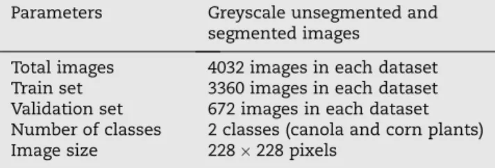
In this section, an initial performance comparison is made between segmented and unsegmented greyscale images. With regard the current experimental setup, the effort required to capture and label the unsegmented greyscale images is greater than that of capturing segmented images. Experiments are conducted by selecting unsegmented and segmented datasets with 4032 images in each dataset. The detailed parameters of the two datasets are listed inTable 2.

All plant samples consisted of canola and corn species taken, as previously mentioned, at three growth stages. The number of canola samples was equal to the number of corn samples in the training sets and the validation sets. Typical plant images in the unsegmented and segmented dataset for three different growth stages are shown inFig. 7.

The results of the classification accuracy were assessed against the percentages of correct classified plants. It can be observed fromTable 3that the combination of LBP operators significantly improves the classification accuracies in the val-idation sets. According to Ojala et al., the performance of the combined LBP operators outperformed that of single LBP operators[6]. In this experiment, it was obviously true that the classification accuracies achieved using the combination of LBPriu8;12, LBP

riu2

16;2 and LBP

riu2

24;3 was also higher than those

attained using single LBP operators. This demonstrates that robust features extracted through the combined-LBP opera-tors can increase the classification accuracy and F1 scores. In comparison with using the greyscale unsegmented dataset, the accuracy of classification models using the validation seg-mented dataset is generally higher.

The experimental results shown inTable 3show that con-verting RGB plant images into greyscale without segmenta-tion does not increase the classificasegmenta-tion accuracy. Whereas, by segmenting RGB images using the ExG-ExR method and then converting them to greyscale results in higher classifica-tion accuracy. Furthermore, experimental results show that by applying the above-mentioned pre-segmentation steps an increase of 2–4% in accuracy is attained, for the detection and discrimination of plant species.

Principal Component Analysis (PCA) is a useful tool for reducing the dimensionality of data. Typically, PCA produces the principal components of an image and extracts the rele-vant features from the data matrix of the image by calculating the eigenvalues. Note, however, in some cases, many signifi-cant features could be eliminated when PCA is applied, thereby reducing plant discrimination accuracy [66,67]. Therefore, optimising the number of retained principal com-ponents is important for increasing plant discrimination accuracy. In our experiments, PCA was used in conjunction with the combined-LBP operators and SVM, and the optimum number of principal components for our algorithms was

Table 2 – Parameters of unsegmented and segmented datasets.

Parameters Greyscale unsegmented and segmented images

Total images 4032 images in each dataset Train set 3360 images in each dataset Validation set 672 images in each dataset Number of classes 2 classes (canola and corn plants) Image size 228228 pixels

Fig. 7 – Greyscale unsegmented (a) and segmented (b) plant images at three different growth stages of canola and corn plants.

found to be 16. This optimum number was deduced experi-mentally and is offered herein for completion.

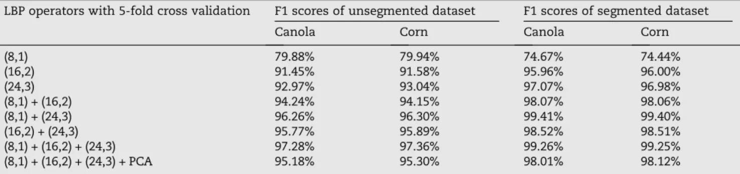
Note that classification accuracy is not a sufficient indica-tor to claim that the model is acceptable for plant classifica-tion [63]. In fact, three other indicators (Precision, Recall, and F1 score) are typical to validate the suitability of the model for plant classification.Table 4shows the F1 scores of the classification models for the validation unsegmented and validation segmented datasets, for canola and corn plants. As seen fromTable 4, the F1 scores for canola and corn plants are relatively similar. It is obvious fromTable 4that the highest F1 scores (>99%) are attained with segmented data and the combination of LBPriu2

8;1 and LBP riu2 24;3.

3.2. Classification accuracies and F1 scores of a multi-class dataset

Having investigated the performance of the greyscale seg-mented images (in Section 3.1), we discuss in this section the performance of the method based on the combination of the LBP operators and SVM for a larger dataset, using only greyscale segmented images.

In these experiments canola, corn and radish plants were collected at four different growth stages, Fig. 8, using the custom-built testbed. Images were segmented and converted to greyscale with the size of 228228 pixels. The datasets were divided into training and validation, as illustrated in

Fig. 9.

The training dataset was used to train the SVM classifier with 5-fold cross validation to generate a prediction model for the validation dataset. Kernel functions were introduced

to enhance efficient non-linear classification. Note that poly-nomial kernels and radial basis functions are widely used with SVM [68]. Different kernels were trialled in the experi-ments with the quadratic kernel was found to be more effec-tive for SVM and LBP combination, the quadratic kernel generating the best and most consistent results. The ‘‘one against one”SVM strategy was selected in this scenario due to the large number of training images [69]. This obtained the optimum compromise between training time and accu-racy performance. MATLAB was used to visualize the distribu-tion of the LBP textural features.

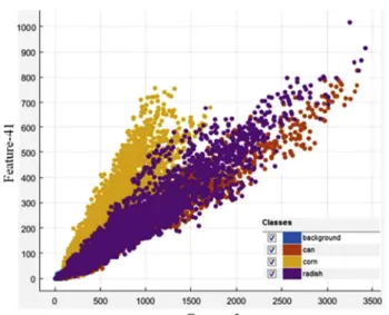
Fig. 10shows the distribution of the training dataset for canola, corn, radish and background, using LBP operators

LBPriu28;1; LBP riu2 16;2; LBP riu2 24;3

and the SVM classifier. The scatter plot shown in Fig. 10 illustrates the distribution of two selected features out of a total of 54 features. From the plant images, it is obvious that the texture of the corn leaves is completely different to that of the leaves of canola and radish. Corn is categorised as a narrow leaf plant, whilst canola and radish are broad leaf plants. The distributions of canola and radish plant features overlap, mainly because their measured textural features are similar, making their discrimination challenging. Intuitively, these plants have the same botanical family (Brassicaceae or Cruciferae) and corn belongs to grass family (Poaceae). However, this plot is limited by the distribu-tion of 2 selected features.

In order to visualize the structure of the ‘‘bccr-segset”large dataset in a two-dimensional map, we used t-SNE technique

[70]for the train dataset (24,000 plant images) and test dataset (6000 plant images). According to[70], as well as the user’s guide for t-SNE, we implemented this technique in Matlab,

Table 3 – Classification accuracies attained by using LBP operators with SVM for two different validation datasets.

LBP operators with 5-fold cross validation Number of bins Unsegmented dataset accuracy Segmented dataset accuracy

(8,1) 10 79.91% 75.45% (16,2) 18 91.52% 95.98% (24,3) 26 93.01% 97.02% (8,1) + (16,2) 28 94.20% 98.07% (8,1) + (24,3) 36 96.28% 99.40% (16,2) + (24,3) 44 95.83% 98.51% (8,1) + (16,2) + (24,3) 54 97.32% 99.26% (8,1) + (16,2) + (24,3) + PCA 16 95.24% 98.07%

Table 4 – F1 scores of the classification models for the validation unsegmented and validation segmented datasets.

LBP operators with 5-fold cross validation F1 scores of unsegmented dataset F1 scores of segmented dataset Canola Corn Canola Corn

(8,1) 79.88% 79.94% 74.67% 74.44% (16,2) 91.45% 91.58% 95.96% 96.00% (24,3) 92.97% 93.04% 97.07% 96.98% (8,1) + (16,2) 94.24% 94.15% 98.07% 98.06% (8,1) + (24,3) 96.26% 96.30% 99.41% 99.40% (16,2) + (24,3) 95.77% 95.89% 98.52% 98.51% (8,1) + (16,2) + (24,3) 97.28% 97.36% 99.26% 99.25% (8,1) + (16,2) + (24,3) + PCA 95.18% 95.30% 98.01% 98.12%

and used the main parameters, such as two-dimensional visualization, dimensionality reduction of the data (the value was 50), perplexity of the Gaussian distributions (the value was 30). Fig. 11 shows (a) the train dataset (24000 plant images) and (b) the test dataset (6000 plant images) with 4 classes (background, canola, corn and radish). As can be seen from Fig. 11, the distribution of background class is totally separated from other classes. Meanwhile, the distributions of corn, canola and radish images were classified into many small groups and had some overlapping patterns, leading to higher misclassification rates among canola, corn and radish images.

For the validation set, the generated prediction model was applied to evaluate the robustness of this model by evaluating the classification accuracies for scenarios of two classes, three classes and four classes. To evaluate the quality of clas-sification of the model, we applied performance measures to calculate the confusion matrices described inSection 2.4.

Performance metrics for multi-class classification were computed by applying the general formulas from Sokolova and Lapalme[64]. After training the 24000-plant-image data-set,Table 5shows the average classification accuracy results obtained on the test dataset (6000 plant images) by using the combination LBP operators LBPriu2

8;1; LBP riu2 16;2; LBP riu2 24;3 with PCA (16 principle components) and without PCA. The classifi-cation accuracy of LBP operators without PCA shown inTable 5

was relatively higher than the one with PCA. However, a slight improvement in execution time was obtained by applying PCA, due to reduction of features considered to 16 dominant features.

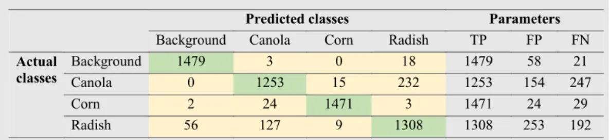
To have a better understanding of classification for classes,

Table 6shows the confusion matrix of the test dataset for four classes which was obtained by using SVM (polynomial kernel, order 2) without PCA. After calculating the number of cor-rectly and falsely classified images in the confusion matrix,

Fig. 8 – Segmented greyscale images of canola, corn and radish, at four different growth stages.

Fig. 9 – Illustration of the partitioning of the big dataset into training and validation datasets for canola, corn, radish and background.

TP, FP and FN parameters in each class were calculated. We applied performance measures to calculate the confusion matrix, precision, recall and F1-score of the test dataset

described inSection 2.4by using the SVM classifier (polyno-mial kernel, order 2) were computed as shown inTable 7.

The evaluation of the performance of different SVM ker-nels is presented in Table 7. According to a comparison of the F1 scores for multi-class classification, the classification performance of SVM (polynomial kernel, order 2, box con-straint level: 1) with 91.83% was higher than SVM (polynomial kernel, order 3, box constraint level: 1) and SVM (RBF kernel, box constraint level: 1, and kernel scale:

p

number of features

ð Þ) with 90.66% and 90.78% respectively. Furthermore, corn and background classes were classified with high accuracy. In contrast, for groups with many similar features (canola and radish), the algorithm displayed reduced discrimination capability.

The distinctions in the leaf texture of plants and the num-ber of green pixels in images provided significant information for the reliability of classification results. In particular, the dif-ferences between narrow-leaf and broadleaf plants enhanced the classification rates. Therefore, background and corn images were classified with higher accuracy compared to canola and radish images. As for the similarity between canola and radish plants, the F1 scores of differentiating between them in Table 7 were considerably lower. These plants with round shaped leaves can be discriminated by sim-ply recognizing the edges of canola plants, which generally look like outward-pointing teeth. In addition, one of the main obstacles for the relatively high misclassification rates is that

Table 5 – Classification accuracies of an algorithm combining LBP operators LBPriu2

8;1; LBPriu216;2; LBPriu224;3

and SVM for different scenarios. Execution time and PCA is shown herein for completion.

LBP operators with 5-fold cross validation

Average classification accuracy of LBP operators (8,1) + (16,2) + (24,3) Execution time (milliseconds/Image)

Average classification accuracy of LBP operators (8,1) + (16,2) +

(24,3) with PCA (16 principle components)

Execution time (milliseconds/ Image)

Four classes (Canola, Corn, Radish & Background)

91.85% 47.898 91.08% 45.418

Fig. 11 – Visualization of (a) the train dataset (24,000 plant images) and (b) the test dataset (6000 plant images) with 4 classes (background, canola, corn and radish).

Fig. 10 – Typical textural feature distribution of the training dataset for canola, corn, radish and background. Based on the LBP operators LBPriu2

8;1; LBPriu216;2; LBPriu224;3

and the SVM classifier. Textural feature distribution is shown for two selected features out of a total of 54 features.

plant leaves may look unexpectedly deformed and twisted after imaging, since these plants are not always perpendicu-lar to the camera lens. Overall, the algorithm combining LBP operators with SVM produced consistently robust classifica-tion, scale and rotation invariance.

To investigate the performance of SVM kernels, we con-ducted a comparative study of the F1 scores for SVM classifier and K-Nearest Neighbour (KNN) classifier. KNN is an algo-rithm for classifying classes based on a similarity measure (distance functions)[71]. This method has two types of dis-tance functions including disdis-tance metric and disdis-tance weight [72]. Particularly, three distance metrics including Euclidean, Minkowski and Cosine were used in this experi-ment and the results were computed by using Matlab.Table 8

shows the Precision, Recall and F1-score of the test dataset for different types of KNN. It is obvious fromTable 8 that the average F1 score in the case of using weight KNN (86.73%) was higher than other KNN techniques such as Coarse KNN (82.67%), Cosine KNN (83.79%), Fine KNN (85.78%), Cubic KNN (86.26%) and Medium KNN (86.50%). Based on the results shown inTables 7and8, the SVM classifier outperformed the KNN classifier for the test dataset (6000 images).

We used the dataset with four-growth stages, where leaves in each stage were captured with the difference of size and morphology. However, the number of collected images as

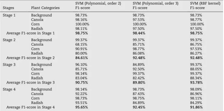
mentioned inFig. 9was not equal in each stage. In order to evaluate the performance of the classification of 4 different plant classes in each stage, we divided and equalised the train dataset (3200 plant images with 800 images in each class) and the test dataset (320 images with 80 images in each class). In addition, the effectiveness of the classified plant images was evaluated by the F1-scores in the case of three different SVM kernels. As can be observed inTable 9, the F1 score at stage 1 was higher than those at other stages. The morphology of canola and radish in stage 1 is distinctly different. Specifically, the two-heart shape of radish leaves in stage 1 has a distinc-tive appearance compared to the shape of canola leaves. As for the stage 2 and 3, the classification performance of SVM (RBF kernel) was higher than of SVM (polynomial kernel, order 2 and 3). However, the number of correctly classified plant images based on the F1 score was higher for the SVM (polynomial kernel, order 2) in comparison with the SVM (RBF kernel).

The capability of discriminating between canola and rad-ish images inTable 9was always lower than for background and corn images. Consequently, improving the LBP method is crucial to discriminate plant species with relatively similar features. A possible way to achieve this is to combine the uni-form rotation invariant LBP features with significant non-uniform LBP features. Another potential approach is to take

Table 7 – Precision, Recall and F1-score of the test dataset with different SVM kernels.

SVM kernels Train the dataset Classes Precision Recall F1-score Quadratic SVM 95.20% ± 0.25 Background 96.23% 98.60% 97.40%

Canola 89.05% 83.53% 86.21% Corn 98.39% 98.07% 98.23% Radish 83.79% 87.20% 85.46% The average of parameters 91.87% 91.85% 91.83%

Cubic SVM 96.00% ± 1.11 Background 96.41% 98.33% 97.36% Canola 86.59% 82.20% 84.34% Corn 98.04% 96.93% 97.49% Radish 81.77% 85.20% 83.45% The average of parameters 90.70% 90.67% 90.66%

RBF kernel 94.90% ± 0.37 Background 96.17% 98.87% 97.50% Canola 83.64% 85.20% 84.41% Corn 98.64% 96.87% 97.75% Radish 84.69% 82.27% 83.46% The average of parameters 90.79% 90.80% 90.78%

Table 6 – The number of plant images in the test dataset correctly and incorrectly recognized using the confusion matrix, for a group of three plants (canola, corn and radish) and background.

Table 8 – Precision, Recall and F1-score of the test dataset with different types of KNN.

KNN Classes Precision Recall F1-score

Fine KNN Background 95.75% 96.20% 95.98% Number of neighbours:1 Canola 77.37% 76.80% 77.08% Distance metric: Euclidean Corn 96.98% 91.93% 94.39% Distance metric: Equal Radish 73.70% 77.73% 75.67% The average of parameters 85.95% 85.67% 85.78%

Medium KNN Background 96.11% 98.87% 97.47% Number of neighbours:10 Canola 74.10% 83.93% 78.71% Distance metric: Euclidean Corn 96.65% 92.40% 94.48% Distance metric: Equal Radish 80.36% 70.93% 75.35% The average of parameters 86.81% 86.53% 86.50%

Coarse KNN Background 95.55% 98.80% 97.15% Number of neighbours:100 Canola 66.56% 81.33% 73.21% Distance metric: Euclidean Corn 95.50% 89.20% 92.24% Distance metric: Equal Radish 76.05% 61.60% 68.07% The average of parameters 83.42% 82.73% 82.67%

Cosine KNN Background 85.31% 99.13% 91.71% Number of neighbours:10 Canola 77.69% 72.67% 75.09% Distance metric: Cosine Corn 95.80% 88.13% 91.81% Distance metric: Equal Radish 77.20% 75.87% 76.53% The average of parameters 84.00% 83.95% 83.79%

Cubic KNN Background 96.05% 98.80% 97.40% Number of neighbours:10 Canola 73.52% 83.87% 78.36% Distance metric: Minkowski Corn 96.58% 92.13% 94.30% Distance metric: Equal Radish 80.23% 70.33% 74.96% The average of parameters 86.60% 86.28% 86.26%

Weighted KNN Background 96.11% 98.87% 97.47% Number of neighbours:10 Canola 76.05% 80.67% 78.29% Distance metric: Euclidean Corn 96.54% 93.07% 94.77% Distance metric: Squared inverse Radish 78.52% 74.33% 76.37% The average of parameters 86.81% 86.74% 86.73%

Table 9 – Precision, Recall and F1-score of the test dataset at four-growth stages with different SVM kernels.

SVM (Polynomial, order 2) SVM (Polynomial, order 3) SVM (RBF kernel) Stages Plant Categories F1-score F1-score F1-score

Stage 1 Background 98.73% 98.73% 98.73%

Canola 98.16% 97.53% 98.77%

Corn 100.00% 100.00% 100.00%

Radish 98.11% 97.50% 97.50%

Average F1-score in Stage 1 98.75% 98.44% 98.75%

Stage 2 Background 99.37% 99.37% 99.37%

Canola 68.15% 85.71% 86.75%

Corn 90.91% 98.77% 97.53%

Radish 80.00% 86.08% 86.27%

Average F1-score in Stage 2 84.61% 92.48% 92.48%

Stage 3 Background 96.10% 84.89% 99.37%

Canola 85.71% 92.50% 88.05%

Corn 98.14% 99.37% 99.37%

Radish 83.04% 82.42% 88.34%

Average F1-score in Stage 3 90.75% 89.80% 93.78%

Stage 4 Background 98.14% 98.73% 98.09%

Canola 92.22% 87.43% 86.96%

Corn 98.73% 98.75% 98.11%

Radish 93.51% 84.89% 84.29%

all features of the LBP method to acquire vital information of microscopic images of the plant species [73]. These are promising approaches that enable the development of LBP algorithms for the discrimination of plant species of similar features.

4.

Conclusions & future work

An algorithm based on the combination of LBP operators and an SVM classifier has been investigated, and its performance experimentally evaluated for the discrimination of different types of plants. An initial comparison of unsegmented and segmented dataset types has been carried out in order to identify the type that yields higher classification accuracy. This comparison has shown that the green segmentation pre-processing step is beneficial for feature extraction and classification. A large segmented dataset has been collected using a high-speed Testbed that enabled the methods to be assessed and validated. A dataset has been made available (published online), which can be flexibly used by other researchers for information and comparison. Particularly, eight cases have been created using the large dataset and the experimental results have demonstrated that the com-bined LBP algorithm can attain a discrimination accuracy greater than 91% for corn, canola and radish plants and back-ground. Results have also shown that if the shapes of canola and radish leaves are similar, the classification accuracy of the LBP algorithm decreases significantly. Furthermore, results have shown that the current execution time of plant classification is short, making the combined LBP algorithm a promising candidate for real-time weed detection.

Future work is focusing on the extension of the LBP method using colour images (instead of grey-level) and the introduction of identification techniques based on the use of non-uniform patterns in order to increase the weed detec-tion accuracy. In addidetec-tion, further investigadetec-tions are required for improving the classification of broad leaves (e.g., radish and canola) and assessing the LBP algorithm in scenarios in which weeds and crops are partially occluded.

Conflict of interest

The authors declared that there is no conflict of interest.

Acknowledgments

The research was funded by Grains Research and Develop-ment Corporation (GRDC) and the authors would like to thank the Pawsey Supercomputing Centre for storing the large dataset.

R E F E R E N C E S

[1]Leff B, Ramankutty N, Foley JA. Geographic distribution of major crops across the world. Global Biogeochem Cycl 2004;18(1):1–27.

[2]DiTomaso JM. Invasive weeds in rangelands: species, impacts, and management. Weed Sci 2000;48(2):255–65.

[3]Perez A, Lopez F, Benlloch J, Christensen S. Colour and shape analysis techniques for weed detection in cereal fields. Comput Electron Agric 2000;25(3):197–212.

[4]Søgaard HT. Weed classification by active shape models. Biosyst Eng 2005;91(3):271–81.

[5]Woebbecke D, Meyer G, Von Bargen K, Mortensen D. Color indices for weed identification under various soil, residue, and lighting conditions. Trans ASAE 1995;38(1):259–69. [6]Ojala T, Pietikainen M, Maenpaa T. Multiresolution gray-scale

and rotation invariant texture classification with local binary patterns. IEEE Trans Pattern Anal Mach Intell 2002;24 (7):971–87.

[7]Liu L, Lao S, Fieguth PW, Guo Y, Wang X, Pietika¨inen M. Median robust extended local binary pattern for texture classification. IEEE Trans Image Process 2016;25(3):1368–81. [8]Tang L, Tian L, Steward B, Reid J. Texture-based weed

classification using Gabor wavelets and neural network for real-time selective herbicide applications. Urbana

1999;51:61801.

[9]Ishak AJ, Hussain A, Mustafa MM. Weed image classification using Gabor wavelet and gradient field distribution. Comput Electron Agric 2009;66(1):53–61.

[10] Bossu J, Ge´e C, Jones G, Truchetet F. Wavelet transform to discriminate between crop and weed in perspective agronomic images. Comput Electron Agric 2009;65(1):133–43. [11] Hansen P, Schjoerring J. Reflectance measurement of canopy

biomass and nitrogen status in wheat crops using normalized difference vegetation indices and partial least squares regression. Remote Sens Environ 2003;86(4):542–53. [12] Thorp K, Tian L. A review on remote sensing of weeds in

agriculture. Precis Agric 2004;5(5):477–508.

[13] Huete A, Didan K, Miura T, Rodriguez EP, Gao X, Ferreira LG. Overview of the radiometric and biophysical performance of the MODIS vegetation indices. Remote Sens Environ 2002;83 (1):195–213.

[14] Ozdogan M, Yang Y, Allez G, Cervantes C. Remote sensing of irrigated agriculture: opportunities and challenges. Remote Sens 2010;2(9):2274–304.

[15] Lowe DG. Distinctive image features from scale-invariant keypoints. Int J Comput Vision 2004;60(2):91–110.

[16] Bay H, Ess A, Tuytelaars T, Van Gool L. Speeded-up robust features (SURF). Comput Vision Image Understand 2008;110 (3):346–59.

[17] Dalal N, Triggs B. Histograms of oriented gradients for human detection. In: IEEE computer society conference on computer vision and pattern recognition, 2005, CVPR 2005. IEEE; 2005. p. 886–93.

[18] Liu C, Wechsler H. Gabor feature based classification using the enhanced fisher linear discriminant model for face recognition. IEEE Trans Image Process. 2002;11(4):467–76. [19] Happy S, George A, Routray A. A real time facial expression

classification system using local binary patterns. In: 4th International conference on intelligent human computer interaction (IHCI). IEEE; 2012. p. 1–5.

[20] Lahdenoja O, Poikonen J, Laiho M. Towards understanding the formation of uniform local binary patterns. ISRN Mach Vision 2013;2013.

[21] Ahonen T, Hadid A, Pietikainen M. Face description with local binary patterns: application to face recognition. IEEE Trans Pattern Anal Mach Intell 2006;28(12):2037–41.

[22] Jin H, Liu Q, Lu H, Tong X. Face detection using improved LBP under Bayesian framework. In: Third international

conference on image and graphics (ICIG’04). IEEE; 2004. p. 306–9.

[23] Louis W, Plataniotis KN. Co-occurrence of local binary patterns features for frontal face detection in surveillance applications. EURASIP J Image Video Process 2010;2011(1): 745487.

[24]Zhao G, Pietikainen M. Dynamic texture recognition using local binary patterns with an application to facial expressions. IEEE Trans Pattern Anal Mach Intell 2007;29:6.

[25]Shan C, Gong S, McOwan PW. Facial expression recognition based on local binary patterns: a comprehensive study. Image Vis Comput 2009;27(6):803–16.

[26]Guo Z, Zhang L, Zhang D. A completed modeling of local binary pattern operator for texture classification. IEEE Trans Image Process 2010;19(6):1657–63.

[27]Liao S, Law MW, Chung AC. Dominant local binary patterns for texture classification. IEEE Trans Image Process 2009;18 (5):1107–18.

[28]Heikkila M, Pietikainen M. A texture-based method for modeling the background and detecting moving objects. IEEE Trans Pattern Anal Mach Intell 2006;28(4):657–62.

[29]Kellokumpu V, Zhao G, Pietika¨inen M. Human activity recognition using a dynamic texture based method. BMVC 2008;1:2.

[30]Ahmed F, Bari AH, Shihavuddin A, Al-Mamun HA, Kwan P. A study on local binary pattern for automated weed

classification using template matching and support vector machine. In: 12th International symposium on

computational intelligence and informatics (CINTI). IEEE; 2011. p. 329–34.

[31]Ahmed F, Kabir MH, Bhuyan S, Bari H, Hossain E. Automated weed classification with local pattern-based texture descriptors. Int Arab J Inf Technol 2014;11(1):87–94. [32]Ojala T, Maenpaa T, Pietikainen M, Viertola J, Kyllonen J,

Huovinen S. Outex-new framework for empirical evaluation of texture analysis algorithms. In: Proceedings of the 16th international conference on pattern recognition. IEEE; 2002. p. 701–6.

[33]Brodatz P. Textures: a photographic album for artists and designers. Dover Pubns; 1966.

[34]Lazebnik S, Schmid C, Ponce J. A sparse texture

representation using local affine regions. IEEE Trans Pattern Anal Mach Intell 2005;27(8):1265–78.

[35]Xu Y, Yang X, Ling H, Ji H. A new texture descriptor using multifractal analysis in multi-orientation wavelet pyramid. In: IEEE conference on computer vision and pattern recognition (CVPR). IEEE; 2010. p. 161–8.

[36]Varma M, Zisserman A. A statistical approach to material classification using image patch exemplars. IEEE Trans Pattern Anal Mach Intell 2009;31(11):2032–47.

[37]Liu L, Fieguth P, Guo Y, Wang X, Pietika¨inen M. Local binary features for texture classification: taxonomy and

experimental study. Pattern Recogn 2017;62:135–60. [38]Burks T, Shearer S, Heath J, Donohue K. Evaluation of

neural-network classifiers for weed species discrimination. Biosyst Eng 2005;91(3):293–304.

[39]Tang L, Tian L, Steward BL. Classification of broadleaf and grass weeds using Gabor wavelets and an artificial neural network. Trans ASAE 2003;46(4):1247.

[40]Onyango CM, Marchant J. Segmentation of row crop plants from weeds using colour and morphology. Comput Electron Agric 2003;39(3):141–55.

[41]De Rainville F-M et al. Bayesian classification and unsupervised learning for isolating weeds in row crops. Pattern Anal Appl 2014;17(2):401–14.

[42]Ahmed F, Bari AH, Hossain E, Al-Mamun HA, Kwan P. Performance analysis of support vector machine and Bayesian classifier for crop and weed classification from digital images. World Appl Sci J 2011;12(4):432–40. [43]Ahmad I, Siddiqi MH, Fatima I, Lee S, Lee Y-K. Weed

classification based on Haar wavelet transform via k-nearest neighbor (k-NN) for real-time automatic sprayer control system. In: Proceedings of the 5th international conference

on ubiquitous information management and communication. ACM; 2011. p. 17.

[44]Burks T, Shearer S, Payne F. Classification of weed species using color texture features and discriminant analysis. Trans ASAE 2000;43(2):441.

[45]Pydipati R, Burks T, Lee W. Identification of citrus disease using color texture features and discriminant analysis. Comput Electron Agric 2006;52(1):49–59.

[46]Pulido C, Solaque L, Velasco N. Weed recognition by SVM texture feature classification in outdoor vegetable crop images. IngenIerı´a e InvestIgacIo´n. 2017;37(1):68–74. [47]Ahmed F, Al-Mamun HA, Bari AH, Hossain E, Kwan P.

Classification of crops and weeds from digital images: a support vector machine approach. Crop Prot 2012;40:98–104. [48]Liu J, Zhang S, Deng S. A method of plant classification based

on wavelet transforms and support vector machines. In: International conference on intelligent computing. Springer; 2009. p. 253–60.

[49]Guerrero JM, Pajares G, Montalvo M, Romeo J, Guijarro M. Support vector machines for crop/weeds identification in maize fields. Expert Syst Appl 2012;39(12):11149–55. [50]Arivazhagan S, Shebiah RN, Ananthi S, Varthini SV. Detection

of unhealthy region of plant leaves and classification of plant leaf diseases using texture features. Agric Eng Int: CIGR J 2013;15(1):211–7.

[51]Camargo A, Smith J. Image pattern classification for the identification of disease causing agents in plants. Comput Electron Agric 2009;66(2):121–5.

[52]Rumpf T, Mahlein A-K, Steiner U, Oerke E-C, Dehne H-W, Plu¨mer L. Early detection and classification of plant diseases with support vector machines based on hyperspectral reflectance. Comput Electron Agric 2010;74(1):91–9.

[53]Meyer GE, Neto JC. Verification of color vegetation indices for automated crop imaging applications. Comput Electron Agric 2008;63(2):282–93.

[54] Neto J Camargo. A combined statistical-soft computing approach for classification and mapping weed species in minimum-tillage systems; 2004.

[55]Ojala T, Pietika¨inen M, Harwood D. A comparative study of texture measures with classification based on featured distributions. Pattern Recogn 1996;29(1):51–9.

[56]Wu L, Wen Y. Weed/corn seedling recognition by support vector machine using texture features. Afr J Agric Res 2009;4 (9):840–6.

[57]Boser BE, Guyon IM, Vapnik VN. A training algorithm for optimal margin classifiers. In: Proceedings of the fifth annual workshop on Computational learning theory. ACM; 1992. p. 144–52.

[58]Mathur A, Foody GM. Crop classification by support vector machine with intelligently selected training data for an operational application. Int J Remote Sens 2008;29(8):2227–40. [59]Lin C. A support vector machine embedded weed

identification system. University of Illinois at Urbana-Champaign; 2009.

[60]Forman G, Scholz M. Apples-to-apples in cross-validation studies: pitfalls in classifier performance measurement. ACM SIGKDD Explor Newsl 2010;12(1):49–57.

[61]Akbarzadeh S, Paap A, Ahderom S, Apopei B, Alameh K. Plant discrimination by support vector machine classifier based on spectral reflectance. Comput Electron Agric 2018;148:250–8. [62]Gao J, Nuyttens D, Lootens P, He Y, Pieters JG. Recognising

weeds in a maize crop using a random forest machine-learning algorithm and near-infrared snapshot mosaic hyperspectral imagery. Biosyst Eng 2018;170:39–50.

[63]Sokolova M, Japkowicz N, Szpakowicz S. Beyond accuracy, F-score and ROC: a family of discriminant measures for performance evaluation. In: Australian conference on artificial intelligence. p. 1015–21.

[64]Sokolova M, Lapalme G. A systematic analysis of

performance measures for classification tasks. Inf Process Manage 2009;45(4):427–37.

[65] Xilinx. Xilinx Zynq-7000 all programmable SoC ZC702 evaluation kit. link:https://www.xilinx.com/products/ boards-and-kits/ek-z7-zc702-g.html.

[66]Abdi H, Williams LJ. Principal component analysis. Wiley Interdiscip Rev Comput Stat 2010;2(4):433–59.

[67]Wold S, Esbensen K, Geladi P. Principal component analysis. Chemometr Intell Lab Syst 1987;2(1–3):37–52.

[68]Hofmann T, Scho¨lkopf B, Smola AJ. Kernel methods in machine learning. Ann Stat 2008:1171–220.

[69]Milgram J, Cheriet M, Sabourin R. ‘‘One against one”or ‘‘one against all”: Which one is better for handwriting recognition

with SVMs? Tenth international workshop on frontiers in handwriting recognition. Suvisoft; 2006.

[70] Maaten LVD, Hinton G. Visualizing data using t-SNE. J Mach Learn Res 2008;9(Nov):2579–605.

[71] Cover T, Hart P. Nearest neighbor pattern classification. IEEE Trans Inf Theory 1967;13(1):21–7.

[72] Weinberger KQ, Saul LK. Distance metric learning for large margin nearest neighbor classification. J Mach Learn Res 2009;10(Feb):207–44.

[73] Yadav AR, Anand R, Dewal M, Gupta S. Multiresolution local binary pattern variants based texture feature extraction techniques for efficient classification of microscopic images of hardwood species. Appl Soft Comput 2015;32:101–12.