Global Model for Hierarchical Multi-Label Text Classification
Yugo Murawaki
Graduate School of Informatics Kyoto University
Abstract
The main challenge in hierarchical multi-label text classification is how to leverage hierarchically organized labels. In this pa-per, we propose to exploit dependencies among multiple labels to be output, which has been left unused in previous studies. To do this, we first formalize this task as a structured prediction problem and propose (1) a global model that jointly outputs mul-tiple labels and (2) a decoding algorithm for it that finds an exact solution with dy-namic programming. We then introduce features that capture inter-label dependen-cies. Experiments show that these features improve performance while reducing the model size.
1 Introduction
Hierarchical organization of a large collection of data has deep roots in human history (Berlin, 1992). The emergence of electronically-available text has enabled us to take computational ap-proaches to real-world hierarchical text classifica-tion tasks. Such text collecclassifica-tions include patents,1 medical taxonomies2and Web directories such as Yahoo! and the Open Directory Project.3 In this paper, we focus on multi-label classification, in which a document may be given more than one label.
Hierarchical multi-label text classification is a challenging task because it typically involves thousands of labels and an exponential number of output candidates. For efficiency, divide-and-conquer strategies have often been adopted. Typi-cally, the label hierarchy is mapped to a set of local
1http://www.wipo.int/classifications/
en/
2
http://www.nlm.nih.gov/mesh/
3http://www.dmoz.org/
classifiers, which are invoked in a top-down fash-ion (Montejo-R´aez and Ure˜na-L´opez, 2006; Wang et al., 2011; Sasaki and Weissenbacher, 2012). However, local search is difficult to harness be-cause a chain of local decisions often leads to what is usually called error propagation (Bennett and Nguyen, 2009). To alleviate this problem, previ-ous work has resorted to what we collectively call post-training adjustment.
One characteristic of the task that has not been explored in previous studies is that multiple labels to be output have dependencies among them. It is difficult even for human annotators to decide how many labels they choose. We conjecture that they consult the label hierarchy when adjusting the number of output labels. For example, if two la-bel candidates are positioned proximally in the hi-erarchy, human annotators may drop one of them because they provide overlapping information.
In this paper, we propose to exploit inter-label dependencies. To do this, we first formulate hier-archical multi-label text classification as a struc-tured prediction problem. We propose a global model that jointly predicts a set of labels. Un-der this framework, we replace local search with dynamic programming to find an exact solution. This allows us to extend the model with features for inter-label dependencies. Instead of locally training a set of classifiers, we also propose global training to find globally optimal parameters. Ex-periments show that these features improve perfor-mance while reducing the model size.
2 Task Definition
In hierarchical multi-label text classification, our goal is to assign to a document a set of labels m ⊂ L that best represents the document. The pre-defined set of labelsL is organized as a tree as illustrated in Figure 1.4 In our task, only the
4Some studies work on directed acyclic graphs (DAGs), in
which each node can have more than one parent (Labrou and
ROOT
A B
BA BB ROOT !A ROOT !B
B !BB B !BA
A !AB A !AA
[image:2.595.305.527.84.302.2]AA AB
Figure 1: Example of label hierarchy. Leaf nodes, filled in gray, represent labels to be assigned to documents.
leaf nodes (AA,AB,BAandBBin this example) represent valid labels.
Letleaves(c) be a set of the descendants ofc, inclusive of c, that are leaf nodes. For exam-ple, leaves(A) = {AA,AB}. p → c denotes an edge from parent p to child c. Let path(c) be a set of edges that connect ROOTto c. For example, path(AB) = {ROOT → A,A → AB}. Let tree(m) = ∪l∈mpath(l). It corre-sponds to a subtree that covers m. For exam-ple, tree({AA,AB}) = {ROOT → A,A → AA,A→AB}.
We assume that each documentxis transformed into a feature vector byϕ(x). For example, we can use a bag-of-words representation ofx.
We consider a supervised setting. The training dataT ={(xi,mi)}Ti=1is used to train our
mod-els. Their performance is measured on test data.
3 Base Models
3.1 Flat Model
We begin with the flat model, one of the simplest models in multi-label text classification. It ignores the label hierarchy and relies on a set of binary classifiers, each of which decides whether labell
is to be assigned to documentx.
Various models have been used to implement binary classifiers, including Na¨ıve Bayes, Logistic Regression and Support Vector Machines. We use the Perceptron family of algorithms, and it will be extended later to handle more complex structures. The binary classifier for label l is associated with a weight vectorwl. Ifwl·ϕ(x) > 0, then
l is assigned tox. Note that at least one label is assigned tox. If no labels have positive scores, we choose one label with the highest score.
To optimizewl, we convert the original training
Finin, 1999; LSHTC3, 2012). We leave it for future work.
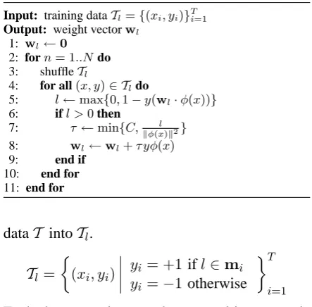
Algorithm 1 Passive-Aggressive algorithm for training a bi-nary classifier (PA-I).
Input: training dataTl={(xi, yi)}Ti=1
Output: weight vectorwl
1: wl←0
2: forn= 1..Ndo 3: shuffleTl
4: for all(x, y)∈ Tldo
5: l←max{0,1−y(wl·ϕ(x))}
6: ifl >0then
7: τ ←min{C,∥ϕ(xl)∥2}
8: wl←wl+τ yϕ(x)
9: end if 10: end for 11: end for
dataT intoTl.
Tl =
{
(xi, yi)
yi = +1 ifl∈mi
yi =−1 otherwise
}T
i=1
Each document is treated as a positive example if it has label l; otherwise it is a negative exam-ple. Since local classifiers are independent of each other, we can trivially parallelize training.
We employ the Passive-Aggressive algorithm for training (Crammer et al., 2006). Specifically we use PA-I. The pseudo-code is given in Algo-rithm 1. We set the aggressiveness parameterCas 1.0.
3.2 Tree Model
Unlike the flat model, the tree model exploits the label hierarchy. Each local classifier is now asso-ciated with an edgep → cof the label hierarchy and has a weight vectorwp→c. Ifwp→c·ϕ(x)>0,
it means thatxwould belong to descendant(s) of
c. Edge classifiers are independent of each other and can be trained in parallel.
We consider two ways of constructing training dataTp→c.
ALL — All training data are used as before.
Tp→c=
(xi, yi)|
yi= +1if∃l∈mi, l∈leaves(c)
yi=−1otherwise
T
i=1
Each document is treated as a positive example if it belongs to a leaf node ofc, and the rest is nega-tive examples (Punera and Ghosh, 2008).
SIB — Negative examples are restricted docu-ments that belong to the leaves ofc’s siblings.
Tp→c=
(x, y)|
y = +1if∃l∈m, l∈leaves(c)
y =−1if∃l∈m, l∈leaves(p) andl /∈leaves(c)
Algorithm 2 Top-down local search.
Input: documentx
Output: label setm
1: q←[ROOT], m← {}
2: whileqis not empty do
3: p←pop out the first item ofq, t← {}
4: for allcsuch thatcis a child ofpdo 5: t←t∪ {(c,wp→c·ϕ(x))}
6: end for
7: u← {(c, s)∈t|s >0}
8: ifuis empty then
9: u ← {(c, s)}such thatchas the highest scores amongp’s children
10: end if
11: for all(c, s)∈udo 12: ifcis a leaf node then 13: m←m∪ {c} 14: else
15: appendctoq 16: end if
17: end for 18: end while
This leads to a compact model because low-level edges, which are overwhelming in number, have much smaller training data than high-level edges. This is a preferred choice in previous studies (Liu et al., 2005; Wang et al., 2011; Sasaki and Weis-senbacher, 2012).
3.3 Top-down Local Search
In previous studies, the tree model is usually ac-companied with top-down local search for decod-ing (Montejo-R´aez and Ure˜na-L´opez, 2006; Wang et al., 2011; Sasaki and Weissenbacher, 2012).5 Algorithm 2 is a basic form of top-down local search. At each node, we select children to which edge classifiers return positive scores (Lines 4–7). However, if no children have positive scores, we select one child with the highest score (Lines 8– 10). We repeat this until we reach leaves. The decoding of the flat model can be seen as a special case of this search.
Top-down local search is greedy, hierarchical pruning. If a higher-level classifier drops a child node, we no longer consider its descendants as output candidates. This drastically reduces the number of local classifications in comparison with the flat model. At the same time, however, this is a source of errors. In fact, a chain of local decisions accumulates errors, which is known as error prop-agation (Bennett and Nguyen, 2009). If the de-cision by a higher-level classifier was wrong, the model has no way of recovering from the error.
5For other methods, Punera and Ghosh (2008)
post-process local classifier outputs by isotonic tree regression.
To alleviate this problem, various modifica-tions have been proposed, which we collectively call post-training adjustment. Sasaki and Weis-senbacher (2012) combined broader candidate generation with post-hoc pruning. They first gen-erated a larger number of candidates by setting a negative threshold (e.g., −0.2) instead of 0 in Line 7. Then they filtered out unlikely la-bels by setting another threshold on the sum of (sigmoid-transformed) local scores of each can-didate’s path. S-cut (Montejo-R´aez and Ure˜na-L´opez, 2006; Wang et al., 2011) adjusts the thresh-old for each classifier. R-cut selects top-r candi-dates either globally (Liu et al., 2005; Montejo-R´aez and Ure˜na-L´opez, 2006) or at each parent node (Wang et al., 2011). Wang et al. (2011) developed a meta-classifier which classified a root-to-leaf path using sigmoid-transformed local scores and some additional features. All these methods assume that the models themselves are inherently imperfect and must be supplemented by additional parameters which are tuned manually or by using development data.
4 Proposed Method
4.1 Global Model
We see hierarchical multi-label text classification as a structured prediction problem. We propose a global model that jointly predictsm, ortree(m).
score(x,m) =w·Φ(x,tree(m))
wcan be constructed simply by combining local edge classifiers.
w=wROOT→A⊕wROOT→B,· · · ,⊕wB→BB
Its corresponding feature function Φ(x,tree(m)) returns copies of ϕ(x), each of which corre-sponds to an edge of the label hierarchy. Thus score(x,m)can be reformulated as follows.
score(x,m) = ∑
p→c∈tree(m)
wp→c·ϕ(x)
Now we want to findmthat maximizes the global score,argmaxm score(x,m).
Algorithm 3MAXTREE(x, p)
Input: documentx, tree nodep
Output: label setm, scores 1: u← {}
2: for allcin the children ofpdo 3: ifcis a leaf then
4: u←u∪ {({c},wp→c·ϕ(x))}
5: else
6: (m′, s′)←MAXTREE(x, c)
7: u←u∪ {(m′, s′+wp→c·ϕ(x))}
8: end if 9: end for
10: r← {(m, s)∈u|s >0}
11: ifris empty then
12: r← {(m, s)}such that the item has the highest score samongu
13: end if
14: m←∪(m,s)∈rm
15: s←∑(m,s)∈rs 16: return (m, s)
4.2 Dynamic Programming
We show that an exact solution for the global model can be found by dynamic program-ming.6 The pseudo-code is given in Algorithm 3.
MAXTREE(x, p) recursively finds a subtree that maximizes the score rooted byp, and thus we in-voke MAXTREE(x,ROOT). Forp, each child c
is associated with (1) a set of labels that maxi-mizes the score of the subtree rooted bycand (2) its score (Lines 3–8). The score ofcis the sum of
c’s tree score and the score of the edgep → c. A leaf’s tree score is zero.
To maximizep’s tree score, we select all chil-dren that add positive scores to the parent (Line 10). If no children add positive scores, we select one child that gives the highest score (Lines 11– 13). Again, the flat model can be seen as a special case of this algorithm. The selected children cor-respond top’s label set and score (Lines 14–15).
A possible extension to this algorithm is to out-putN-best label sets. Since our algorithm is much easier than bottom-up parsing (McDonald et al., 2005), it would not be so difficult (Collins and Koo, 2005).
Dynamic programming resolves the search problem. We no longer require post-training ad-justment. It allows us to concentrate on improving the model itself.
6Bennett and Nguyen (2009) proposed a similar method,
but neither global model nor global training was considered. In their method, the scores of lower-level classifiers were in-corporated as meta-features of a higher-level classifier. All these classifiers were trained locally and required burden-some cross-validation techniques.
Algorithm 4 Modification to incorporate branching features. Replace Lines 10–15 of Algorithm 3.
10: r←usorted bysin descending order 11: r′← {}, s′←0, m′← {}
12: fork= 1..size ofrdo 13: (m, s)←r[k]
14: s′←s′+s, m′←m′∪m
15: r′←r′∪ {(m′, s′+wBF·ϕBF(p, k))}
16: end for
17: (m, s)←item inr′that has the highests
4.3 Inter-label Dependencies
Now we are ready to exploit inter-label depen-dencies. We introduce branching features, a sim-ple but powerful extension to the global model. They influence how many children a node selects. The corresponding function isϕBF(p, k), wherep
is a non-leaf node andkis the number of children to be selected forp. To avoid sparsity, we choose one ofR+ 1features (1,· · ·, Ror>R) for some pre-definedR. To be precise, we fire two features per non-leaf node: one is node-specific and the other is shared among non-leaf nodes. As a re-sult, we append at most(I+ 1)(R+ 1)features to the global weight vector, whereIis the number of non-leaf nodes.
All we have to do to incorporate branching fea-tures is to replace Lines 10–15 of Algorithm 3 with Algorithm 4. For givenk, we first need to selectk
children that maximize the sum of the scores. This can by done by sorting children by score and se-lect the first k children. We then add a score of branching featureswBF·ϕBF(p, k)(Line 15).
Fi-nally we chose a candidate with the highest score (Line 17).
4.4 Global Training
Up to this point, the global model is constructed by combining locally trained classifiers. Of course, we can directly train the global model. In fact we cannot incorporate branching features without global training.
Algorithm 5 shows a Passive-Aggressive algo-rithm for the structured output (Crammer et al., 2006). We can find an exact solution under the cur-rent weight vector by dynamic programming (Line 5).7 The costρ reflects the degree to which the model’s prediction was wrong. It is based on the
7If we want for some reason to stick to local search, we
Algorithm 5 Passive-Aggressive algorithm for global train-ing (PA-I, prediction-based updates).
Input: training dataT ={(xi,mi)}Ti=1
Output: weight vectorw
1: w←0
2: forn= 1..Ndo 3: shuffleT
4: for all(x,m)∈ T do
5: predictmˆ ←argmaxmscore(x,m)
6: ρ←1−2|m∩mˆ|/(|m|+|mˆ|)
7: ifρ >0then
8: l←score(x,m)ˆ −score(x,m) +√ρ 9: τ ←min{C, l
∥Φ(x,tree(m))−Φ(x,tree( ˆm))∥2}
10: w←w+τ(Φ(x,tree(m))−Φ(x,tree( ˆm)))
11: end if 12: end for 13: end for
example-based F measure, which will be reviewed in Section 5.3.
Note that what are called “global” in some pre-vious studies are in fact path-based methods (Qiu et al., 2009; Qiu et al., 2011; Wang et al., 2011; Sasaki and Weissenbacher, 2012). In contrast, we present tree-wide optimization.
4.5 Parallelization of Global Training
One problem with global training is speed. We can no longer train local classifiers in parallel because global training makes the model monolithic. Even worse, label set prediction is orders of magnitude slower than a binary classification. For these rea-sons, global training is extremely slow.
We resort to iterative parameter mixing (Mc-Donald et al., 2010). The basic idea is to split training data into small “shards” instead of sub-dividing the model. Algorithm 6 gives a pseudo-code, where S is the number of shards. We per-form training on each shard in parallel. At the end of each iteration, we average the models and use the resultant model as the initial value for the next iteration.
Iterative parameter mixing was originally pro-posed for Perceptron training. However, as Mc-Donald et al. (2010) noted, it is possible to pro-vide theoretical guarantees for distributed online Passive-Aggressive learning.
5 Experiments
5.1 Dataset
We used JSTPlus, a bibliographic database on sci-ence, technology and medicine built by Japan Sci-ence and Technology Agency (JST).8 Each
docu-8http://www.jst.go.jp/EN/menu3/01.html
Algorithm 6 Iterative parameter mixing for global training.
Input: training dataT ={(xi,mi)}Ti=1
Output: weight vectorw
1: splitT intoS1,· · · SS
2: w←0
3: forn= 1..Ndo 4: fors= 1..Sdo
5: ws←asynchronously call Algorithm 5 with some modifications:T is replaced withSs,wis
initial-ized withwinstead of0, andNis set as 1. 6: end for
7: join
8: w←S1∑Ss=1ws
9: end for
ment consisted of a title, an abstract, a list of au-thors, a journal name, a set of categories and many other fields. For experiments, we selected a set of documents that (1) were dated 2010 and (2) con-tained both Japanese title and abstract. As a result, we obtained 455,311 documents, which were split into 409,892 documents for training and 45,419 documents for evaluation.
The number of labels was 3,209, which amounts to 4,030 edges. All the leave nodes are located at the fifth level (the root not counted). Some edges skip intermediate levels (e.g., children of a second-level node are located at the fourth second-level). On aver-age 1.85 categories were assigned to a document, with a variance of 0.85. The maximum number of categories per document was 9.
For the feature representation of a document
ϕ(x), we employed two types of features.
1. Journal name (binary). One feature was fired per document.
2. Content words in the title and abstract (frequency-valued). Frequencies of the words in the title were multiplied by two.
To extract content words, we first applied the mor-phological analyzer JUMAN9 to each sentence to segment it into a word sequence. From each word sequence, we selected content words using the dependency parser KNP,10 which tagged content words at a pre-processing step. Each document contained 380 characters on average, which cor-responded to 120 content words according to JU-MAN and KNP.
9
http://nlp.ist.i.kyoto-u.ac.jp/EN/ index.php?JUMAN
10http://nlp.ist.i.kyoto-u.ac.jp/EN/
5.2 Models
In addition to the flat model (FLAT), the tree model with various configurations was compared. We performed local training of edge classifiers on ALL data and SIB data as explained in Sec-tion 3.2. We applied top-down local search (LS) and dynamic programming (DP) for decoding. We also performed global training (GT) with and without branching features (BF).
We performed 10 iterations for training local classifiers. For iterative parameter mixing de-scribed in Section 4.5, we evenly split the train-ing data into 10 shards and ran 10 iterations. For branching features introduced in Section 4.3, we setR = 3.
5.3 Evaluation Measures
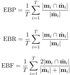
Various evaluation measures have been proposed to handle multiple labels. The first group of eval-uation measures we adopted is document-oriented measures often referred to as example-based mea-sures (Godbole and Sarawagi, 2004; Tsoumakas et al., 2010). The example-based precision (EBP), recall (EBR) and F measure (EBF) are defined as follows.
EBP = 1
T
T
∑
i=1
|mi∩mˆi|
|mˆi|
EBR = 1
T
T
∑
i=1
|mi∩mˆi|
|mi|
EBF = 1
T
T
∑
i=1
2|mi∩mˆi|
|mˆi|+|mi|
where T is the number of documents in the test data, mi is a set of correct labels of thei-th
doc-ument and mˆi is a set of labels predicted by the
model.
Another group of measures are called label-based (LB) and are label-based on the precision, re-call and F measure of each label (Tsoumakas et al., 2010). Multiple label scores are combined by performing macro-averaging (Ma) or micro-averaging (Mi), resulting in six measures.
Lastly we used hierarchical evaluation mea-sures to give some scores to “partially correct” labels (Kiritchenko, 2005). If we assume a tree instead of a more general directed acyclic graph, we can formulate the (micro-average) hierarchical
precision (hP) and hierarchical recall (hR) as fol-lows.
hP =
∑T
i=1∑|tree(mi)∩tree( ˆmi)|
T
i=1|tree( ˆmi)|
hR =
∑T
i=1|tree(mi)∩tree( ˆmi)|
∑T
i=1|tree(mi)|
The hierarchical F measure (hF) is the harmonic mean of hP and hR.
[image:6.595.118.241.422.553.2]5.4 Results
Table 1 shows the performance comparison of var-ious models. DP-GT-BF performed best in 5 mea-sures. Compared with FLAT, DP-GT-BF drasti-cally improved LBMiP and hP. Branching features consistently improved F measures. The tree model with local search was generally outperformed by the flat model. Compared with FLAT, DP-ALL and DP-GT, DP-GT-BF yielded statistically sig-nificant improvements withp <0.01.
DP-ALL outperformed LS-ALL for all but one measures. DP-SIB performed extremely poorly while DP-ALL was competitive with DP-GT-BF. This is in sharp contrast to the pair of LS-ALL and LS-SIB, which performed similarly. Dynamic programming forced DP-SIB’s local classifiers to classify what were completely new to them be-cause they had been trained only on small portions of data. The result was highly unpredictable.
As expected, dynamic programming was much slower than local search. In fact DP-GT-BF was more than 60 times slower than local search. Somewhat surprisingly, it took only 18% more time than FLAT. This may be explained by the fact that DP-GT-BF was 16% smaller in size than FLAT.
Although ALL was competitive with DP-GT and DP-DP-GT-BF, it is notable that global train-ing yielded much smaller models. Branchtrain-ing fea-tures brought further model size reduction along with almost consistent performance improvement. This result seems to support our hypothesis con-cerning the decision-making process of the human annotators. They do not select each label indepen-dently but consider the relative importance among competing labels.
5.5 Discussion
model iterations time (min) size EBP EBR EBF
FLAT 10 266 73M .4520 .4111 .3956
LS-ALL 10 5 115M .3927 .4064 .3713
LS-SIB 10 5 39M .4010 .4396 .3881
DP-ALL 10 329 115M .4790 .4336 .4247
DP-SIB 10 298 39M .0026 .6804 .0481
DP-GT 10 310 68M .5177 .4096 .4317
DP-GT-BF 10 315 62M .5172 .4121 .4347
[image:7.595.87.511.59.290.2]model LBMaP LBMaR LBMaF LBMiP LBMiR LBMiF hP hR hF FLAT .4260 .2549 .2578 .4155 .3727 .3930 .5343 .4746 .5027 LS-ALL .3288 .2764 .2415 .3622 .3716 .3668 .4988 .5060 .5024 LS-SIB .3291 .2989 .2515 .3415 .4066 .3712 .4750 .5359 .5036 DP-ALL .4576 .2760 .2799 .4542 .3933 .4216 .6020 .5163 .5559 DP-SIB .0267 .5214 .0406 .0184 .6649 .0358 .0031 .8104 .0600 DP-GT .4301 .2708 .2659 .5085 .3655 .4253 .6458 .4843 .5535 DP-GT-BF .4519 .2645 .2709 .5132 .3701 .4300 .6493 .4898 .5584
Table 1: Performance comparison of various models. Time is the one required to classify test data. Loading time was not counted. Size is defined as the number of elements in the weight vector whose absolute values are greater than10−7.
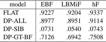
[image:7.595.318.521.355.466.2]model EBF LBMiF hF FLAT .9227 .9204 .9337 DP-ALL .8977 .8951 .9114 DP-SIB .0731 .0540 .0743 DP-GT-BF .7126 .6942 .7508
Table 2: Performance on the training data.
than DP-GT-BF although they were outperformed on the test data. It seems safe to conclude that local training caused overfitting.
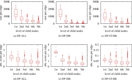
We further investigated the models by decom-posing them into edges. Figure 2 compares three models. The first three figures (a–c) report the number of non-trivial elements in each weight vector. Edges are grouped by the level of child nodes. Although DP-GT-BR was much smaller in total size than DP-ALL, the per-edge size distri-butions looked alike. The higher the level was, the larger number of non-trivial features each model required. Compared with DP-SIB, DP-GT-BR had compact local classifiers for the highest-level edges but the rest was generally larger. Intuitively, knowing its siblings is not enough for each local classifier, but it does not need to know all possible rivals.
The last three figures (d–f) report the averaged absolute scores of each edge that were calculated from the model output for the test data. By doing
"-" matrix
R 1st 2nd 3rd 4th
level of parent nodes 1
2 3 >3
# of children -0.2
-0.15 -0.1 -0.05
Figure 3: Heat map of the weight vector for branching features. R is the root level.
this, we would like to measure how edges of var-ious levels affect the model output. Higher-level edges tended to have larger impact. However, we can see that in DP-GT-BR, their impact was rel-atively small. In other words, lower-level edges played more important roles in DP-GT-BR than in other models.
[image:7.595.93.269.357.427.2]0 100K 200K 300K
1st 2nd 3rd 4th 5th
size per edge
level of child nodes
(a) DP-ALL.
0 100K 200K 300K
1st 2nd 3rd 4th 5th
size per edge
level of child nodes
(b) DP-SIB.
0 100K 200K 300K
1st 2nd 3rd 4th 5th
size per edge
level of child nodes
(c) DP-GT-BR.
0 1 2 3 4
1st 2nd 3rd 4th 5th
abs. score per edge
level of child nodes
(d) DP-ALL.
0 1 2 3 4
1st 2nd 3rd 4th 5th
abs. score per edge
level of child nodes
(e) DP-SIB.
0 0.05 0.1 0.15 0.2
1st 2nd 3rd 4th 5th
abs. score per edge
level of child nodes
[image:8.595.78.528.69.342.2](f) DP-GT-BR.
Figure 2: Comparison of model sizes and scores per edge. The definition of size is the same as that in Table 1.
hypothesis about the competitive nature of label candidates positioned proximally in the label hier-archy.
6 Conclusion
In this paper, we treated hierarchical multi-label text classification as a structured prediction prob-lem. Under this framework, we proposed (1) dynamic programming that finds an exact solu-tion, (2) global training and (3) branching features that capture inter-label dependencies. Branching features improve performance while reducing the model size. This result suggests that the selection of multiple labels by human annotators greatly de-pends on the relative importance among compet-ing labels.
Exploring features that capture other types of inter-label dependencies is a good research direc-tion. For example, “Others” labels probably be-have atypically in relation to their siblings. While we focus on the setting where only the leaf nodes represent valid labels, internal nodes are some-times used as valid labels. Such internal nodes of-ten block the selection of their descendants. Also, we would like to work on directed acyclic graphs and to improve scalability in the future.
Acknowledgments
We thank the Department of Databases for Infor-mation and Knowledge Infrastructure, Japan Sci-ence and Technology Agency for providing JST-Plus and helping us understand the database. This work was partly supported by JST CREST.
References
Paul N. Bennett and Nam Nguyen. 2009. Refined ex-perts: improving classification in large taxonomies. In Proceedings of the 32nd international ACM
SI-GIR conference on Research and development in in-formation retrieval, SIGIR ’09, pages 11–18.
Brent Berlin. 1992. Ethnobiological classification: principles of categorization of plants and animals in traditional societies. Princeton University Press.
Michael Collins and Terry Koo. 2005. Discriminative reranking for natural language parsing.
Computa-tional Linguistics, 31(1):25–70.
Michael Collins and Brian Roark. 2004. Incremen-tal parsing with the Perceptron algorithm. In
Pro-ceedings of the 42nd Meeting of the Association for Computational Linguistics (ACL’04), Main Volume,
pages 111–118.
passive-aggressive algorithms. Journal of Machine
Learning Research, 7:551–585.
Shantanu Godbole and Sunita Sarawagi. 2004. Dis-criminative methods for multi-labeled classifica-tion. In Honghua Dai, Ramakrishnan Srikant, and Chengqi Zhang, editors, Advances in
Knowl-edge Discovery and Data Mining, volume 3056 of Lecture Notes in Computer Science, pages 22–30.
Springer Berlin Heidelberg.
Liang Huang, Suphan Fayong, and Yang Guo. 2012. Structured Perceptron with inexact search. In
Pro-ceedings of the 2012 Conference of the North Amer-ican Chapter of the Association for Computational Linguistics: Human Language Technologies, pages
142–151.
Svetlana Kiritchenko. 2005. Hierarchical Text
Cat-egorization and Its Application to Bioinformatics.
Ph.D. thesis, University of Ottawa.
Yannis Labrou and Tim Finin. 1999. Yahoo! as an ontology: using Yahoo! categories to describe doc-uments. In Proceedings of the eighth international
conference on Information and knowledge manage-ment, CIKM ’99, pages 180–187.
Tie-Yan Liu, Yiming Yang, Hao Wan, Hua-Jun Zeng, Zheng Chen, and Wei-Ying Ma. 2005. Support vector machines classification with a very large-scale taxonomy. SIGKDD Explorations Newsletter, 7(1):36–43, June.
LSHTC3. 2012. ECML/PKDD-2012 Discovery
Chal-lenge Workshop on Large-Scale Hierarchical Text Classification.
Ryan McDonald, Koby Crammer, and Fernando Pereira. 2005. Online large-margin training of de-pendency parsers. In Proceedings of the 43rd
An-nual Meeting of the Association for Computational Linguistics (ACL’05), pages 91–98.
Ryan McDonald, Keith Hall, and Gideon Mann. 2010. Distributed training strategies for the structured Per-ceptron. In Human Language Technologies: The
2010 Annual Conference of the North American Chapter of the Association for Computational Lin-guistics, pages 456–464.
Arturo Montejo-R´aez and Luis Alfonso Ure˜na-L´opez. 2006. Selection strategies for multi-label text cate-gorization. In Advances in Natural Language
Pro-cessing, pages 585–592. Springer.
Kunal Punera and Joydeep Ghosh. 2008. Enhanced hierarchical classification via isotonic smoothing. In
Proceedings of the 17th international conference on World Wide Web, WWW ’08, pages 151–160.
Xipeng Qiu, Wenjun Gao, and Xuanjing Huang. 2009. Hierarchical multi-label text categorization with global margin maximization. In Proc. of the
ACL-IJCNLP Short, pages 165–168.
Xipeng Qiu, Xuanjing Huang, Zhao Liu, and Jinlong Zhou. 2011. Hierarchical text classification with latent concepts. In Proc. of ACL, pages 598–602.
Yutaka Sasaki and Davy Weissenbacher. 2012. TTI’S system for the LSHTC3 challenge. In
ECML/PKDD-2012 Discovery Challenge Workshop on Large-Scale Hierarchical Text Classification.
Grigorios Tsoumakas, Ioannis Katakis, and Ioannis Vlahavas. 2010. Mining multi-label data. In Oded Maimon and Lior Rokach, editors, Data Mining and
Knowledge Discovery Handbook, pages 667–685.
Springer.
Xiao-Lin Wang, Hai Zhao, and Bao-Liang Lu. 2011. Enhance top-down method with meta-classification for very large-scale hierarchical classification. In