R E S E A R C H
Open Access
Novel two-dimensional DOA estimation with
L-shaped array
Zhang Xiaofei
*, Li Jianfeng and Xu Lingyun
Abstract
Two-dimensional (2D) direction-of-arrival (DOA) estimation has played an important role in array signal processing. In this article, we address a problem of bind 2D-DOA estimation with L-shaped array. This article links the 2D-DOA estimation problem to the trilinear model. To exploit this link, we derive a trilinear decomposition-based 2D-DOA estimation algorithm in L-shaped array. Without spectral peak searching and pairing, the proposed algorithm employs well. Moreover, our algorithm has much better 2D-DOA estimation performance than the estimation of signal parameters via rotational invariance technique algorithms and propagator method. Simulation results illustrate validity of the algorithm.
Keywords:array antennas, direction-of-arrival estimation, L-shaped ar-ray
1. Introduction
Antenna arrays have been used in many fields, such as radar, sonar, communications, seismic data processing, and so on. The direction-of-arrival (DOA) estimation of signals impinging on an array of sensors is a fundamen-tal problem in array processing, and many DOA estima-tion methods have been proposed for its soluestima-tion [1-10]. Uniform linear arrays for estimation of wave arrival have extensively been studied. Compared with uniform linear array, L-shaped array can identify two-dimen-sional (2D) DOA. 2D-DOA estimation with L-shaped array has been received considerable attention in the field of array signal processing [5-13], and it contains estimation of signal parameters via rotational invariance techniques (ESPRIT) algorithms [5-7], multiple signal classification (MUSIC) algorithm [8], matrix pencil methods [9,10], propagator methods [11-13], and high-order cumulant method [14].
High-order cumulant method requires the signal sta-tistical properties, and it needs a heavy computation load. MUSIC algorithm is based on the noise subspace, and has a good DOA estimation performance. However, MUSIC requires spectral peak searching, which is putationally expensive. Propagator method has low com-plexity, but its 2D-DOA estimation performance is less
than ESPRIT algorithm. ESPRIT produces signal para-meter estimates directly in terms of (generalized) eigen-values, and the primary computational advantage of ESPRIT is that it eliminates the search procedure inher-ent. Authors of [5,6] used ESPRIT method for 2D-DOA estimation with L-shaped array, and Zhang et al. [7] proposed the improved ESPRIT algorithm for 2D-DOA estimation, which had better 2D-DOA estimation per-formance than that of [5,6]. The algorithms in [5-7] require an extra paring within 2D-DOA estimation. Par-ing usually fails to work in the condition of low signal-to-noise ratio (SNR) and the large number of sources.
This study links 2D-DOA estimation problem of L-shaped array to trilinear model, and derives a novel blind 2D-DOA algorithm whose performance is better DOA estimation than ESPRIT algorithms and propaga-tor method. Furthermore, our algorithm employs well without spectral peak searching and pairing. Bro et al. [15] proposed a 2D-DOA algorithm for uniform squares array using trilinear decomposition. There are some dif-ferences between this study and that of [15] in some aspects. First, Bro et al. [15] proposed a 2D-DOA algo-rithm for uniform squares array, while this study is to estimate 2D-DOA for L-shaped array. Second, the received signal of uniform squares array can be modeled directly with trilinear model, and then that of [15] pro-posed joint azimuth-elevation estimation using trilinear decomposition in uniform squares array. This article is * Correspondence: [email protected]
Department of Electronic Engineering, Nanjing University of Aeronautics & Astronautics, Nanjing 210016, China
to estimate 2D-DOA estimation in L-shaped array, and the received signal of L-shaped array cannot be modeled directly with trilinear model. We use the cross correla-tion of received signal for constructing the trilinear model.
The rest of the article is structured as follows. Section 2 develops a data model. Section 3 deals with algorith-mic issues. Section 4 presents simulation results, and Section 5 provides conclusions.
2. Data model
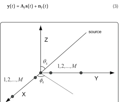
We consider an L-shaped array with 2M -1 sensors at different locations as shown in Figure 1. A uniform lin-ear array containingM elements is located iny-axis, and the other uniform linear array containingM elements is located inx-axis. We suppose that there are Ksources impinge on the L-shaped array with (θk,jk),k= 1,2,...,K, where θk,jk are the elevation and the azimuth angles of the kth source, respectively. The received signal ofM
elements inx-axis is
x(t) =Axs(t) +nx(t) (1)
wheres(t)∈CKis the source matrix,nx(t)∈CMis an M × 1 Gaussian white noise vector of zeros mean and covariance matrixs2IM, and Ax∈CM×K is
Ax=
⎡ ⎢ ⎢ ⎢ ⎣
1 1 · · · 1
e−jα1 e−jα2 · · · e−jαK ..
. ... . .. ...
e−j(M−1)α1e−j(M−1)α2· · · e−j(M−1)αK
⎤ ⎥ ⎥ ⎥
⎦ (2)
whereak= 2πdcosθksinjk/ l(k= 1, ...,K),dis the element spacing, and l is the wavelength. d ≤ l/2 is required in the array.
The received signal ofMelements iny-axis is denoted as
y(t) =Ays(t) +ny(t) (3)
whereny(t) is an M × 1 Gaussian white noise vector of zeros mean and covariance matrix s2IM, and Ay∈CM×Kis
Ay=
⎡ ⎢ ⎢ ⎢ ⎣
1 1 · · · 1
e−jβ1 e−jβ2 · · · e−jβK
..
. ... . .. ...
e−j(M−1)β1e−j(M−1)β2· · · e−j(M−1)βK ⎤ ⎥ ⎥ ⎥
⎦ (4)
where bk= 2πdsinθk sinjk / l, k = 1, ..., K. Ax and Ay are Vandermonde matrices. x(t)∈CM, y(t)∈CM, Ax∈CM×Kand Ay∈CM×Kare denoted as
x(t) =
x1(t)
xM =
x1
x2(t) (5)
y(t) =
y1(t)
yM =
y1
y2(t) (6)
Ax=
Ax1
axM =
ax1
Ax2 (7)
Ay=
Ay1 ayM =
ay1
Ay2 (8)
wherex1and xMare first and last rows ofx(t), respec-tively. y1 and yM are first and last rows of the y(t), respectively. ax1 and axMare first and last rows of the matrix Ax, respectively. ay1 and ayM are first and last rows of the matrixAy, respectively.
According to Equations 5-8, we construct the follow-ing matrices
C1=E{x1(t)y1(t)H}=Ax1RSAHy1+N1 (9)
C2=E{x2(t)y1(t)H}=Ax1xRSAHy1+N2 (10)
C3=E{x1(t)y2(t)H}=Ax1RSHyA H
y1+N3 (11)
C4=E{x2(t)y2(t)H}=Ax1xRSHyAHy1+N4 (12)
where x= diag(e−jα1,e−jα2,. . .,e−jαK),E{.} is the expectation,y= diag(e−jβ1,e−jβ2,. . .,e−jβK),RS=E{s(t)s (t)H} is the source correlation matrix. For independent sources,RSshould be a diagonal matrix with main diag-onal vector r= [r1 r2 ...rK]. N1, N2, and N4 are shown as follows.
N1=
⎡ ⎢ ⎢ ⎢ ⎣
σ20· · · 0 0 0· · · 0
..
. ... . .. ... 0 0· · · 0
⎤ ⎥ ⎥ ⎥
⎦∈RK×K
1 2
, ,...,M
1 2
, ,...,M
k
T
k
I
N2=N3=N4= ⎡ ⎢ ⎢ ⎢ ⎣
0 0· · · 0 0 0· · · 0
.. . ... . .. ... 0 0· · · 0
⎤ ⎥ ⎥ ⎥
⎦∈RK×K
We define the matrixΩas
= ⎡ ⎢ ⎢ ⎣ r1
r1e−jα1
r1ejβ1
r1e−j(α1−β1)
r2
r2e−jα2
r2ejβ2
r2e−j(α2−β2) · · · · · · · · · · · ·
rK rKe−jαK
rKejβK rKej(αK−βK)
⎤ ⎥ ⎥
⎦ (13)
Equations 9-12 can be denoted by
Cl=Ax1Dl()AHy1+Nl,l= 1, 2, ..., 4 (14)
where Dl(.) is to extract thelth row of its matrix and construct a diagonal matrix out of it. Now, the noiseless signal in (14) can be denoted as a trilinear model [16-20], which is shown as
xm,n,l=
K
k=1am,kbn,khl,k, m= 1,. . .,M−1, n= 1,. . .,M−1, l= 1,. . ., 4 (15)
wheream, kis the (m,k) element of the matrixAx1,hl, k stands for the (l,k) element of the matrix Ω, bn, k represents the (n,k) element of the matrix A∗y1. We hereby consider the signal in (15) as slicing the trilinear model along a direction, within which the symmetry characteristics allow other matrix system rearrange-ments
Ym=A∗y1Dm(Ax1) T
, m= 1,. . .,M−1 (16)
Zn=Dn(A∗y1)A T
x1 n= 1,. . .,M−1 (17)
3. Blind 2D DOA estimation
In this section, we utilize the trilinear decomposition for blind 2D-DOA estimation in L-shaped array, where the received signal has been reconstructed with trilinear model. We use trilinear decomposition for obtaining the direction matricesAˆx1andAˆy1, and then DOAs are esti-mated according to least square (LS) principle.
3.1 Trilinear decomposition
Since trilinear alternating LS (TALS) algorithm is a common data detection method for trilinear model [19], it can be discussed in detail as follows. According to (14), we construct the following matrix in this form
C= ⎡ ⎢ ⎢ ⎣ C1 C2 C3 C4 ⎤ ⎥ ⎥
⎦= [Ax1]AHy1+ ⎡ ⎢ ⎢ ⎣ N1 N2 N3 N4 ⎤ ⎥ ⎥ ⎦ (18)
where ⊙stands for Khatri-Rao product. LS fitting is given by
min
,Ax1,Ay1
C−[Ax1]AHy1
F (19)
LS update forAy1can be shown as
ˆ
AHy1 = [Ax1]+C (20)
Similarly, from the second way of slicing, we have Ym=A∗y1Dm(Ax1)
T, m= 1,. . .,M−1, which can be
rewritten as Y= ⎡ ⎢ ⎢ ⎢ ⎣ Y1 Y2 .. . YM−1
⎤ ⎥ ⎥ ⎥
⎦= [Ax1A∗y1]
T (21)
and the LS update forΩis
ˆ
T= [Ax1A∗y1]
+Y˜ (22)
whereY˜ is the noisy signal. Finally, from the third way
of slicing, we have
Zn=Dn(A∗y1)A T
x1, n= 1,. . .,M−1, which can be rewritten as Z= ⎡ ⎢ ⎢ ⎢ ⎣ Z1 Z2 .. . ZM−1
⎤ ⎥ ⎥ ⎥
⎦= [A∗y1]A
T
x1 (23)
and the LS update forAx1 is
ATx1= [A∗y1]+Z˜ (24)
whereZ˜ is the noisy signal.
According to (20), (22), and (24), the matricesAy1,Ω, and Ax1 are continually updated with conditional LSs, respectively, until convergence. TALS algorithm has sev-eral advantages: it is quite easy to implement, guarantee to converge, and comparatively simple to be expanded to the higher-order data. In this article, we use the com-plex-valued parallel factor analysis model (COMFAC) algorithm [17] for trilinear decomposition. COMFAC algorithm is essentially a fast implementation of TALS, and it can speed up the LS fitting.
For the blind 2D-DOA estimation algorithm that we have investigated, trilinear decomposition has been adopted for obtaining the estimated matrices, and then 2D-DOA estimation is correspondingly shown.
3.2 Identifiablity
Theorem 1 [19]: ConsideringCl=Ax1Dl()AHy1+Nl, l = 1,2, ...,4, where Ax1∈C(M−1)×K, Ay1∈C(M−1)×K, and
∈C4×K. Concerning that matrix, A
x1 and Ay1 have been provided with Vandermonde characteristics that the identifiability condition satisfies
k+ 2(M−1)≥2K+ 2 (25)
where kΩ is the kth rank [18] of the matrix Ω, the matrices Ay1, Ω, andAx1 are unique up to permutation and scaling of columns.
When the matrix∈C4×Kis fullkth rank, Equation
25 becomes
min(4,K) + 2(M−1)≥2K+ 2
IfK≥4, then min(4,K) = 4 and hence, the identifiabil-ity isK≤M. IfK≤ 4, then min(4,K) = Kand hence, the identifiability in practice becomesK≤2M- 4.
For the received noisy signal, we use trilinear decom-position for obtaining the estimated matricesAˆx1,ˆ, and
ˆ
Ay1, which are related toAy1,Ω, and Ax1via ˆ
Ax1=Ax11+V1 (26a)
ˆ
Ay1=Ay13+V3 (26b)
ˆ
=2+V2 (26c)
where∏is a permutation matrix,Δ1,Δ2,Δ3are diago-nal scaling matrices satisfying Δ1,Δ2, Δ3 =IK, V1, V2, and V3 are estimation error matrices. Within trilinear decomposition, permutation and scale ambiguities are inherent. Notably, the scale ambiguity can be resolved by means of normalization.
3.3 DOA estimation for L-shaped array
The direction matricesAˆx1and Aˆy1are obtained with tri-linear decomposition, and then angles are estimated.ax1 (θk,jk) is thekth column ofAx1, and it is
ax1(θk,φk) = [1,e−jαk,. . .,e−j(M−2)αk]T
and then the following vector is obtained by
gx=−angle(ax1(θk,φk)) = [0,αk,. . ., (M−2)αk]T(27)
where angle(.) is get the phase angles, for each ele-ment of complex array. Thereafter, LS principle is adopted for estimating sin jk cos θk. The estimated array steer vectoraˆx1(θk,φk)(thekth column of the
esti-mated matrix Aˆx1) is processed through normalization, which also resolves the scale ambiguity, and then nor-malized sequence is processed for attaininggˆxaccording to (27). LSs’fitting isPw=gˆx, where
P=
⎡ ⎢ ⎢ ⎢ ⎣
1 1 .. . 1
0 2πd/λ
.. . (M−2)2πd/λ
⎤ ⎥ ⎥ ⎥ ⎦,
w= [w0,wx]T, in whichwxis the estimated value of sin jkcosθk, andw0 is the other estimation parameter. The LS solution towis
ˆ w=
ˆ
w0 ˆ
wx = (P
TP)−1PTgˆ
x (28)
Similarly, ay1(θk,φk) = [1,e−jβk,. . .,e−j(M−2)βk]T is the kth column ofAy1, and then the corresponding vector is gy= -angle(ay1(θk, jk)) = [0,bk,...,(M-2)bk]T. We use Aˆy1 and LS principle to obtainwˆy, which is the estimation of sinjksinθk. The 2D-DOAs are estimated via
ˆ
φk= sin−1
ˆ
w2
x+wˆ2y
(29)
ˆ
θk= tan−1(wˆy/wˆx) (30)
Up to now, as deducted above, we have proposed the trilinear decomposition-based 2D-DOA estimation for L-shaped array in this section. The algorithmic steps in detail are shown as follows:
Step 1. We collect L snapshots to construct the matrices Ci, i= 1,2,...,4.
Step 2. According to the symmetry characteristics of trilinear model, we obtain Ym, m = 1,...,M - 1, andZnn = 1, ...,M-1.
Step 3. Initialize randomly for the matricesAy1,Ωand
Ax1.
Step 4. LS update for the source matrix Ay1 according to (20).
Step 5. LS update for the source matrix Ωaccording to (22).
Step 6. LS update for the channel matrix Ax1 accord-ing to (24).
Step 7. Repeat Steps 4-6 until convergence.
Step 8. Estimate 2D-DOA according to the estimated matrices and LSs principle.
It is noted that our algorithm can obtain automatically paired 2D-DOA estimation. In our algorithm, we employ trilinear decomposition for obtaining the esti-mated direction matrices Aˆx1=Ax11+V1,
ˆ
Ay1=Ay13+V3, which suffer from the same column permutation ambiguity, i.e., theith column ofAˆx1 corre-sponds to theith column of Aˆy1. So, our algorithm can estimate 2D-DOA estimation without extra pairing.
source matrix, followed by our algorithm to estimate coherent DOA. However, the spatial smoothing decreases the array aperture and the identifiable number of targets.
3.4 Complexity analysis and Cramer-Rao lower bounds (CRLB)
In contrast to ESPRIT algorithms in [6,7], our algorithm has a heavy computational load. For our algorithm, the complexity of each TALS iteration isO(3K3+ 12(M - 1) 2
K) [16], only a few iterations of this algorithm with COMFAC are usually required to achieve convergence. The total complexity of our algorithm isO{4L(M - 1)2+
n(3K3 + 12(M -1)2K)}, whereL is the number of snap-shots, andnis the number of iterations. The algorithm in [6] requires O(4L(M - 1)2 + 36(M - 1)3 + 2K3), and the ESPRIT algorithm in [7] needs O(4L(M - 1)2 + 80 (M -1)3+ 2K3).
We define the matrixA
A=
Ax
Ay2 ∈C
(2M−1)×K
which is also denoted byA= [a1a2...aK], whereaKis thekth column of the matrixA. According to [21], we derive the CRLB for angle estimation in L-shaped array,
CRLB = σ 2
2L
Re (DH⊥AD)⊕PT−1 (31)
where⊕stands for Hadamard product.
⊥
A=I2M−1−A(AHA)−1AH,P= 1 L
L l=1s(tl)s
H(t
l),D= [d1,d2,· · ·,dK,f1,f2,· · ·,fK],dk=∂ak/∂φk,fk=∂ak/∂θk.
4. Simulation results
We present Monte Carlo simulations that are to assess 2D-DOA estimation performance of the proposed algo-rithm. The number of Monte Carlo trials is 1000. There are two signals impinging on L-shaped array with (30°, 30°) and (40°, 40°), respectively. We consider the L-shaped array with2M- 1 sensors, and a half wavelength of the incoming signals is used for the spacing between the adjacent elements in each uniform linear array.L =
300 snapshots are used in the simulations.
Let RMSE = 1 K
K k=1
1 1000
1000
n=1 [(φˆk,n−φk) 2
+ (θˆk,n−θk) 2
],
whereθˆk,nis the estimate of the elevation angle θnof thenth Monte Carlo trial.φˆk,nis the estimation of the azimuth anglejkof thenth Monte Carlo trial.
We first investigate the convergence performance of our proposed algorithm in this simulation. The sum of squared residuals (SSR) in the trilinear fitting is defined as
SSR =
M−1
m=1
M−1
m=1 4
l=1
[x˜m,n,l−
K
k=1aˆm,kˆbn,khˆl,k] 2
where ˜xm,n,lis the noisy data. Define DSSR = SSRi -SSR0, where SSRiis the SSR of theith iteration, SSR0is the SSR in the convergence condition. Figure 2 shows the algorithmic convergence performance of COMFAC with 13-antenna-array and SNR = 15 dB. From Figure 2, we find that COMFAC needs few iterations to achieve convergence.
Figure 3 shows 2D-DOA estimation of the proposed algorithm at SNR = 15 dB, and Figure 4 shows 2D-DOA estimation of our algorithm at SNR = 24 dB. The L-shaped array with 13 antennas is used in Figures 3 and 4. From Figures 3 and 4, we find that our proposed algorithm employs well.
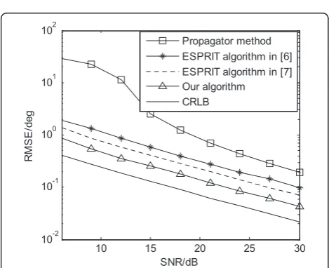
We compare our algorithm against ESPRIT algorithms [6,7], propagator method, and CRLB. Their DOA esti-mation performance comparison is shown in Figure 5, where the L-shaped array with 13 antennas is used. From Figure 5, we find that our algorithm has much better DOA estimation performance than ESPRIT algo-rithms and propagator method.
Figure 6 shows 2D-DOA estimation performance of our algorithm with different array configurations. It is seen from Figure 6 that 2D-DOA estimation perfor-mance of our algorithm is improved with the number of antennas increasing. When the number of antennas increases, our algorithm has higher received diversity.
5. Conclusion
This article links the L-shaped array 2D-DOA estima-tion problem to the trilinear model. To exploit this link,
1 2 3 4 5 6 7 8
10-10 10-5 100 105
iteration number
DS
S
R
COMFAC
we have proposed trilinear decomposition-based DOA estimation in L-shaped array. Without spectral peak searching and pairing, the proposed algorithm employs well. Furthermore, the proposed algorithm has much better 2D-DOA estimation performance than conven-tional ESPRIT algorithms and propagator method.
Notations
Bold symbols denote matrices or vectors. Operators (.)*, (.)T, (.)H, (.)-1, (.)+, and ||.||Fdenote the complex conju-gation, transpose, conjugate-transpose, inverse, pseudo-inverse, and Forbenius norm, respectively.IP denotes a P × P identity matrix. 1N×1is an N× 1 vector of ones. diag(v) stands for diagonal matrix whose diagonal is the vectorv. ⊙and ⊕stand for Khatri-Rao and Hadamard product, respectively.E{.} denotes statistical expectation.
Acknowledgements
This study was supported by the China NSF Grants (60801052), Aeronautical Science Foundation of China (2009ZC52036), Nanjing University of Aeronautics & Astronautics Research Funding (NS2010114, NP2011036) and the Graduate Innovative Base Open Funding of Nanjing University of Aeronautics & Astronautics.
Competing interests
The authors declare that they have no competing interests.
Received: 2 March 2011 Accepted: 30 August 2011 Published: 30 August 2011
References
1. X Zhang,Theory and application of array signal processing(National Defense Industry Press, Beijing, 2010)
2. X Zhang, D Xu, Improved coherent DOA estimation algorithm for uniform linear arrays. Int J Electron.96(2), 213–222 (2009). doi:10.1080/
00207210802526810
3. H Chen, B Huang, Y Wang, Direction-of-arrival estimation based on direct data domain (D3) method. J Syst Eng Electron.20(3), 512–518 (2009) 4. X Zhang, X Gao, D Xu, Multi-invariance ESPRIT-based blind DOA estimation
for MC-CDMA with an antenna array. IEEE Trans Veh Technol.58(8), 4686–4690 (2009)
25 30 35 40 45
28 30 32 34 36 38 40 42
elevation angle estimation/deg
az
im
ut
h ang
le es
tim
at
ion/
deg
Figure 32D-DOA estimation performance at SNR = 15 dB.
25 30 35 40 45
28 30 32 34 36 38 40 42
elevation angle estimation/deg
az
im
ut
h an
gl
e
es
tim
at
ion
/d
eg
Figure 42D-DOA estimation performance at SNR = 24 dB.
10 15 20 25 30
10-2 10-1 100 101 102
SNR/dB
R
M
SE/
de
g
Propagator method ESPRIT algorithm in [6] ESPRIT algorithm in [7] Our algorithm CRLB
Figure 5Angle estimation performance comparison.
10 15 20 25 30
10-2 10-1 100 101
SNR/dB
RM
S
E
/d
eg
array with 9 antennas array with 13 antennas array with 17 antennas
5. Y Dong, Y Wu, G Liao, A novel method for estimating 2-D DOA. J Xidian Univ.30(5), 369–373 (2003)
6. J Chen, S Wang, X Wei, New method for estimating two-dimensional direction of arrival based on L-shape array. J Jilin Univ (Eng Technol Edition) 36(4), 590–593 (2006)
7. X Zhang, X Gao, W Chen, Improved blind 2d-direction of arrival estimation with L-shaped array using shift invariance property. J Electromag Waves Appl.23(5), 593–606 (2009). doi:10.1163/156939309788019859
8. Y Hua, A pencil-MUSIC algorithm for finding two-dimensional angles and polarizations using crossed dipoles. IEEE Trans Antennas Propag.41(3), 370–376 (1993). doi:10.1109/8.233122
9. JE Fern’andez del R’ıo, MF C’atedra-P’erez, The matrix pencil method for two-dimensional direction of arrival estimation employing an L-shaped array. IEEE Trans Antennas Propag.45(11), 1693–1694 (1997). doi:10.1109/ 8.650082
10. P Krekel, E Deprettre, A two dimensional version of matrix pencil method to solve the DOA problem, inProceedings of European Conference on Circuit Theory and Design435–439 (1989)
11. N Tayem, HM Kwon, L-shape-2-D arrival angle estimation with propagator method. IEEE Trans Antennas Propag.53(5), 1622–1630 (2005)
12. P Li, B Yu, J Sun, A new method for two-dimensional array signal processing in unknown noise environments. Signal Process.47(3), 319–327 (1995). doi:10.1016/0165-1684(95)00118-2
13. Y Wu, G Liao, HC So, A fast algorithm for 2-D direction-of-arrival estimation. Signal Process.83(8), 1827–1831 (2003). doi:10.1016/S0165-1684(03)00118-X 14. B Tang, X Xiao, T Shi, A novel method for estimating spatial 2-D direction
of arrival. Acta Electonica Sinica27(3), 104–106 (1999)
15. R Bro, ND Sidiropoulos, GB Giannakis, Optimal joint azimuth-elevation and signal-array response estimation using parallel factor analysis, inProceedings of 32nd Asilomar Conference Signals, System, and Computer, 1594–1598 (1998)
16. SA Vorobyov, Y Rong, ND Sidiropoulos, Robust iterative fitting of multilinear models. IEEE Trans Signal Process.53(8), 2678–2689 (2005)
17. R Bro, ND Sidiropoulos, GB Giannakis, A fast least squares algorithm for separating trilinear mixtures, inProceedings of International Workshop ICA and BSS, 289–294, (1999)
18. ND Sidiropoulos, GB Giannakis, R Bro, Blind PARAFAC receivers for DS-CDMA systems. IEEE Trans Signal Process.48(3), 810–823 (2000). doi:10.1109/78.824675
19. ND Sidiropoulos, X Liu, Identifiability results for blind beamforming in incoherent multipath with small delay spread. IEEE Trans Signal Process. 49(1), 228–236 (2001). doi:10.1109/78.890366
20. X Zhang, G Feng, J Yu, Angle-frequency estimation using trilinear decomposition of the oversampled output. Wireless Pers Commun.51, 365–373 (2009). doi:10.1007/s11277-008-9652-5
21. P Stoica, A Nehorai, Performance study of conditional and unconditional direction-of-arrival estimation. IEEE Trans Signal Process.38, 1783–1795 (1990). doi:10.1109/29.60109
doi:10.1186/1687-6180-2011-50
Cite this article as:Xiaofeiet al.:Novel two-dimensional DOA estimation with L-shaped array.EURASIP Journal on Advances in Signal Processing 20112011:50.
Submit your manuscript to a
journal and benefi t from:
7Convenient online submission
7Rigorous peer review
7Immediate publication on acceptance
7Open access: articles freely available online
7High visibility within the fi eld
7Retaining the copyright to your article