Onset Detection in Surface Electromyographic Signals:
A SystematicComparison of Methods
Gerhard Staude
Institut für Mathematik und Datenverarbeitung, Universität der Bundeswehr München, Germany Email: [email protected]
Claus Flachenecker
Institut für Mathematik und Datenverarbeitung, Universität der Bundeswehr München, Germany Email: claus.fl[email protected]
Martin Daumer
Institut für Medizinische Statistik und Epidemiologie, Technische Universität München, Germany Email: [email protected]
Werner Wolf
Institut für Mathematik und Datenverarbeitung, Universität der Bundeswehr München, Germany Email: [email protected]
Received 26 July 2000 and in revised form 13 May 2001
Various methods to determine the onset of the electromyographic activity which occurs in response to a stimulus have been discussed in the literature over the last decade. Due to the stochastic characteristic of the surface electromyogram (SEMG), onset detection is a challenging task, especially in weak SEMG responses. The performance of the onset detection methods were tested, mostly by comparing their automated onset estimations to the manually determined onsets found by well-trained SEMG examiners. But a systematic comparison between methods, which reveals the benefits and the drawbacks of each method compared to the other ones and shows the specific dependence of the detection accuracy on signal parameters, is still lacking. In this paper, several classical threshold-based approaches as well as some statistically optimized algorithms were tested on large samples of simulated SEMG data with well-known signal parameters. Rating between methods is performed by comparing their performance to that of a statistically optimal maximum likelihood estimator which serves as reference method. In addition, performance was evaluated on real SEMG data obtained in a reaction time experiment. Results indicate that detection behavior strongly depends on SEMG parameters, such as onset rise time, signal-to-noise ratio or background activity level. It is shown that some of the threshold-based signal-power-estimation procedures are very sensitive to signal parameters, whereas statistically optimized algorithms are generally more robust.
Keywords and phrases:EMG, electromyography, onset detection method, performance, comparison.
1. INTRODUCTION
Analysis of electromyographic signals recorded from the skin over the muscles by surface electrodes (SEMG) represents an important tool in a variety of applications like neurological diagnosis, neuromuscular and psychomotor research, sports medicine, prosthetics, or rehabilitation. Processing of SEMG (and other biosignals like EEG, ENG, ECG, etc.) can be con-sidered a special field of applied signal processing, with the main focus on an appropriate application of theoretical con-cepts to extract specific information from small and often noisy biosignals.
times are unknown in real SEMG recordings, a rating by an objective error measure is not possible. Therefore, the auto-matically determined onsets are usually compared to results obtained by visual inspection of the data by some well-trained SEMG examiner. But a profound performance test should be based upon a relevant statistical analysis which requires a large amount of SEMG data with properly preset signal pa-rameters. This analysis is difficult or even impossible with real data due to the poor parameter reproducibility of successive SEMG recordings, and due to inter- and intra-rater variability introduced by the manually determined reference onset esti-mates. To overcome this problem, simulated SEMG data were used in this study for assessing the sensitivity of various detec-tion methods to changes in signal parameters. Also, the struc-ture of the various existing SEMG onset detection methods was analyzed revealing several common components which are identical in a logical way, but are formulated individually by different authors. As basis for comparison, some funda-mental algorithmic principles formulated in [12] were used to express each method by these terms.
Detection algorithms introduced earlier by Hodges and Bui [13], Bonato et al. [14], Lidierth [15], Abbink et al. [2], and two new implementations of the model-based detector proposed by Staude et al. [12] are included in this study. The algorithmic layout of the methods is compared, and the de-pendence of onset detection accuracy on signal parameters is demonstrated. The use of a statistically optimal estimator as a reference for the upper performance limit allows an absolute performance ranking of each method. In addition, the meth-ods were tested on real SEMG data obtained in a reaction time situation.
2. ONSET DETECTION ALGORITHMS 2.1. General scheme of onset detection
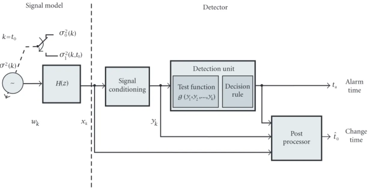
As suggested in [12], the comparison of algorithmic struc-tures is conducted by using the SEMG signal model and gen-eral scheme of event (onset) detection shown in Figure 1. The digitized SEMG signal may be represented by a real-valued se-quence(xk)k≥1, wherexkdenotes the signal amplitude at a
particular discrete time instantk; thus a single SEMG record (xk)k≥1 represents a sample observation of a discrete
ran-dom process (a zero mean discrete white Gaussian noise pro-cess)(Wk)k≥1exciting a linear system with transfer function
H(z).(Wk)k≥1reflects the discharge timing and recruitment
of the elementary signal sources (i.e., the motor units) in-volved;H(z)describes the shape of the discharges (i.e., the action potentials) as well as the specific bioelectrical transfer function between generator and recording site. Measurement noise is neglected.H(z)is modeled by an all-pole represen-tation (autoregressive (AR) filter) of orderp
H(z)=1+a 1
1z−1+a2z−2+ · · · +apz−p, (1)
wherea1, a2, . . . , ap are the AR coefficients and zdenotes
the complex frequency of thez-transform. The time domain representation of this signal model is
xk= − p
i=1
aixk−i+wk. (2)
As a particular feature of the signal model, the varianceσ2(k)
of the white noise excitation depends on the current state of the muscle activity which is modulated by descending com-mands from supraspinal levels as well as by feedback from peripheral receptors [16]. Within this framework, the indica-tion for the response onset to be detected is an abrupt change in the variance profileσ2(k), that is, it changes abruptly from
a patternσ2
0(k)to a new patternσ12(k, t0)≠σ02(k)at time
instantt0.
Computerized onset detection requires to determine the unknown change timet0 as accurate as possible. Most
detection algorithms consist of up to three basic processing stages (see Figure 1):
• signal conditioning, • detection unit, • post-processor.
In an initial step, the observed SEMG signal passes through a signal conditioning unit in order to enhance the spectral content of the measured signal carrying information about the onset of muscle activation. Frequently, a lowpass filter is applied to reduce high frequency noise. More sophisticatedly, an adaptive whitening filter can be used which eliminates the spectral color that was introduced by the bioelectrical channelH(z)but which is absolutely irrelevant for detection of changes in the excitation signal. The observed SEMG signal (xk)k≥1is processed by a filter with transfer function
Hw(z)=1+b1z−1+b2z−2+ · · · +bqz−q (3)
with the filter orderqand the filter coefficientsbituned to the
parameters of the shaping filterH(z). Obviously, forq=p andbi=ai, the whitening filter represents the ideal inverse
filterHw(z)=H−1(z)with respect to the transfer function H(z). Therefore, with the parameters ofH(z)exactly known, the excitation(wk)k≥1can completely be reconstructed.
Usu-ally, these parameters are unknown but can be estimated from the measured signal by some least-squares technique, for ex-ample [17].
In the next processing stage, a test function g(y1,
y2, . . . , yk)is computed from the (pre-conditioned) signal (yk)k≥1 which serves as an indicator for the response
on-set. The test function uses some or even all of the past samples to create an intermediate signal which is moni-tored by the decision rule in order to determine whether a change in the muscle activation pattern has occurred (alarm timeta). Some onset detection methods directly use
ta as an estimate ˆt0 for the SEMG onset time t0. Some
other methods use ta as a pure indicator for the
exis-tence of an onset and estimateˆt0through additional
post-processing.
The decision rules of all methods will be written in stopping rule notation,
y
kH
g , ,...
Alarm time
Change time Signal
conditioning
Detection unit
Post processor Test function Decision
rule ~
Signal model Detector
ˆ0
xk
(z)
(k)
0)
(k,t
(k)
a
yk wk
k=t0
2 1 2 0
2
1y2 ,yk
t t
) y ( σ
σ
σ
Figure1: Scheme of event detection in surface electromyographic signal (SEMG). The digitized SEMGxkis modeled by a white Gaussian
noise signal with dynamic varianceσ2(k)exciting a linear system with transfer functionH(z). Att0, the signal variance changes from resting activityσ2
0(k)toσ12(k, t0)of the active state. Most detectors employ up to three processing stages (signal conditioning, detection unit, and post-processor) in order to detect an event (alarm timeta) and to determine an estimate for the unknown change timet0.
wherehis an appropriate threshold. Each time a new data pointykis available, the current valuegkof the test function
is computed from the samplesy1, y2, . . . , ykand compared
to the thresholdh. As long asgk< h, this procedure is
re-peated sample by sample. At the first time instantta, when
gk≥h, the procedure is stopped, and an event alarm is given.
Estimation of the exact change time t0 by the
post-processor usually starts after event alarm was given atta, and
the estimateˆt0 of the unknown t0 is computed from the
samplesy1, y2, . . . , yta+∆. Some methods employ a separate signal conditioning unit which computes the input sequence for the post-processor from the raw SEMGx1, x2, . . . , xta+∆. Most algorithms require an additional amount∆of samples after the alarm time, thusta+∆represents the earliest time
instant when the final onset estimateˆt0is available. The
(op-tional) change time estimation procedure is written as
ˆ
t0=fy1, y2, . . . , yta+∆
, (5)
wheref is an arbitrary function that computes the change time fromy1, y2, . . . , yta+∆.
In the following two sections, commonly used detection methods are described within the framework of this basic computational structure shown in Figure 1. The summary of this analysis is presented in Table 1, together with the param-eter values chosen for their performance evaluation.
2.2. Selected threshold-based onset detection methods
Hodges and Bui
The detection algorithm proposed by Hodges and Bui [13] is a representative for a large class of detection methods, known
as finite moving average (FMA) algorithms (cf. [5, 8, 18, 19]). All these methods employ a fixed-size sliding test window, and the output at time k is computed as the weighted sum of theW signal samplesyk−W+1, yk−W+2, . . . , yk
con-tained within the window. Within the framework of Figure 1, theHodgesmethod first conducts some signal conditioning; SEMG data samples are rectified and subsequently lowpass filtered. From the pre-processed signal(yk)k≥1, the test
func-tiong(y1, y2, . . . , yk)at timekis computed as the mean of yk−W+1, yk−W+2, . . . , yk, and muscle activity onset is
identi-fied at the instant when the test function exceeds the baseline activity level by a specified multiplehof standard deviations. The baseline activity is adaptively determined by averaging the initialMsamples of(yk)k≥1. The algorithm can be
sum-marized by the following decision rule:
ta=mink≥W:gk≥h,
gk=σˆ1 0
˜
yk−µˆ0,
˜
yk=W1 k
i=k−W+1
yk,
ˆ
t0=ta−W+1,
(6)
whereyk denotes the rectified and lowpass filtered SEMG
signal, andµˆ0andσˆ0are the mean and standard deviation
of theM initial samples of (yk)k≥1, respectively. After the
stopping rule signaled an alarm, the first index of the sliding window is used as an estimate for the onset timet0, which is
Table1: Characteristic properties of all examined onset detection methods.
H
odges
B
onato
L
idier
th
A
bbink
A
GLRste
p
A
GLRr
amp
EstOpt
Signal conditioning
Pre-whitening × × × ×
Data sample rectification × × ×
Data sample squaring × × × ×
Lowpass filtering × ×
Test function/decision rule
Moving average + simple threshold × × ×
χ2test variable + double threshold ×
Likelihood ratio test × × ×
Post-processor/onset time estimation
Any threshold crossing ×
Threshold&duration-based selection of alarm time × ×
Search for maximum in (additional) test function × × × ×
Bonato et al.
The signal conditioning stage of theBonatomethod [14] con-sists of an adaptive whitening filter, with the filter parameters estimated from the current SEMG data. The test function is determined by two successive samples of(yk)k≥1
accord-ing to
gk= 1 ˆ
σ2 0
y2 k−1+yk2
, (7)
whereσˆ0is the standard deviation of theMinitial samples of
(yk)k≥1. Note thatgkis evaluated only for odd values ofk.
The decision rule is
ta=mink=1,3,5, . . .:gk≥h (8)
and the post-processor checks the resulting alarms for their relevance. It accepts the onset decision only, if both following rules apply:
• at leastnout ofmsuccessive samples must exceed the threshold in order to indicate the current muscle state to be an active state,
• such an active state must last for at leastT1samples.
If this check holds true, the earliest beginning of this active state epoch is taken as an estimate for the onset timet0.
As an important property, the method assumes that the pre-whitened SEMG (yk)k≥1 before the response onset is
represented by a sequence of statistically independent zero mean Gaussian random variables with equal variance. Thus, withσˆ02estimated from the measured sequence, the statistical
properties of the test functiongkcan be explicitly specified,
which facilitates a more sophisticated setting of the parame-tersh,n,m, andT1. Further, the use of a double-threshold
scheme in the post-processor provides a higher degree of freedom for selecting detection parameters. However, due to the implicit maximum operation of the “nout of m” cri-terion the accuracy with which the response onset can be
determined is limited by the sizemof the test window. More-over, the down-sampling operation reduces time resolution which may also lead to a less accurate onset estimation. Bon-atowas implemented with the parametersh=7.74,n=1, m=5,T1=50, andM=200.
Lidierth
Lidierth [15] proposed a full-wave rectification of the raw SEMG as signal conditioning only. The test function and de-cision rule of theLidierthdetection unit are identical to the Hodgesapproach, but increased performance is achieved by the extended post-processing rules:
• SEMG onset detection is accepted, if the test function exceeds the thresholdhto the active level for at least T1samples, and
• during T1, the test function may repeatedly fall
be-low the threshold, but each time not longer than T2samples.
Note that these post-processing rules represent a specific case of the post-processor suggested byBonato; with the param-eters of the Bonato“n out of m” criterion set to n = 1
andm = T2, both post-processing rules are identical, thus
Lidierthis a composite of BonatoandHodges.Lidierthwas implemented with parametersT1=90,T2=15,h=3, and
M=200.
Abbink et al.
Again, the “new” method copies the signal conditioning and detection unit from already known methods, and adds some specific fine tuning by extending the post-processor function: Abbink [2] uses the Hodges signal conditioning and detection unit approach, only changing the cutoff frequency to 3 Hz and the window length Wto 1.
The post-processor stage ofAbbinkuses a less smooth ver-sion(y
but-terworth lowpass with 30 Hz cutoff frequency to the rectified SEMG (i.e., the post-processor does his own signal condi-tioning). Looking backwards fromta, the following rules are
applied:
wherenlow(j)denotes the number of normalized amplitudes
smaller than the thresholdh2in theNsamples directly
pre-ceding the onset time candidatej, andnhigh(j)is the number
of amplitudes larger thanh2in theNsamples directly
follow-ingj. Meanµˆ0and standard deviationσˆ0are estimated from
the initialMsamples of(y
k)k≥1, respectively. The following
parameters were used for the simulations:h = 3,h2 = 3,
N=200, andM=200.
2.3. Detectors based upon statistically optimal decision
If the signal generating process is (partially) known, detectors based on statistically optimal decision rules can be used. In this section, three algorithms are presented which are derived from the model-based detection concept of [12]. In order to determine an estimate oft0, these methods evaluate the
statistical properties of the measured SEMG signal before and after a possible change in model parameters. Only basic processing steps are described here (see [12] for details). The specific implementations of the decision rules for the SEMG signal model (see Figure 1 left) are given in the appendix.
For signal conditioning, all 3 methods employ an adap-tive whitening filter for the reduction of irrelevant informa-tion. Assuming optimal performance of the filter, the (re-constructed) excitation signal(yk)k≥1=(wk)k≥1represents
a single realization of a statistically independent Gaussian random process(Yk)k≥1. The statistical properties of an
in-dividual random variable Yk can be fully described by its
probability density function (PDF)
pσ(yk)= 1
2πσ2(k)e−y
2
k/2σ2(k), (10)
which depends upon the (deterministic) variance profile σ2(k). The model-based decision rules for this problem
depend on the a priori knowledge about the variance pro-filesσ2
0(k)andσ12(k, t0)before and after the change to be
detected.
Optimal estimator (EstOpt) If the variance profilesσ2
0(k)andσ12(k, t0)are exactly known
(except the onset timet0), a statistically optimal decision rule
can be designed according to
ta=mink≥1 :gk≥h,
This detector referred to asEstOptalgorithm computes the maximum likelihood (ML) estimateˆt0of the unknown onset
timet0provided that all remaining parameters of the signal
model are exactly known. TheEstOptdecision rule is suited for arbitrary but known dynamic variance profilesσ2
0(k)and
σ12(k, j), thus it shows optimal performance among all
pos-sible algorithms for sequential detection in this application. Therefore, theEstOptdetector may serve as a reference for performance rating. (Essentially, the test compares the log-likelihood ratio
between the two distributions before and after a possible change at timejwith a thresholdh. Since the exact change timet0is unknown, it is replaced by its ML estimate, that is, a
maximum operator selects the largest value of the test func-tion with respect to all possible change times1≤j≤k. Each time a new data pointykis available, a test window with the
upper boundkfixed at the current observation and with its lower boundjcomprises all the observationsyj, yj+1, . . . , yk
after the hypothetical change timej. For each candidatej, the log-likelihood ratioSjk is computed from the observations
within the test window. If the maximum ofSk
jwith respect to
all hypothetical change times1≤j≤kexceeds the thresh-oldh, data acquisition stops and event alarm is given (alarm timeta). The timejat which the maximum value is obtained
serves as the maximum likelihood estimateˆt0of the unknown
change timet0.)
Approximated generalized likelihood-ratio detectors (AGLRstep, AGLRramp)
If the variance profilesσ2
0(k)andσ12(k, j)are not known like
inEstOpt, they can be replaced by estimates. For this condi-tion, the approximated generalized likelihood ratio (AGLR) detector [20] is an appropriate tool to formulate the stopping rule. First, the variance profiles are assumed to depend upon several unknown parameters, that is,
σ2
The unknown parameter vectorθ0, true up tot0, is estimated
ˆ
which is kept fixed throughout the remaining detection pro-cedure. Next, a sliding window of fixed sizeW is continu-ously shifted along the data sequence. For each locationkof the window, the ML estimateθˆ1of the unknown parameter
vectorθ1after change is determined from theWdata points
covered by the window, and the corresponding log-likelihood ratioSˆk
k−W+1is computed and compared with a thresholdh.
Finally, after a change has been indicated, the exact change time is estimated by an ML procedure from all possible can-didatesj≤ta. The AGLR decision rule can be summarized as
ta=mink≥W:gk≥h,
where∆is an appropriate dead zone which ensures that a minimum number of observations is available for parameter estimation. Note that the maximization with respect toθ1has
to be repeatedly performed for each combination(j, k)to be tested. Therefore, the computational effort is dominated by the number of operations required for computingθˆ1.
In this paper, two implementations of the AGLR decision rule are used which differ in the complexity ofσ2
1(k, j). The
AGLRstepalgorithm assumes a step-like variance profile with constant but different variances before and after change. This allows for a very efficient implementation of the method but completely disregards the available information about the dy-namic profile of the change itself. TheAGLRrampalgorithm explicitly takes this information into account by assuming a “ramp and hold” change profile. The unknown parametersθ1
of the transition are estimated from the actual observations. Thus, comparison of theAGLRstepandAGLRrampmethods shows the advantage of using available information about the change dynamics in the detection process. Their exact im-plementations for the present signal model are given in the appendix.
3. EVALUATION OF DETECTION PERFORMANCE ON SIMULATED SEMG RECORDINGS
3.1. Signal generation
All methods were tested for robustness and efficiency on a set of simulated SEMG traces which were generated by us-ing the signal model shown in Figure 1(left). The coefficients of the shaping filter were determined from a representative set of real SEMG data from a previous study [21] using
standard techniques of least squares parameter estimation [17]. Model order was set top=8. A total number of 16000 segments, each consisting of 1000 data points (i.e., 1000 ms record length) were generated. Figure 2 depicts the principle and definitions. The response to be detected was modeled by a rapid change in the varianceσ2(k)from a pattern
σ2
0(k)=σnoise2 (16)
to a new pattern
σ2
1k, t0=σnoise2 +σsignal2 uk, t0, (17)
wheret0 denotes the onset of the voluntary muscle
activa-tion,u(k, t0)describes the dynamic profile of the change,
andσnoise2 andσsignal2 are appropriate constants. The resting
activityσ2
noise0results from spontaneous firing of motor
units which occurs even if the muscle is not voluntarily acti-vated. (Note that the usage of the term “noise” is technically but not biologically motivated.)σsignal2 denotes the
magni-tude of the activation pattern. The dynamic change profile was approximated by a unit ramp and hold transition
uk, t0=
whereτ denotes the duration of the ramp. This finite slope of the change profile reflects the limited dynamics within the neuromuscular system [16], andτ was varied as it can be observed in real data. The onsett0of voluntary muscle
acti-vation was randomly varied between 400 ms and 600 ms, rel-ative to the beginning of the trace. Change magnitudeσ2
signal
was always set to 1 while background activityσnoise2 was varied
to create variable signal-to-noise ratios (SNR)
SNR=10·log10σ
Several sets of simulated SEMG traces, each consisting of 4000 trials, were used for testing the onset detection algorithms. The assessment of the onset detection accuracy was made for the following range of parameters (referenced asMixed Trials):
• ramp durationτuniformly distributed between 5 ms and 30 ms,
• signal-to-noise ratio SNR uniformly distributed be-tween 6 dB and 12 dB.
In particular, dependence on SNR and ramp duration were studied. Sensitivity to SNR was investigated with theMixed SNR Trialsdata set:
• fixed ramp durationτof 20 samples,
+
ramp duration signal
0 2
noise
2
noise 2
t
k
2( )k
τ σ
σ
σ σ
(a) Power envelope of modeled SEMG signals. After a period of background activity the SEMG power linearly rises to the active state withinτ. Parameters were systematically varied during simulation.
0 200 400 600 800 1000
0 1 2 3
0 ( )
x
k
k
t σ
−1
−2
−3
ms ( )
(b) Sample trace of simulated SEMG.
Figure2: Simulated SEMG.
• fixed ramp durationτof 20 samples, • fixed SNR of either 3 dB or 6 dB.
Sensitivity to ramp duration was investigated with theMixed Ramp Trialsdata set:
• ramp durationτuniformly distributed between 5 ms and 30 ms,
• fixed SNR of 10 dB.
All simulations were performed using MATLAB* (version 5.3, The MathWorks, Natick, MA) on an IBM-compatible PC.
3.2. Results of onset detection analysis
The aim of this paper is to objectively compare the perfor-mance of commonly used onset detection methods. It should be considered that several factors could influence detection performance:
• algorithmic delay of onset detection,
• percentage of missed responses and false alarm rate, • detection error bias, that is, average deviation between
estimated and true onset,
• reproducibility for signals with the same parameters,
• sensitivity of all attributes to SNR and onset ramp du-ration.
The first two factors refer to the detection power of the al-gorithm, that is, the ability of a method to signal an event as early as possible (small delay of alarm time ta)
com-bined with a false alarm rate as low as possible. Actually, due to the relatively high SNR, the majority of the simulated SEMG responses could be detected within a reasonable time range around the real onset, and the detection probability of all algorithms was nearly100%. We, therefore, focus on the remaining 3 factors which are related to the accuracy of the estimated change timest0.
Measures of detection performance
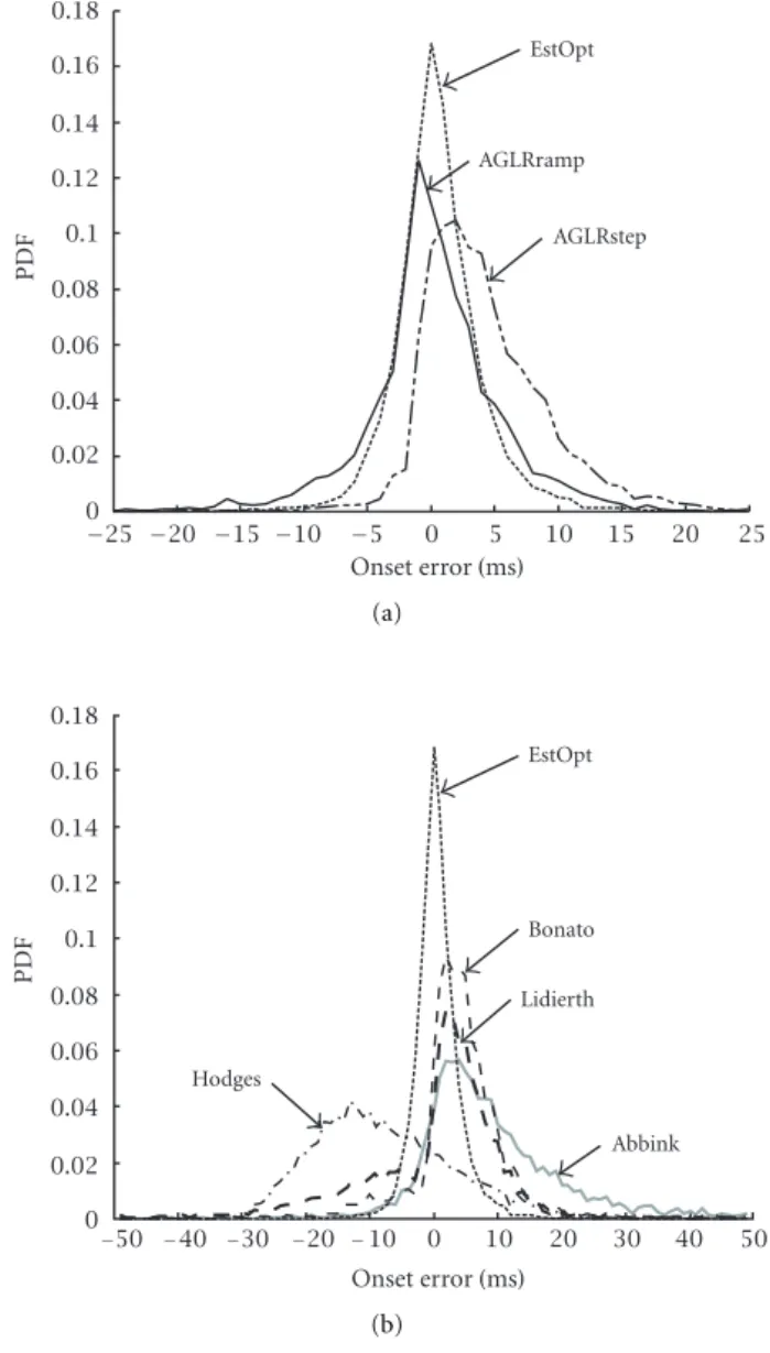
Figure 3 shows the probability density functions (PDFs) of the onset errorε = ˆt0−t0 for all methods (Mixed Trials).
EstOpt
−25 −20 −15 −10 −5 0 5 10 15 20 25 0
0.02 0.04 0.06 0.08 0.1 0.12 0.14 0.16 0.18
AGLRstep AGLRramp
Onset error (ms)
(a)
0 10 20 30 40
0 0.02 0.04 0.06 0.08 0.1 0.12 0.14 0.16 0.18
Onset error (ms) Bonato EstOpt
Abbink Lidierth
Hodges
50
− − − −
−50 40 30 20 10
(b)
Figure3: Probability density functions (PDFs) of onset estimation errors for theMixed Trialsdata set (SNR 6–12 dB, ramp duration 5–30 ms). Note the different abscissa scaling in (a) and (b).
AGLRrampmethod is still centered near the origin, the PDF ofAGLRstepis shifted towards higher onset errors. In the per-formance ranking,BonatoandLidierthfollow with reasonable results. Finally,Abbinkshows worse results because the PDF spreads to larger onset error values, andHodgesranks low-est because of a wide-spread distribution with additionally strong (negative) bias.
Table 2 depicts mean and standard deviation of onset estimation errors and the percentage of detected onsets with an absolute error less than 100 ms for each method. The 100 ms limit was chosen because it comprises at least 99%
of all onset estimates computed from theMixed SEMG Trials. Note that, due to the very thin tail of the PDF, variations in the limit will result in only minor variations of the result-ing probability of detected onset. Analysis of the mean er-rors in Table 2 shows that theAGLRrampalgorithm provides
Table2: Statistics for onset estimates based on SEMG data set “Mixed Trials.”
Method Detectedonsets Meanerror ErrorSTD
EstOpt 100.0% 0.6ms 3.6ms
AGLRramp 99.7% 0.2ms 5.4ms
AGLRstep 99.8% 4.2ms 5.0ms
Bonato 99.9% 4.0ms 7.5ms
Lidierth 98.9% 0.1ms 11.1ms
Abbink 99.6% 8.8ms 10.4ms
Hodges 99.9% −7.1ms 11.8ms
estimates very close to the “true” onset.AGLRstep, however, yields a positive bias of 4.2 ms reflecting the fact that the step-like change profile assumed byAGLRsteponly represents an approximation for the more gradual “true” change profile. The improvement in bias obtained by using the more realis-tic change pattern of theAGLRrampalgorithm, however, is at the expense of a slightly increased standard deviation. This is because estimation of the additional parameter introduces additional uncertainty to the final detection result.
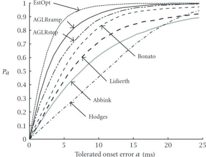
The accuracy function
Pa=Pˆt0−t0≤a (20)
shown in Figure 4 can be used as another measure of de-tection performance. The accuracy function denotes the per-centage of responses that were detected with an absolute error smaller than or equal to a maximum tolerated errorafor dif-ferent values ofa. For largea, the diagram reflects the general ability of a method to detect an onset, whereas a particular accuracy requirement of a method can specifically be assessed at small valuesa. Thus, the more a curve approaches the up-per left corner, the higher is the onset detection quality. As a major result, the accuracy functions in Figure 4 confirm the ranking already obtained from the PDFs shown in Figure 3.
Effect of signal to noise ratio
0 5 10 15 20 25 0
0.1 0.2 0.3 0.4 0.5 0.6 0.7 0.8 0.9 1
P
Tolerated onset error a
Bonato EstOpt
Hodges Lidierth
Abbink AGLRstep
AGLRramp
a
(ms)
Figure4: Accuracy functions of onset estimates (Mixed Trialsdata set). The ordinate value denotes the probability that the tolerated erroragiven by the abscissa value isnotexceeded. The further a curve is bent to the upper-left corner, the better is the onset detection quality.
usually adapted to the background activity (noise) and thus varies with SNR. The higher the noise level (decreasing SNR), the larger the threshold and, consequently, the later the onset will be detected.
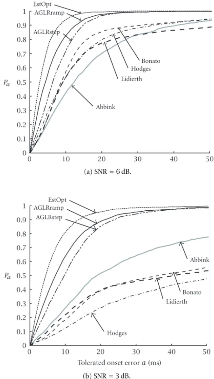
Degradation of performance with smaller SNR is partic-ularly obvious from the accuracy functions in Figure 6 (Fixed SNR Trials). For SNR = 6 dB, all methods provided accept-able results (see Figure 6a) but decreasing signal quality to SNR = 3 dB promptly reveals their specific quality and ro-bustness (see Figure 6b). The optimal referenceEstOptstill detects93% (SNR 6 dB) and 82% (SNR 3 dB) of all onsets with an accuracy of 10 ms.AGLRrampandAGLRstepfollow closely with a near-zero rate of undetected onsets. Even for the 3 dB trials, more than98%of onsets are detected with an abso-lute error less than 50 ms. But all the purely threshold-based methods (Abbink, Bonato, Lidierth, Hodges) cannot compete with likelihood-based methods; especially for the 3 dB situa-tion, their performance deteriorates extremely.
Effect of change dynamics
Figure 7 illustrates the dependence of mean onset error on ramp duration τ (Mixed Ramp Trials). AGLRramp is de-signed to compensate change dynamics, and, thus results are closest to those ofEstOpt. ButBonato, Lidierth, andAGLRstep show a similar small sensitivity to ramp duration, onlyAbbink andHodgesare rather sensitive. Variability of onset estimates (around mean onset error) was not affected by variations in ramp duration.
Generally, changing SNR predominately affects the onset error PDF width and the percentage of undetected (missed) onsets, whereas increasing ramp duration leads to a delayed onset detection (onset error bias).
6 7 8 9 10 11 12
2 4 6 8 10 12 14
Standar
d de
viation of
onset er
ror
(
ms
)
EstOpt Lidierth
AGLRstep Bonato
AGLRramp Abbink
Hodges
(a) Standard deviation of onset error.
6 7 8 9 10 11 12
0 5 10 15
M
ean onset er
ror
(
ms
)
SNR (dB)
Lidierth EstOpt
AGLRramp Abbink
AGLRstep
Hodges Bonato
− −
−5
10
15
(b) Mean onset error.
Figure5: Dependence of onset estimation error on signal-to-noise ratio (SNR) for theMixed SNR Trialsdata set (SNR 6–12 dB, ramp duration 20 ms).
4. EVALUATION OF DETECTION PERFORMANCE ON REAL SEMG RECORDINGS
4.1. Data acquisition
sub-0 10 20 30 40 50 0
0.1 0.2 0.3 0.4 0.5 0.6 0.7 0.8 0.9 1
Bonato EstOpt
AGLRramp
Hodges Lidierth
Abbink AGLRstep
Pa
(a)SNR=6dB.
Tolerated onset error a (ms)
0 10 20 30 40 50
0 0.1 0.2 0.3 0.4 0.5 0.6 0.7 0.8 0.9 1
Bonato EstOpt
AGLRramp
Hodges
Lidierth Abbink AGLRstep
Pa
(b)SNR=3dB.
Figure6: Dependence of accuracy functions on SNR for constant ramp duration of 20 ms.
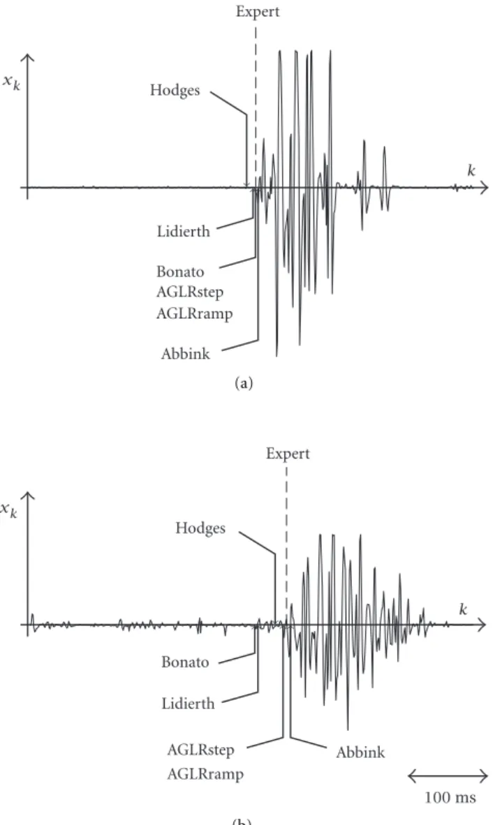
ject produced 120 single responses. The recorded data were visually inspected and only those responses which were def-initely initiated between 100 and 400 ms after stimulus pre-sentation were included to the test data set comprising a total number of 587 responses.
As a major handicap of real data, the true response onset t0is unknown and, therefore, the onset errorε=ˆt0−t0as
used before cannot be determined. But performance of the methods can be assessed on a relative basis; to this, the onset errorε=ˆt0−trefwas computed as the deviation between the
onset estimatesˆt0provided by the tested methods and the
onset estimatestref visually determined by a human expert.
In order to maximize the percentage of correct detection of the methods, their decision thresholds were set individually by taking the smallest valuehfor which the number of de-tected responses with alarm times−50≤ta−tref≤200ms
was maximum. The resulting thresholds are summarized in Table 3.
5 10 15 20 25 30
0 5 10 15
M
ean onset er
ror
(
ms
)
Ramp duration (ms)
EstOpt Lidierth
Abbink AGLRstep
Hodges Bonato
AGLRramp −5
−10
−15
−20
Figure7: Dependence of mean onset error on ramp duration. Eval-uation ofMixed Ramp Trialsdata set (SNR of 10 dB, ramp duration 5–30 ms).
Table3: Statistics for real SEMG data set.
Method Thresholdh Detectedonsets Meanerror ErrorSTD
AGLRramp 200 100.0% 0.4 ms 3.6 ms
AGLRstep 200 100.0% 0.5 ms 3.5 ms
Bonato 20 99.8% −0.8 ms 5.5 ms
Lidierth 3 99.5% −2.3 ms 6.9 ms
Abbink 30 98.6% −0.6 ms 9.8 ms
Hodges 5 99.0% −7.5 ms 9.3 ms
Bonato
AGLRramp Expert
Hodges
Lidierth
Abbink AGLRstep
k xk
(a)
Bonato
AGLRramp Expert
Hodges
Lidierth
Abbink AGLRstep
100 ms
xk
k
(b)
Figure8: Raw SEMG signals obtained in a reaction time experiment: two sample traces (a) and (b) with different SNR. Onset estimates of each method are indicated by markers. Dotted lines indicate the expert’s reference.
the small difference between theAGLRrampandAGLRstep algorithm indicating steep response profiles close to the step-like pattern of assumed by theAGLRstepmethod.
5. DISCUSSION
All methods perform well in detecting the onset time in good quality SEMG signals; thus, the difficulty to decide on the appropriate method appears with low SNR when SEMG sig-nals are disturbed for some reason. In any case, the choice is also dependent on implementation issues like method com-plexity, real-time implementation capability, and the required CPU performance.
Simple threshold-based methods are very popular be-cause of their intuitive and easy implementable structure. In
0 5 10 15 20 25
0 0.05 0.1 0.15 0.2 0.25 0.3 0.35 0.4 0.45
AGLRstep AGLRramp
Onset error (ms)
Bonato Abbink Lidierth
Hodges
−5 −10 −15 −20 −25
(a) Probability density functions of onset estimation errors.
0 5 10 15 20 25
0 0.1 0.2 0.3 0.4 0.5 0.6 0.7 0.8 0.9 1
P
Tolerated onset error a (ms) Bonato AGLRramp
Hodges Lidierth
Abbink AGLRstep
a
(b) Accuracy functions.
Figure9: Analysis of deviations between estimated change times and expert’s reference obtained on real SEMG signals with different computerized detectors.
most cases, SEMG signals have a good SNR, so these methods are well applicable with the main limitation that SNR should be larger than 10 dB. But SEMG of small and deep muscles as well as SEMG recorded in patients with neuromuscular diseases may not fit into this SNR requirement, which calls for application of more sophisticated approaches.
alarm time, the large variability of resulting change time esti-mates and their systematic dependence on change dynamics confine the application of simple threshold-based methods if SNR is low and/or highly accurate change time estimation is required.
Analysis of simulated as well as real SEMG data showed that appropriate signal conditioning of the measured raw SEMG is a prerequisite for high detection performance. Low-pass filtering the (full-wave-rectified) SEMG before com-puting the test function substantially reduces the risk of false alarms. But it causes a very smooth incline of the pre-processed signal near the onset and thus will lead to increased variability of estimated change times. Simple-threshold detectors likeHodgesare known for their results being very sensitive to the parameters of the lowpass filter used [13]. The Abbink approach suffers from this dilemma, too, despite of the more sophisticated change time estimation procedure.
Application of an adaptive pre-whitening filter proved to be superior to the less specific lowpass filter. Simulations with whiteGaussian SEMG signals have shown thatBonatoand Lidierth almost have the same onset error distribution, which is a consequence of their resembling detection strate-gies. Analysis of the more realistic colored SEMG data (see Figure 4) as well as analysis of real SEMG signals (see Figure 8) demonstrated the distinct performance gain of Bon-atodue to the use of an appropriate pre-whitening filter. Gen-erally, the implicit highpass characteristic of the whitening fil-ter preserves or even improves change dynamics as desired but accentuates the higher frequencies of possibly superimposed additive noise [22]. Therefore, we can expect good perfor-mance of the whitening filter provided that the noise is small compared to the variance profileσ2(k).
If higher robustness to changes in signal parameters and high detection precision is required, a pre-whitening filter together with a statistically optimized decision rule is the first choice. Consistently, the two model-based approaches AGLRstepandAGLRrampprovided higher detection power and more accurate change time estimates than the unspe-cific detectors both for the simulated and real SEMG signals. Particularly, these methods were most robust with respect to variations in signal properties such as SNR and change dy-namics. However, model-based approaches are usually asso-ciated with higher computational efforts, particularly, when the dynamic of the change is not known and has to be esti-mated from the data. Results show only minor loss of per-formance for the computationally more efficientAGLRstep algorithm compared to the more specific but more complex AGLRrampalgorithm. In order to reduce the computational effort of such more complex parametric detectors, a step-like stopping rule according to (31) may be combined with the ML change time estimator as shown in (37). This allows for an efficient implementation of the detection procedure, since the time-consuming estimation of the onset shape profile is only initiated once a change has been indicated.
An important aspect of computerized onset detection is post-processing. Generally, combining an arbitrary stop-ping rule with a post-processor testing multiple alarm/change
times for their plausibility can improve detection perfor-mance. Particularly, the detection threshold can be reduced since false alarms can be partly compensated by the post-processor. The use of an adequate post-processor is par-ticularly important when the SEMG signal contains mul-tiple changes indicating different levels of muscle activa-tion. In this case, the detection unit produces a sequence of change times indicating possible transitions between dif-ferent levels of muscle activation. A post-processor then groups the segments according to their variance merging segments with similar variance together. Combinations of GLR-based decision rules and post-processor have been suc-cessfully applied for the detection of pre-motor silent peri-ods in SEMG signals [22] and for the detection and classi-fication of events in the uterine EMG [23]. But any of the post-processors presented is also dependent on signal con-ditioning and alarm time generation. This means that any impairment caused by signal conditioning will nevertheless affect detection.
6. EPILOGUE: DESIGN, PRESENTATION, AND COMPARISON OF ALGORITHMS
“An algorithm must be seen to be understood and the best way to learn how an algorithm works is to play with it.” (Donald Knuth, in “The Art of Computer Programming,” [24]).
Every algorithm has embedded parameters, and it works only properly if these parameters are appropriately chosen. “Good” parameters are often determined by trial and error using simulated data. Despite the importance of finding and choosing the right parameters, usually little emphasis is de-voted to this step by papers about algorithms, presumably because there is no clear mathematical theory behind it (i.e., scientifically accepted).
The presentation of algorithms to the scientific commu-nity is usually done by writing about
(1) the practical and mathematical background, (2) a useful class of models,
(3) a description of the algorithm(s),
(4) a theoretical analysis of the behavior in some limiting cases,
(5) a table of numbers showing the performance of the al-gorithm tested on simulated data, while keeping some parameters in the signal model and the algorithm fixed,
(6) as in (4), but also with information about competing algorithms,
(7) a plot of a signal together with the corresponding output of the algorithms in question.
What typically is missing is a tool
(a) to check and interactively change the signal and to find good parameters for the algorithms for other ap-plications,
(c) to check the behavior of the algorithm(s) with real data.
These aspects are even more valid in the case of on-line algorithms. In the statistical community, new ways to present results using the internet were emphasized [25], and several groups are currently working on software tools which allow a user with any standard browser to visualize and change sig-nals and algorithms. To our experience, systematically but inductive trying of all the parameters in both the model and the algorithm yields quickly an idea about interesting neighborhoods in parameter space, quality, and stability of an algorithm. Software tools appropriate for this purpose should be easy to use and should not require a comprehensive instal-lation procedure: neither many researchers nor referees do have the time to reprogram a new algorithm in their own favorite programming environment to evaluate new signal processing procedures. To illustrate this point, an onset de-tection program designed in MATLAB*will be made avail-able to the readers by the authors, which allows to visual-ize the model described above, to change its parameters and to see the output of some selected algorithms. Using such tools simplifies to assess an algorithm or method, but requires to own a MATLAB* license up to now. But there are some developments to overcome this problem (e.g., compiler ver-sion) in near future, which will allow the software package to be made available through the internet.
APPENDIX
In this section, the implementation of the AGLRstep and AGLRrampdecision rules for the present signal model are shortly described.
The structure of the tests depends upon the variance pro-files before and after the response onsett0which, according
to the process model, are
σ2
0(k)=σnoise2 , (21)
σ2
1k, t0=σnoise2 +σsignal2 uk, t0, (22)
respectively. The variance patternσ2
0(k)before change (i.e.,
response onset) depends upon a single parameter
σ2
0k, θ0=θ0=constant, (23)
which is equal to the unknown variance σ2
noise. The ML
estimate ofθ0can be obtained from the initialMdata points
according to
Differentiation with respect toθ0and solving the resulting
likelihood equation
Thus, the estimated variance profile before change is equal to the average signal energy within the reference window.
Determination of the variance pattern σ2
1(k, j) after
change is more complicated since it depends upon the dy-namic change profileu(k, j)which, generally, is not known. This issue is addressed in the next paragraphs.
AGLRstep detector
The AGLRstep detector simply assumes an approximately constant variance profile of unknown magnitude θ1 after
change, that is,
σ2
1k, j, θ1=θ1=const. (27)
In this case, the log-likelihood ratio in (14) can be written as
ˆ
whereθˆ0is the estimated variance before change according
to (26). Maximization with respect toθ1is explicitly possible
by replacingθ1by its ML estimate
ˆ
Thus, theAGLRstepdecision rule can be summarized as
ta=mink≥W:gk≥h,
AGLRramp detector
TheAGLRrampdetector uses a more complex test function which also takes the dynamic change profile into account. It assumes that the shapeu(k, j)of the additive change in the variance profile is known but its exact magnitudeσ2
signal is
unknown, that is,
σ2
1k, j, θ1=θ0+θ1u(k, j). (33)
Then, the log-likelihood ratio in (14) can be rewritten as
ˆ
where the unknown magnitudeθ1is the only parameter to
be determined. Differentiating thelog-likelihood ratio with respect toθ1results in a likelihood equation which cannot be
explicitly solved. Therefore,θ1is estimated from the observed
sequence according to
by exploiting the statistical independence of the data se-quence. The resulting AGLR decision rule for the detection of an additive change with known dynamic profile but unknown magnitude is
whereθˆ1(j, k)is individually determined for each
combina-tion(j, k)according to (35).
If the exact profile is also unknown, the test may in-clude more maximizations which determine the ML esti-mates of the unknown parameters, too. Particularly,u(k, j) may be replaced by a set ofN template profilesu(k, j)(n), n = 1,2, . . . , N, together with an additional maximization which selects the most likely template according to
ˆ
TheAGLRrampalgorithm was implemented with parameters W = 25,h = 10,∆= 100,M = 200, and a set ofN = 8
shaping functions with ramp durationsτ=5,10, . . . ,40ms.
REFERENCES
[1] E. A. Clancy and N. Hogan, “Probability density of the surface electromyogram and its relation to amplitude detectors,”IEEE Trans.Biomed.Eng., vol. 46, pp. 730–739, 1999.
[2] J. H. Abbink, A. van der Bilt, and H. W. van der Glas, “De-tection of onset and termination of muscle activity in surface electromyograms,”J.Oral Rhabil, vol. 25, pp. 365–369, 1998. [3] S. V. Adamovich, M. F. Levin, and A. G. Feldman, “Merging
dif-ferent motor patterns: coordination between rhythmical and discrete single-joint movements,”Exp.Brain Res., vol. 99, pp. 325–337, 1994.
[4] P. Brodin, T. S. Miles, and K. S. Turker, “Simple reaction-time responses to mechanical and electrical stimuli in human masseter muscle,”Arch.Oral Biol., vol. 38, pp. 221–226, 1993. [5] S. A. V. M. Haagh, W. A. C. Spijkers, B. Van den Boogaart,
and A. Van Boxtel, “Fractioned reaction time as a function of response force,”Acta.Psychol., vol. 66, pp. 21–35, 1987. [6] J. K. Leader 3rd, J. R. Boston, and C. A. Moore, “A data
depen-dent computer algorithm for the detection of muscle activity onset and offset from EMG recordings,” Electroenceph.Clin. Neurophysiol., vol. 109, pp. 119–123, 1998.
[7] S. Micera, A. M. Sabatini, and P. Dario, “An algorithm for detecting the onset of muscle contraction by EMG signal pro-cessing,”Med.Eng.Phys., vol. 20, pp. 211–215, 1998.
[8] J. Nilsson, M. Panizza, and P. Arieti, “Computer-aided deter-mination of the silent period,” J.Clin.Neurophysiol, vol. 14, pp. 136–143, 1997.
[9] R. D. Rafal, A. Winhoff, J. H. Friedman, and E. Bernstein, “Pro-gramming and execution of sequential movements in Parkin-son’s disease,” J.Neurol.Neurosurg.Psychiatry, vol. 50, pp. 1267–1273, 1987.
[10] K. Takada and K. Yashiro, “Automatic measurement of on/off periods of EMG activity,”Medinfo, vol. 8, pp. 751–754, 1995. [11] G. J. M. van Boxtel, L. H. D. Geerats, M. M. C. Van den
Berg-Lenssen, and C. H. M. Brunia, “Detection of EMG onset in ERP research,”Psychophysiology, vol. 30, pp. 405–412, 1993. [12] G. Staude and W. Wolf, “Objective motor response onset
de-tection in surface myoelectric signals,”Med.Eng.Phys., vol. 21, pp. 449–467, 1999.
[13] P. W. Hodges and B. H. Bui, “A comparison of computer-based methods for determination of onset of muscle contraction us-ing electromyography,”Electroenceph.Clin.Neurophysiol., vol. 101, pp. 511–519, 1996.
[14] P. Bonato, T. D’Alessio, and M. Knaflitz, “A statistical method for the measurement of muscle activation intervals from sur-face myoelectric signal during gait,”IEEE Trans.Biomed.Eng., vol. 45, pp. 287–298, 1998.
[16] G. Staude, R. Dengler, and W. Wolf, “The discontinuous nature of motor execution part I: a model concept for single-muscle multiple-task coordination,”Biol.Cybern., vol. 82, pp. 23–33, 2000.
[17] L. Ljung,System Identification: Theory for the User, Prentice-Hall, New Jersey, 1987.
[18] G. Barrett, H. Shibasaki, and R. Neshige, “A computer-assisted method for averaging movement-related cortical potentials with respect to EMG onset,”Electroenceph.Clin.Neurophysiol., vol. 60, pp. 276–281, 1985.
[19] H. G. Choi, J. C. Principe, A. A. Hutchison, and J. A. Woz-niak, “Multiresolution segmentation of respiratory elec-tromyographic signals,”IEEE Trans.Biomed.Eng., vol. 41, pp. 257–266, 1994.
[20] G. Staude, W. Wolf, and U. Appel, “Automatic event detection in surface EMG of rhythmically activated muscles,” An Int. Conf.IEEE BME Soc., vol. 17, pp. 1351–1352, 1995.
[21] G. Staude and W. Wolf, “Voluntary motor reactions: does stimulus appearance prolong the actual tremor period?,” J. Electromyogr.Kinesiol., vol. 9, pp. 277–281, 1999.
[22] G. Staude, V. Kafka, and W. Wolf, “Determination of premotor silent periods from surface myoelectric signals,”Biomed.Tech., vol. 45, no. 2, pp. 228–232, 2000.
[23] M. Khalil and J. Duchêne, “Uterine EMG analysis: a dynamic approach for change detection and classification,”IEEE Trans. Biomed.Eng., vol. 47, pp. 748–756, 2000.
[24] D. E. Knuth, The Art of Computer Programming, Addison-Wesley, Massachusetts, 1998.
[25] W. West, T. Ogden, and A. Rossini, “Statistical tools on the WWW,”The American Statistician, vol. 52, pp. 257–262, 1998.
Gerhard Staude received the M.S.E.E. in 1990 from the Technical University Munich, Germany, and the Ph.D. degree in electrical engineering in 1996 from the University of the Armed Forces at Munich, Germany. From 1996 to 1997 he was a member of the interdis-ciplinary graduate college “Sensory Interac-tion in Biological and Technical Systems” of the Deutsche Forschungsgemeinschaft. Cur-rently, he is affiliated with the Department of
Electrical Engineering at the University of the Armed Forces, where he heads the Neuromuscular system research group at the Institute of Mathematics and Computer Science. He is author of more than 30 refereed journal papers in the fields of digital signal processing and analysis of the human motor system. His major research inter-ests include parameter estimation and change detection in motor-related biosignals, and basic research in the human motor system with special focus on biological oscillators (e.g., physiological and pathological tremors) and movement coordination.
Claus Flachenecker received his M.S.E.E in 1994. He continued as a Ph.D. student at BMW AG, Munich, in cooperation with the Technical University Munich, Lehrstuhl für Elektrische Meßtechnik. This work com-prised intense cooperation with the Euro-pean STAUMECS and German ASAM stan-dardization groups, that define plug & play integration standards for product testing en-vironments. After receiving his Ph.D. degree
in 1998, he was affiliated with the University of the Armed Forces at Munich to research biosignal related topics, set-up a driving simula-tor environment with incorporated physiological driver monisimula-toring
and create intelligent feedback controllers to be used in force-feedback pedals for automobiles. Since end of 2000, he is working for Carl Zeiss Ophthalmic, Inc. (California, USA), as a systems design engineer. His responsibilities now include the design and develop-ment of diagnostic medical devices for the eye-care industry.
Martin Daumer received the diploma in Physics in 1990 and the Ph.D. in mathe-matics both from the Ludwig-Maximilians-University Munich, Germany in 1995. In 1987 he was a summer student at CERN, Geneva, and in 1992 he spent one year with a stipend of the DAAD at the Department for Mathematics at the Rutgers University, New Jersey. From 1993–1996 he was a mem-ber and later post-doc of the interdisciplinary
graduate college “Mathematics in its relationship with Physics” from the Deutsche Forschungsgemeinschaft DFG. Since 1996 he is head-ing the Research group “Online Monitorhead-ing in Medicine” in cooper-ation with the Sonderforschungsbereich 386 “Statistical Analysis of Discrete Structures” at the Institute for Medical Statistics and Epi-demiology of the Technical University of Munich. He has published more than 40 articles about topics in quantum physics, scattering theory, probability theory, biosignal processing and holds patents for methods and devices for change-point detection and internet-based monitoring of biosignals. In 1999 he founded the IT-company Trium Analysis Online, which is playing a central role in various na-tional (BMBF) and internana-tional research projects, for example, the Sylvia Lawry Centre for Multiple Sclerosis Research.
Werner Wolfreceived his M.S.E.E. in 1970 and his Ph.D. in 1978, both from the Tech-nical University Munich, Germany. Now, he is a member of the Faculty of Electrical En-gineering of the University of the Armed Forces at Munich. From 1970 to 1978, he was engaged in an interdisciplinary research project “Visual Perception” of the Institute of Communication Systems, Technical Univer-sity Munich, with special focus on the