Cyclic Codes: Low-Weight Codewords and Locators

U

NIVERSITY OF

TRENTO

D

EPARTMENT OF

M

ATHEMATICS

P

HD

IN

MATHEMATICS

XXVIII C

YCLE

Cyclic Codes: Low-Weight Codewords

and Locators

Author:

Claudia T

Advisor:

Prof. Massimiliano S

Head of the Doctoral School:

Prof. Valter M

1 Introduction 1

1.1 Objectives and Contributions . . . 1

1.1.1 Finding Low-weight codewords . . . 1

1.1.2 Decoding cyclic codes . . . 2

1.2 Thesis Organization . . . 3

I

Preliminary results

5

2.2 Some Notions in Complexity Theory . . . 8

2.2.1 Basic notions . . . 8

2.2.2 Theory of NP-Completeness . . . 10

2.3 Basic Notions in Finite Fields . . . 12

2.4 Linear Recurring Sequences . . . 17

2.5 Discrete Logarithms . . . 18

2.5.1 Computing Discrete Logarithms . . . 19

2.5.2 Zech Logarithm Table . . . 22

3 Decoding Problem for Cyclic Codes 25 3.1 An overview on error correcting codes . . . 25

3.2 Linear Codes . . . 28

3.2.1 Basic definitions . . . 28

3.2.2 Decoding Linear Codes . . . 31

3.3 Cyclic Codes . . . 33

3.3.1 Basic definitions . . . 33

3.3.2 Decoding Cyclic Codes . . . 37

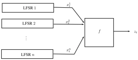
4 Correlation Attacks on LFSR-based Stream Ciphers 49 4.1 Preliminaries . . . 49

4.1.2 Boolean functions . . . 50

4.1.3 Birthday Problem . . . 52

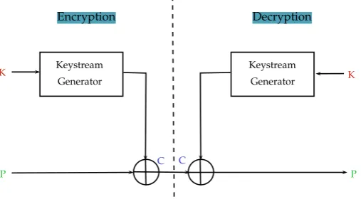
4.2 Stream ciphers . . . 55

4.2.1 Standard properties of keystream sequences . . . 55

4.2.2 LFSR-based stream ciphers . . . 57

4.3 Correlation attacks on LFSR-based stream ciphers . . . 59

4.3.1 Correlation attacks . . . 60

4.3.2 Fast correlation attacks . . . 61

II

Main results

65

5.2 The algorithm . . . 72

5.2.1 Description of Algorithm 3 . . . 72

5.2.2 Complexity estimates . . . 74

5.3 Significant Examples . . . 77

6 On the shape of the general error locator polynomial 79 6.1 A new representation of the locator polynomial . . . 79

6.2 Sparse locators for some classes of codes witht= 2. . . 83

6.3 Sparse locators for some classes of codes witht= 3. . . 90

6.4 On the complexity of decoding cyclic codes . . . 98

6.4.1 Complexity of the proposed decoding approach . . . 98

6.4.2 Comparison with other approaches . . . 101

III

Appendices

105

B.2 Binary cyclic codes witht = 3 . . . 114

B.3 Some classes of binary cyclic codes presented in Chapter 6 . . . 117

Introduction

Error correcting codes has become an integral part of the design of reliable data transmis-sions and storage systems. Their employment in these applications provide mechanisms for the detection and correction of errors. Error correcting codes are also playing an increasingly important role for other applications such as the analysis of pseudorandom sequences and the design of secure cryptosystems. Cyclic codes form a large class of widely used error correct-ing codes, includcorrect-ing important codes such as the Bose-Chaudhuri-Hocquenghem (BCH) codes, quadratic residue (QR) codes and Golay codes. Cyclic codes were studied first by E. Prange in 1957 [Pra57], who discovered their rich algebraic structure. Their extensive employment in real-life applications is due to two main aspects: they offer powerful error detection and cor-rection capabilities and possess algebraic properties permitting the use of simplified processing procedures and a much easier investigation when compared to non-cyclic codes. For instance, the encoding of data into cyclic code words can easily be achieved in hardware using a simple linear feedback shift register. Currently, the main drawback of cyclic codes is the lack of an efficient decoding algorithm for them.

1.1

Objectives and Contributions

This thesis is devoted to two problems arising in the study of cyclic codes: finding low-weight codewords and decoding. In the rest of this section we briefly describe where our con-tribution is positioned and point out the main results of the thesis.

1.1.1 Finding Low-weight codewords

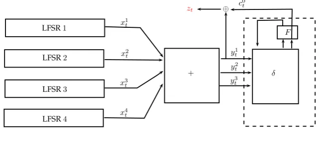
different approaches, one based on the birthday paradox [CJM02] and another based on discrete logarithms [DLC07]. A cipher like E0 ([GPS04]) is not immediately subject to these types of attacks, since no apparently single LFSR is correlated to the keystream output. In [LV04], Lu and Vaudenay introduced a new fast correlation attack (often called faster correlation attacks) which is able to successfully recover the state of E0. Their attack requires a different precompu-tation step which computes a single parity check of multiple LFSRs. Since the data complexity of the attack is bounded from below by the degree of the parity check, one tries to find a parity check of degree less than a target degree. The complexity of their precomputation step is not far from the complexity of their full attack, and they employed the generalized birthday approach presented in [Wag02]. In Chapter 5 an alternative approach for solving this problem based on discrete logarithms is described. In some interesting cases our algorithm has a time complexity comparable to the generalized birthday approach, while having a much lower memory com-plexity (i.e. O(1)). These cases are relevant to faster correlation attacks to a class of stream

ciphers (including the Bluetooth cipher E0) and when the polynomial is the product of many irreducible factors. The design of the new algorithm has been published [PST16].

1.1.2 Decoding cyclic codes

In the last fifty years many efficient bounded-distance decoders have been developed for special classes of cyclic codes, e.g. the Berlekamp-Massey (BM) algorithm ([Mas69]) designed for the BCH codes. Although BCH codes can be decoded efficiently, it is known that their de-coding performance degrades as the length increases ([LW67]). Cyclic codes are not known to suffer from the same distance limitation, but no efficient bounded-distance decoding algorithm is known for them (up to their actual distance).

In [OS05] Orsini and Sala introduced the general error locator polynomial and presented an algebraic decoder which permits to determine the correctable error patterns of a cyclic code in one step. They constructively showed that these polynomials exist for any cyclic code (it is shown to exist in a Gröbner basis of the syndrome ideal), and gave some theoretical results on the structure of such polynomials in [OS07], without the need to actually compute a Gröb-ner basis. They also provide a structure theorem for these locators for a class of binary cyclic codes, which has been generalized by Chang and Lee [CL10] for binary cyclic codes that could be defined by only one syndrome. In Chapter 6 a generalization of this result is showed, along with several results for infinite classes of binary cyclic codes witht= 2andt= 3. From these,

a theoretically justification of the sparsity of the general error locator polynomial is obtained for all binary cyclic codes witht _≤ 3andn < 63, except for three cases where the sparsity is

1.2. Thesis Organization

1.2

Thesis Organization

The remainder of the thesis is structures in three parts.

Part I: Background

In this part we aim to introduce and motivate our research objectives. We also provide some preliminary results which we will use in Part II. This part does not contain original contributions. It is organized as follows:

Chapter 2

In this chapter we review some well-known results in arithmetics, in complexity theory and in finite field theory that will be used along the thesis. Particular focus is directed towards fundamental properties of polynomials over finite fields and discrete logarithms computation.

Chapter 3

In this chapter the study of error correcting codes is introduced. Basic properties of linear codes are presented, and it is discussed the complexity of the decoding problem for these codes. The algebraic structure of cyclic codes is described and the problem of decoding cyclic codes is addressed. Established decoding techniques for BCH codes are presented along with their complexity. Finally, general error locators for cyclic codes are introduced, and it is discussed some promising properties of these locators for decoding cyclic codes.

Chapter 4

In this chapter basic notions in Cryptography and current algorithms for solving the Gen-eralized Birthday Problem are briefly reviewed. Some basic properties of LFSR-based stream ciphers, their security level and the standard procedures for achieving a good level of security are described. Finally, correlation attacks and fast correlation attacks on LFSR-based stream ciphers are introduced.

Part II: Contributions

This part is devoted to our original results. It is organized as follows:

Chapter 5

birthday approach and to the straightforward generalization of the discrete log approach for the case of a single primitive polynomial. Significant examples of our approach are outlined in the final part of the chapter, where we show that for the fast correlation attack in [LV04] our algo-rithm could be more convenient to use in the second precomputation step than the generalized birthday approach, and that the method we propose is substantially better than the generalized birthday approach in the case where the polynomial can be decomposed in several irreducible factors, each one of degree less than20. This chapter is based on a journal publication [PST16].

Chapter 6

In this chapter we deal with some issues concerning the efficiency of the Orsini-Sala bounded-distance decoding algorithm based on general error locators for cyclic codes. A new result on the structure of the general error locator polynomial for a class of cyclic codes is obtained, and it is shown sparse general error locator polynomials for infinite classes of binary cyclic codes with error correction capabilityt_≤3, adding theoretical evidence to the sparsity of this locator

for infinite classes of codes. Finally, the complexity of bounded-distance decoding of certain classes of cyclic codes is studied.

Part III: Appendices

This part contains two appendices.

• Appendix A includes two tables. The first table lists the binary cyclic codes witht = 3

andn <63, while the second table reports a general error locator polynomial for binary

cyclic codes witht= 3andn = 55.

Part I

Algebraic and Complexity Background

In this chapter we fix some notations and report well-known results in arithmetics, in com-plexity theory and in finite field theory that will be used along the thesis.

For this chapter definitions and results are mainly from [LN97, Knu81, GJ79, MP13, MM07, MBG+_{13, Mor03].}

2.1

Modular Arithmetic

In a Euclidean ring, we denote by amodc the remainder of the division of a by c. We

write a _≡ b (mod c) if a is congruent to b modulo c. We denote by LCM and GCD the

Least Common Multiple and the Greatest Common Divisor — respectively — of polynomials or integers, depending on its inputs.

Definition 2.1.1. Letaandnbe integers withn >0andGCD(a, n) = 1. The smallest positive

integerkwithak_{≡1 mod nis called themultiplicative order of amodulonand is denoted by} ordn(a).

Note that, as a consequence of Euler’s theorem, ordn(a) always divides ϕ(n), ϕ being the

Euler’s function.

Definition 2.1.2. Letaandnbe positive integers withGCD(a, n) = 1, and letibe an integer

with0_≤i < n. The set

Ci ={i, ia, ia2, . . . , ias−1},

wheresis the smallest positive integer withias_≡i (mod n), is said thecyclotomic coset of a

(ora-cyclotomic coset)moduloncontainingi.

The distincta-cyclotomic cosets modulonpartition the set of integers

[0, n₋1] :=_{0,1, . . . , n₋1_}.

A subset{i1, . . . , is}of[0, n−1]is called acomplete set of representativesof cyclotomic cosets

ofamodulon ifCi1, . . . , Cis are distinct and

Ss

j=1Cij = [0, n−1]. Note that ordn(a)is the size of thea-cyclotomic cosetC1modulon.

Theorem 2.1.3(Chinese Remainder Theorem). Letm1, m2, . . . , mr be positive integers which are relatively prime in pairs, i.e.

GCD(mj, mk) = 1 when j 6=k.

Let m = m1m2· · ·mr, and let a, u1, u2, . . . , ur be any integers. Then, there is exactly one integeruwhich satisfies the conditions

a_≤u < a+m, u_≡uj (mod mj), 1≤j ≤r.

We are interested in the following generalization of Theorem 2.1.3.

Theorem 2.1.4 (Generalized Chinese Remainder Theorem). Let m1, m2, . . . , mr be positive integers. Letm= LCM(m1, m2, . . . , mr), and leta, u1, u2, . . . , urbe any integers. Then, there is exactly one integeruwhich satisfies the conditions

a _≤u < a+m, u_≡uj (mod mj), 1≤j ≤r

provided that

ui ≡uj (mod GCD(mi, mj)), 1≤i < j ≤r.

We will denote by CRT(u1, u2, . . . , ur, m1, . . . , mr) the result of applying the (Generalized)

Chinese Remainder Theorem to integersui and modulimi.

2.2

Some Notions in Complexity Theory

In this section we recall some notions from computational complexity theory. Since it is not within our scope to deal with details of computational complexity, most of our definitions will be informal. For more details we refer the reader to [GJ79].

2.2.1 Basic notions

The goal of computational complexity theory is to measure the difficulty of problems. By aproblem, we mean a general question to be answered. A problem whose answer, orsolution, is “yes” or “no”, is called adecision problem. A problem usually possesses severalparameters whose values are left unspecified. Aninstanceof a problem is achieved by specifying values for those parameters.

Example 2.2.1. Consider the following problem

Problem (PRIME)

Input: An integern_≥2 Question: Isnprime?

The problemPRIMEis an example of decision problem having one parametern. An instance

2.2. Some Notions in Complexity Theory

Notice that, given a problem, there are many ways in which its instances can be described. We assume that for each problem one particular way has been chosen in advance. The func-tion which maps the problem instances into the strings describing them is called theencoding schemeof the problem. Theinput lengthfor an instanceI of a problemΠis defined to be the

number of symbols in the description ofI obtained from the encoding scheme forΠ.

A general step-by-step procedure, solving a problem, in a finite number of steps is called an algorithm.

The difficulty of a problem is measured by examining algorithms to solve it. The (worst-case) time complexityfor an algorithm expresses its time requirements by giving, for each possible input length, the largest amount of time needed by the algorithm to solve a problem instance of that size. The time complexity function of an algorithm is usually denoted byT(n), withnthe

input length.

Note that, depending on the assumptions, may be necessary consider separately thespace com-plexity of an algorithm, which is the number of registers used in the course of the algorithm. This is not essential for single-tape Turing machine, whose running time combines the time and memory complexity. A very significant fact about Turing machines is that any algorithm can be modeled by a Turing machine program. However, for a general algorithm writing such a program is a notably time-consuming task.

Different algorithms may have very different time complexity functions. One would like to characterize which of these algorithms are “too inefficient”, or “ intractable”, and which are “tractable”. Computer scientists recognize a simple distinction that offers considerable insight into these issues.

Definition 2.2.2(Big O Notation). Letf, g : _{N → R}+ be two positive real-valued functions.

We say thatf isO(g(n))if there a positive constantcand an integern0 such that

f(n)< c_·g(n), (2.1)

for all values ofn_≥n0.

Apolynomial time algorithmis defined to be one whose time complexity function isO(p(n))

for some polynomial functionp, where ndenotes the input length. Any algorithm whose time

complexity function cannot be so bounded is called anexponential time algorithm. We shall refer to a problem asintractableif no polynomial time algorithm can possibly solve it.

Arandomized algorithmis one wherein certain decisions are made based on the outcomes of coin flips made in the algorithm. Byprobabilistic polynomial time algorithm, we mean a randomized algorithm whose time complexity function is bounded by a polynomial in the size of the input.

Definition 2.2.3. We define

wheren is the size of the input space,0 _≤ γ _≤ 1, cis a constant andlnn denotes the natural

logarithm.

Let A be an algorithm. Denote with T(n) its time complexity function. We note that if

T(n) = L[n,0, c] then _A is a polynomial time algorithm, while if T(n) = L[n,1, c] then A is an exponential time algorithm. We say that A is a subexponential time algorithm if

T(n) = L[n, γ, c]with0< γ <1.

2.2.2 Theory of NP-Completeness

The theory of complexity is designed to be applied only to decision problems. The reason is that they possess useful properties allowing a better understanding of their complexity than non-decision problems. Moreover, most problems can be reduced to decision problems.

An important class of decision problems is the class P. We say that a decision problem Π

belongs toP ifΠis a polynomial-time algorithm. Another important class of decision problems

is the class NP. In order to introduce this class let us first consider the following example.

Example 2.2.4. The problem PRIME in Example 2.2.1 is an example of problem in the class

P. A (deterministic) polynomial time algorithm solving it, is the AKS primality test [AKS04].

Let us examine the following problem

Problem (THREE DIMENSIONAL MATCHING)

Input: A subsetU _⊆T _×T _×T, whereT is a finite set

Question: Is there a set W _⊆ U such that _|W_| = _|T_|, and no two elements of W agree in

any coordinate?

No polynomial time algorithm is known for solving theTHREE DIMENSIONAL MATCHING. However, suppose someone claimed, for a particular instance (T, U)of this problem, that the

answer for that instance is “yes” providing us with a setW which satisfies the property. It is

reasonable to expect that the problem of verifying the truth or falsity of such a claim, would be easier than the problem itself. It can be seen that for theTHREE DIMENSIONAL MATCHING this verification problem can be solved with a polynomial time algorithm. The class NP captures this notion of polynomial time verifiability.

An algorithm is said deterministic if its computation is fully determined by its input. An algorithm is nondeterministic if it is not deterministic, that is, if there may be more than one computation for a given input.

A nondeterministic algorithm is composed of two stages:

1. Guessing stage (nondeterministic): Given a problem instance I, some structure S is

“guessed”. Scan be thought of as a candidate solution of the problem for the instanceI.

2. Verification stage(deterministic): Taken as inputI andS, it returns “yes” if the candidate

2.2. Some Notions in Complexity Theory

LetΠbe a decision problem. Denote withDΠthe set of instances ofΠ. We say that an instance

I _∈ DΠ is an yes-instanceof Π if the solution of Π when particularized to the instance I is

“yes”. We denote the set of all yes-instances ofΠwithYΠ.

A nondeterministic algorithm is said to solve a decision problemΠif for all instancesI _∈DΠ:

• IfI _∈YΠ, then there exists some structureSthat, when guessed for inputI, will lead the

verification stage to respond "yes" forIandS.

• If I /_∈ YΠ, then there exists no structureS that, when guessed for inputI, will lead the

verification stage to respond "yes" forIandS.

In the complexity investigation of a decision problemΠ, one is usually interested in showing

that a polynomial-time algorithm exists forΠor thatΠis NP-complete.

A decision problemΠbelonging in NP is said an NP-complete problemif a polynomial-time algorithm for Π would yield a polynomial-time algorithm for every decision problem in the

class NP. A decision problem which has this property but is not necessary in NP is called an NP-hard problem.

The concept of NP-completeness was introduced in 1971 by Cook [Coo71] which also provided the first known NP-complete problem. Since the class NP is known to contain many problems that are considered computationally hard, the NP-completeness of a problemΠis considered as

a strong evidence suggesting thatΠdoes not admit a polynomial-time algorithm. Today a wide

variety of problems are known to be NP-complete. Note that, once we have at least one known NP-complete problem available, a straightforward method for proving that a decision problem

Πis NP-complete consists in showing that

• Π _∈N P;

• some known NP-complete problemΠ0 can be transformed with a polynomial time

trans-formation inΠ.

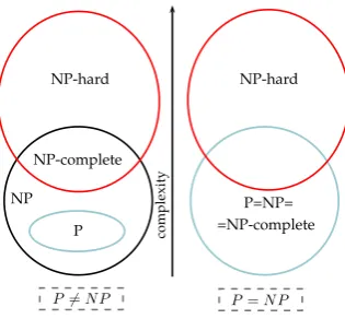
NP-hard

NP-complete NP

P

P=NP= NP-hard

=NP-complete

P6=N P P=N P

co

m

pl

ex

it

y

Note also that, trivially,P _⊆N P. On the contrary, whether or notN P _⊆P is one of the major

unsolved problems in computer science. Figure 2.1 shows a diagram of complexity classes under the two assumptions thatP ₆=N P andP =N P.

2.3

Basic Notions in Finite Fields

We denote by Fq the field ofq elements, whereq is a power of a prime p, by F∗q the

mul-tiplicative group of non-zero elements ofFq, byFq the algebraic closure of Fq, and by Fqnthe

standardn-dimensional vector space over_Fq.

In this section we recall some of the basic properties of finite fields.

Definition 2.3.1. A subset _K of a field _F that is a field under the operations of _F is called a subfieldofF, and we write_K⊆F. In this context,_Fis a called anextensionofK. IfM is any

subset of F, then the fieldK[M]is defined as the intersection of all subfields of F containing bothKandM. For finiteM ={θ1, . . . , θn}, we writeK(θ1, . . . , θn).

Proposition 2.3.2. Let _Fq be a finite field withq = ps. Every subfield of Fq haspm elements for some integerm dividings. Conversely, for any integer m dividings there exists a unique subfield of_Fqwithpm elements.

LetFq[x]be the ring of univariate polynomials overFq.

Definition 2.3.3. Let f _{∈ F}q[x]. The coefficient of the highest power ofx in f is called the

leading coefficientoff. We say thatf ismonicif its leading coefficient is1.

Definition 2.3.4. Letθ _{∈ F}qr andf(θ) = 0wheref(x)is a monic polynomial in _Fq[x]. Then

f(x)is called theminimal polynomialofθover_Fqifθis not a root of any nonzero polynomial

inFq[x]of lower degree.

Definition 2.3.5. A polynomial f _{∈ F}q[x] is an irreducible polynomial over _Fq if f has a

positive degree andf =ghwithg, h_∈Fqimplies that eitherg orhis a constant polynomial.

Proposition 2.3.6. Let θ _{∈ F}qr and f(x) be its minimal polynomial over _Fq. Then f is an irreducible polynomial.

Definition 2.3.7. Letf be a non-zero polynomial in_Fq[x]. Iff(0) 6= 0, then the order of f is

the least positive integerN such that1 +xN is a multiple off, and we denote it byord(f).

Proposition 2.3.8. Let f be a polynomial in_Fq[x]of positive degree and f(0) ₆= 0. Letf =

fb1

1 · · ·frbr, whereb1, . . . , br ∈ Nandf1, . . . , fr are distinct irreducible polynomials of degree

n1, . . . , nr, be the factorization off inFq[x]. Then,

1. ord(f) = qt_LCM(ord(f

2.3. Basic Notions in Finite Fields

2. Iffiis irreducible, thenord(fi)|qni−1;

Definition 2.3.9. Letf _∈Fq[x]of degreen. We say thatf isprimitiveiford(f) = qn−1.

Note that by point 2. of Proposition 2.3.8 we have that any primitive polynomial is irreducible.

Definition 2.3.10. Let f _{∈ F}q[x] be monic and of positive degree and F be an extension of

Fq. Then f is said to split in F if can be factored as a product of linear factors in F[x], i.e.

f(x) = (x₋α1)· · ·(x−αn). The field Fis asplitting field off overFq iff splits inFand F=Fq(α1, . . . , αn).

Proposition 2.3.11(Existence and Uniqueness of Splitting Field). Letf _∈Fq[x]be monic and of positive degree. Then there exists a splitting field off over_Fq. Moreover, any two splitting fields off over_Fqare isomorphic.

Next theorem summarizes some fundamental properties of finite fields

Theorem 2.3.12. Let_Fqbe a finite field withq=ps. Then

1. (a+b)pk

=apk

+bpk

fora, b_∈Fqandk ∈N

2. everya _∈Fqsatisfiesaq =a.

3. xq_{−1factors in}

FqasQ_a∈_F∗

q(x−a)

4. _Fq is isomorphic to the splitting field ofxq−xoverFp

5. _F∗_q is a cyclic group

Definition 2.3.13. An elementθ_∈Fqwhich multiplicatively generates the groupF∗qis called a primitive element.

Proposition 2.3.14. Let_Fq be a finite field, nbe an integer with GCD(n, q) = 1, andFqm be the splitting field ofxn_−1over

Fq. Then there exists an elementα ∈Fqmsuch that

xn₋1 = n−1

Y

i=0

(x₋αi). (2.2)

A such elementαis called a primitiventh root on unity over_Fq.

Definition 2.3.15. Let_Fqm be an extension of_Fq. An automorphism of _Fqm is said to be an automorphism of _Fqm over _Fq if it fixes the elements of _Fq. If α ∈ _Fqm, then the elements

α, αq_{, . . . , α}qm−1

are called theconjugatesofαwith respect to_Fq.

Proposition 2.3.16. The distinct automorphisms of _Fqm over_Fqare exactly the functions

f0,f1,. . .,fm−1, where

fj(α) =αq

j

for α _∈Fqm,

for0_≤j _≤m₋1. The functionf1is called the Frobenius automorphism ofFqm over_Fq.

Theorem 2.3.17. Let _Fq be a finite field andFqm be the splitting field of xn−1 over_Fq. Let

α_∈Fqm be a primitiventh root of unity over_FqwithGCD(n, q) = 1. Then

• For each integeriwith0_≤i < n, the minimal polynomial ofai over_Fqis

mαi(x) =

Y

j∈Ci

(x₋αj)_∈Fq[x],

whereCi is theq-cyclotomic coset moduloncontainingi.

• The conjugates ofαi _{are the elementsα}s _withs∈C i.

• The polynomialxn₋1has the factorization into monic irreducible polynomials over_Fq

xn₋1 = Y i

m_αi(x),

whereiruns through a set of representatives of theq-cyclotomic cosets modulon.

An important property of finite fields is that every function defined on a finite field can be realized by a polynomial with coefficients in that field. It is remarkable that this property characterizes finite fields in the sense finite fields are the only commutative ring with identity satisfying it. The next result tell us how to obtain a polynomial representing a given function over a field.

Theorem 2.3.18 (Lagrange Interpolation Formula). For n _≥ 0, let a0, a1, . . . , an be n + 1 distinct elements of a field_F, and letb0, b1, . . . , bnben+ 1arbitrary elements inF. Then there exists exactly one polynomial f _{∈ F}[x] of degree_≤ n such that f(ai) = bi for i = 0, . . . , n. This polynomial is given by

f(x) = n

X

i=0

bi n

Y

k=0

k6=j

(ai−ak)−1(x−ak).

For finite fields we can do somewhat better.

Theorem 2.3.19. Every function f : _Fq → Fq can be represented by a unique polynomial over _Fq of degree at most q−1, i.e there exist exactly one polynomial P ∈ Fq[x] such that

P(a) =f(a)for alla_∈Fq. Moreover such a polynomial is given by

X

a∈Fq

f(a) 1₋(x₋a)q−1

2.3. Basic Notions in Finite Fields

The previous result can be extended to functions with any number of variables.

Theorem 2.3.20. For any integer r _≥ 1, let f : _Fr_{q → F}q. Then f can be represented by a unique polynomialP _∈Fq[x1, . . . , xr]of degree at mostq−1in each variable. Moreover, such a polynomial is given by

X

(a1,...,ar)∈Frq

f(a1, . . . , ar)

Y

1≤i≤r

1₋(xi−ai)q−1

.

Definition 2.3.21. Let f _{∈ F}q[x1, . . . , xn]given byf(x1, . . . , xn) = Pai1...inx

i1

1 · · ·xinn with

n _≥ 1. If ai1...in 6= 0, thenai1...inx

i1

1 · · ·xinn is called atermoff andi1 +· · ·+inis called the

degree of the term. Forf ₆= 0, we define thedegreeoff, denoted bydeg(f), as the maximum

of the degrees of the terms off. Forf = 0we setdeg(f) = _−∞. Iff = 0or if all terms off

have the same degree, thenf is calledhomogeneous.

An important class of polynomials innvariables we will treat in Chapter 6 is that of

sym-metric polynomials.

Definition 2.3.22. Let f _{∈ F}q[x1, . . . , xn]. We say that f is symmetric if f(xi1, . . . , xin) =

f(x1, . . . , xn)for any permutationi1, . . . , inof the integers1, . . . , n.

Example 2.3.23. Let z be a variable over _Fq[x1, x2, . . . , xn], and let g(z) = (z − x1)(z −

x2)· · ·(z−xn). Then

g(z) =zn₋σ1zn−1+σ2zn−2+· · ·+ (−1)nσn, (2.3)

where

σk =σk(x1, . . . , xn) =

X

1≤i1<···<ik≤n

xi1· · ·xik, k = 1,2, . . . , n. (2.4)

Sinceg remains unchanged under any permutation of thexj, then the polynomialsσk are

sym-metric polynomials. Moreover, by definition, they are homogeneous.

Definition 2.3.24. For k = 1,2, . . . , n, the polynomial σk defined by (2.4) is called the kth elementary symmetric polynomialin the variablesx1, . . . , xnoverFq.

Theorem 2.3.25(Fundamental Theorem on Symmetric Polynomials). For any symmetric poly-nomialf _{∈ F}q[x1. . . , xn] there exists a uniquely determined polynomial h ∈ Fq[x1, . . . , xn] such that

f(x1, . . . , xn) =h(σ1, . . . , σn).

Definition 2.3.26. Fork _≥ 1, the polynomialxk

Theorem 2.3.27(Newton’s identities). Letσ1, . . . , σnbe the elementary symmetric polynomials in the variables x1, . . . , xn over Fq, and let s0 = n ∈ Z andsk = sk(x1, . . . , xn)be the kth power sum polynomials in the variables x1, . . . , xn over Fq for k ≥ 1. Then the following formula holds fork _≥1

sk−sk−1σ1 +sk−2σ2+· · ·+ (−1)m−1sk−m+1σm−1+ (−1)m

m

nsk−mσm = 0,

wherem= min(k, n).

Theorem 2.3.28(Waring’s Formula). With the same notation as Theorem 2.3.27, fork _≥1, we have that

sk=

X

(₋1)i2+i4+i6+···(i1+i2+· · ·in−1)!

i1!i2!· · ·in!

kσi1

1 σ

i2

2 · · ·σ

in

n,

where the summation is extended over all n-tuples (i1, . . . , in) of non-negative integers with

i1+ 2i2+· · ·+nin =k. The coefficient ofσi11σ

i2

2 · · ·σinn is always an integer.

We conclude this section by recalling a classical technique, due to Kronecker [Kro82], for reducing problems concerning multivariate polynomials to the case of univariate polynomials. While this technique can be applied to any ring we describe it only for finite fields.

LetFq be a finite field, and letP =Fq[x1, . . . , xn]. Forf ∈ P, let us denote bydegif the

degree off in the variablexi. Moreover, ford∈N, let

Pd:={f ∈Fq[x1, . . . , xn]|degif < d, for alli}.

Definition 2.3.29. The mapχd:P →Fq[x]defined by

χd(F(x1, x2, . . . , xn)) =F(x, xd, . . . , xd

n−1

)

is calledKronecker’s substitution.

Theorem 2.3.30. With the above notation, we have that the restrictionχ_dof the map χdtoPd is a_Fq-vector space isomorphism between_Pdand its image in_Fq[x], which is

Im(χ_d) = _{f _∈Fq[x]|degf ≤dn−1}.

The previous result is a straightforward consequence of the fact that every non-negative integer

ais uniquely represented asPn

i=1aid

i−1_{, where0≤a}

i < d. Iff =P_jcjxa

(j) , then

χ−_d1(f) =X j

cjx a(j)₁

1 · · · x

a(j)n

n ,

wherea(₁j)+a₂(j)d+_{· · ·}an(j)dn−1 is thed-adic representation ofa(j).

2.4. Linear Recurring Sequences

2.4

Linear Recurring Sequences

Sequences of finite fields elements whose terms depend in a simple manner on their prede-cessors are employed in several applications. In many of these applications the underlying field is oftenF2, but the results can be extended quite generally for any finite field. Of particular

interest for the applications is the case where the terms depend linearly on a fixed number of predecessors. These sequences are calledlinear recurring sequences.

Definition 2.4.1. Letk be a positive integer, anda0, a1, . . . , ak−1 be given elements of a finite

fieldFq. A sequences0, s1, . . .of elements ofFqsatisfying the relation

si+k=ak−1si+k−1+ak−2si+k−2+· · ·+a1si+1+a0si+a for i= 0,1, . . . (2.5)

is called a (k-order) linear recurring sequence in _Fq. We call the terms s0, s1, . . . , sk−1 that

uniquely determine the rest of the sequence, the initial values of the sequence, or the initial stateof the sequence if we refers to the vector(s0, s1, . . . , sk−1). Ifa = 0then the sequence is

calledhomogeneous, otherwise it is calledinhomogeneous.

From now on, if not differently specified, we consider only homogeneous linear recurring se-quences.

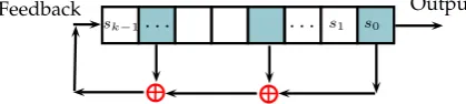
A common way to implement the generation of linear recurring sequences is to uselinear feedback shift registers(LFSR). LFSRs are useful tools both in coding theory and in cryptogra-phy. In particular they are one of the most useful devices in the generation of keystreams. A linear feedback shift register consists of two parts: a shift register of lengthkand a feedback

functionF. The shift register is a register with k cells each containing an element of_Fq. The

content of thekcells forms thestateof the LFSR. The feedback function is usually theXORof the content of certain cells, which are calledtaps. The first output sequence element is the least significant element of the initial state, i.e the element in the rightmost cell of the shift register. Then, the shift register is shifted by one cell to the right and the new leftmost cell is filled with theXOR of the taps. By iterating the previous procedure, the LFSR produces a semi-infinite sequence of elements inFq. Figure 2.2 shows a general LFSR in the Fibonacci representation.

Output Feedback

s0

s1

sk−1. . . .

Figure 2.2: Linear feedback shift register

In the following we recall some basic results concerning linear recurring sequences.

Definition 2.4.2.Let S be an arbitrary nonempty set, and lets0, s1, . . .be a sequence of elements

ofS. The sequences0, s1, . . .isperiodicif there exists an integerr >0such thatsn+r=snfor

Proposition 2.4.3. If s0, s1, . . . is a kth-order linear recurring sequence in a finite field Fq satisfying the linear recurrence relation(2.5), and if the coefficienta0 of (2.5)is nonzero, then

the sequences0, s1, . . .is periodic and its periodris≤qk.

Lets0, s1, . . .be an homogeneous linear recurring sequence inFq satisfying

si+k=ak−1si+k−1+ak−2si+k−2+· · ·+a1si+1+a0si for i= 0,1, . . . , (2.6)

whereaj ∈Fq, for0≤j ≤k−1. To this linear recurring sequence we associate the following

k_×kmatrix over_Fq

A=

       

0 0 0 . . . 0 a0

1 0 0 . . . 0 a1

0 1 0 . . . 0 a2

... ... ... ... ... ...

0 0 0 . . . 1 ak−1

       

. (2.7)

We note that the matrixAdepends only on the linear recurrence relation satisfied by the given

sequence. In particular it does not depend on the initial state of the sequence. The polynomial

f(x) =xk₋ak−1xk−1−ak−2xk−2− · · · −a0 ∈Fq[x]

is said thecharacteristic polynomial of the linear recurring sequence, and, as the matrixA, it

depends only on the linear recurrence relation (2.6). It is easy to see thatf(x) corresponds to

the characteristic polynomial of A in the sense of linear algebra. Linear recurring sequences

whose periods are very large are of particular interest in applications. Next Theorem suggests how to produce such sequences.

Theorem 2.4.4. Lets0, s1, . . .be an homogeneous linear recurring sequence inFqwith nonzero initial state, and suppose its characteristic polynomial f(x) _{∈ F}q is irreducible over Fq and satisfiesf(0)₆= 0. Then the sequence is periodic with period equal toord(f(x)).

By Theorem 2.4.4 it follows thatkth-order maximal period sequences in_Fqare those whose

characteristic polynomial is a primitive polynomial overFq, and its period is equal to the largest

possible value for the period of anykth-order linear recurring sequences in_Fq– namelyqk−1.

Sequences with maximal period have also many desirable statistical properties. The best known of these properties is to satisfy Golomb’s axioms for pseudo-random sequences [G+_82].

2.5

Discrete Logarithms

LetK =_FqandF =Fqm. UsuallyF is represented as anm-dimensional vector space over

K, so additions inF become trivial given the arithmetics inK. However, the choice of a basis

ofF over K is crucial for efficiently performing multiplication, inversion and exponentiation.

2.5. Discrete Logarithms

of bases of particular importance. The first is apolynomial basis_{1, α, α2_{, . . . , α}m−1_}whereα

is a root of an irreducible polynomial of degreemoverK. In this context, one often prefersα

to be a primitive element ofF. The second basis is anormal basis, that is, a basis of the form {α, αq_{, . . . , α}qm−1_}.

An alternative to using basis representations is to represent the non-zero elements ofF as the

powers of a primitive elementα _∈F. In this case multiplication inF is trivial, but addition then

becomes difficult. In practical applications where repeated computations over a relatively small finite field are required, this problem can be overcome using discrete logarithms in conjunction with Zech logarithms. In addition to this employment, discrete logarithms in finite fields play an important rule in cryptanalysis.

In this subsection we summarize the main current algorithms for computing discrete loga-rithms in finite fields and their use to improve arithmetic in small finite fields.

Definition 2.5.1(Discrete Logarithm). Letα_{∈ F}qa primitive element andβ ∈Fq, β 6= 0. We

define the discrete logarithm ofβ with respect toα as the unique integer0 _≤ i < q such that αi =β. We use the notationi= DLog_α(β).

2.5.1 Computing Discrete Logarithms

The most obvious method for finding discrete logarithms inFq is to precompute a table of

logarithms once and for all time. Another one is to successively compute consecutive powers of

αand compare withβuntil a match is found. Both methods become computationally infeasible

whenqis sufficiently large, since they costO(q). A more interesting method, but still not very

practical, to compute discrete logarithms inFq withq = ps is given by Mullen and White in

[MW86] and it consists in exhibiting a polynomial representation for theDLogfunction modulo

p. They prove the following result

Proposition 2.5.2. Letαbe a generator for_Fq withq = ps_{. For anyβ =α}i _∈

F∗q,q ≥ 3, we have that

i_{≡ −}1 + q−2

X

k=1

βk

α−k₋₁ (mod p)

The two main kind of methods used to compute discrete logarithms in finite fields are the Pohlig-Hellman methodcombined with theBaby-step Giant-step algorithmor with the

Pollard-ρalgorithm, and theIndex-Calculus method. In practice, many computational algebra systems use the Pohlig-Hellman method for computing discrete logarithms in Fq when the maximal

prime factor of q is approximately less than 236, and they use Index-Calculus method in the

other cases.

Baby-step Giant-step algorithm

The first algorithm we describe is the Baby-step Giant-step algorithm attributed to Shanks. The algorithm works as follows. Letr, sbe integers withr_·s > q. Precompute a list of pairs,

(i, αi_{)for0 ≤i < r and sort this list by second component. These precomputations are called} baby-steps. The giant steps consist on computing for eachj, 0 _≤ j < s, the element βα−jr

and see (by a binary search) if this element is the second component of some pair in the list. If

βα−jr =αi for somei,0 _≤ i < r, thenDLog_α(β) = qifi =j = 0 andDLog_α(β) = i+jr

otherwise. The baby steps require a table withO(r)entries, while to sort the table and search the

table for each value ofjrequiresO(r+s)field operations. Usually one chooser =s =√q₋1

in order to getO(√q₋1)for both time and memory complexity.

Pollard-ρmethod

One drawback of Shanks algorithm is the need to sort and store a list of size √q₋1.

Pol-lard [Pol78] introduced a probabilistic algorithm which eliminates the need for such storage. PartitionF∗q into three setsS1, S2, S3 of roughly equal size. Consider the sequence of elements

inF∗q x0, x1, x2, . . .withx0 = 1and

xi =

      

βxi−1 xi−1 ∈S1

x2

i−1 xi−1 ∈S2

αxi−1 xi−1 ∈S3

It is easy to see that this sequence defines two sequences of integers{ai}and{bi}wherexi =

βai_αbi, _i≥₀,_a

0 =b0 = 0,ai+1 ≡ ai+ 1,2aiorai (mod q−1)andbi+1 ≡bi,2bi orbi+ 1 (mod q₋1)depending on which setS1, S2orS3 containsxi−1. Making use of Floyd’s cyclic

algorithm, Pollard computes the six-tuple(xi, ai, bi, x2i, a2i, b2i)untilxi =x2i. At this stage we

haveβr _=αs_{withr ≡a}

i−a2iands≡bi−b2i (mod q−1). It follows thatrDLogα(β)≡s (mod q₋1). Since there are onlyd= GCD(r, q₋1)possible values forDLog_αβ, ifdis small

then each of these possibilities can be list to obtain the correct value.

Making the heuristic assumption that the sequence {xi}is a random sequence in F∗q, then

the expected time complexity of this method isO(√q₋1)field operations.

Pohlig-Hellman method

The Pohlig-Hellman method computes discrete logarithms in finite fields taking advantage of the integer factorization ofq₋1. Letq₋1 =Qt

i=1p

ei

i wherepiis a prime number andeiis a

positive integer, for1_≤i_≤t. Ifx= DLog_α(β)then the approach of Pohlig and Hellman is to

obtainxmodulopei

i for eachiand then use the Chinese Remainder Theorem to getx modulo

2.5. Discrete Logarithms

e a positive integer. Lete0 = de/2e and e1 = be/2c. We have that x = x0 +pe0x1, where

0_≤x0 < pe0 and0≤x1 < pe1. Soβ =αx =αx0+p

e0_x1

. Elevating both sides tope1 we get

βpe1

=αpe1x0+pe0pe1x1 _=αpe1x0+pex1 _=αpe1x0_,

where the last equality holds becauseαis a primitive element in_Fq. Thenx0 = DLogp

e₁

α (βp

e₁

).

Sinceβα−x0 _=αpe0x1, then_x

1 = DLogp

e₀

α (βα−x0). Using one of the two previous methods we

determinex0andx1, and thusx.

For the case where q₋ 1 = pe _{this technique requires O(e(log(q− 1) +}p

(p) log(p)))

[PH78].

Then, using Pohlig-Hellman algorithm in conjunction with Baby-step Giant-step method or with Pollard-ρmethod one can compute discrete logarithms in_Fqin approximatelyO(

√

I)field

operations, whereI is the largest prime dividingq₋1. Note that in this case the characteristic

p of the field is irrelevant. Basing on the computationally capacity of modern computers is

reasonable to use this method whenIis relatively small, say less than236. As a consequence, if

one is going to design a cryptographic system based on a finite fieldFq one must selectqsuch

that the factorization ofq₋1contains a suitable large prime.

Index Calculus

Unlike the Shanks and Pollard-ρmethods, which take exponential time (O(√q₋1)field

op-erations), index calculus techniques are subexponential with heuristic running timeL[q,1/3, c],

and evenL[q,1/4, c]in some cases. The basic idea of index calculus algorithms dates back in

1922 in the work of Kraitchik [Kra22, pp.119-123].

LetFq be the finite field in which we want to compute the discrete logarithm and letα be

a primitive element ofFq. Consider a subset S ={p1, p2, . . . , pt}ofFq with the property that

a ”significant “ fraction of all elements inFqcan be written as the product of elements fromS.

The setS is usually called thefactor base for the index calculus method. The index calculus method consists of two main stages. In the first stage one attempts to find the discrete logarithms of all the elements ofS. In the second stage one compute logarithms of elements in_Fq which

are not inS. To obtain discrete logarithms of elements ofS we proceed as follows. We pick a

random integeraand attempt to writeαa_{as a product of elements inS, α}a ₌ Qt i=1p

λi

i . If we

are successful then we have that

a_≡XλiDLogαpi (mod q−1).

After collecting a sufficient number, i.e greater thant, of relations of this type, the corresponding

system of equations can be expected to have a unique solution for the variables DLog_αpi, 1_≤ i _≤ t. Letβ _{∈ F}∗_q. To computeDLog_αβ we repeatedly pick an integersat random until αsβ can be written as the product of elements inS, that isαsβ = Pt

i=1p

bi

we have that

DLog_αβ _≡

t

X

i=1

biDLogαpi−s (mod q−1).

Note that to complete the description of the method one should precise how to choose the set S and how to efficiently generate the relations expressing an element of_Fq as product of

elements inS.

In the last fifty years several different index calculus algorithms were developed forFqwith

q = pn_{, and the best algorithms vary with the relative sizes of the characteristic p and the}

extension degreen.

For a long time the best index calculus algorithms for discrete logs had running times of the formL[q,1/2, c]for various constantsc >0. The first practical method that broke through

this running time barrier was Coppersmith’s algorithm [Cop84] for discrete logs in fields of size q = pn where p is a small prime and n is large. It had running time of approximately L[q,1/3, c] with c varying slightly with the values of p and n. This initial progress quickly

led to the introduction of several other heuristic algorithms with similar running time. For a long time, index calculus algorithms focused on field with small characteristic, prime fields and occasionally fields of the formFpn for small values ofn [Sch00]. The view changed in 2006, when was showed that taken together, the Number Field Sieve [JL06] and the Function Field Sieve [AH99] are enough to cover the whole range of finite fields. Both these algorithms have heuristic running time ofL[q,1/3, c]. Essentially, the consequence was to split the finite field in

three groups, small characteristic with complexityL[q,1/3,(32/9)1/3], medium characteristic

with complexityL[1/3,(128/9)1/3_{]and large characteristic with complexityL(1/3,(64/9)}1/3_).

In 2013 and 2014, two notable improvements on the complexity of discrete logarithm algo-rithms have been made: two variants of the Number Field Sieve have been designed for finite fields with medium to high characteristic [BP14] and the complexity for finite fields with small characteristic have been dropped to approximatelyL[q,1/4, c][Jou14, BGJT14, GKZ14]].

We conclude this subsection by noting that the expected running times of all the previous algorithms are heuristic, and that the best algorithms with rigorously proved expected running time cost approximatelyL[p,1/2,√2][MBG+_13].

2.5.2 Zech Logarithm Table

In small finite fields is useful to employ tables of Zech logarithms to efficiently perform additions and multiplications. The procedure is the following.

LetFq be a finite field. Represent the non-zero elements ofFq as the powers of a primitive

elementα _{∈ F}q. Then, identifying the elements of Fq with their discrete logarithms, the

mul-tiplication of two elements in Fq is reduced to the addition of the corresponding two discrete

logarithms, since

2.5. Discrete Logarithms

where the addition is modulo q ₋1. In this representation, to perform the addition of two

elementsβ, γ _∈Fqone needs to compute the discrete logarithmDLogα(β+γ). Sinceαa+αb =

αa(1 +αb−a), to do that it suffices to compute the discrete logarithms for sums involving1, i.e.

logarithms of the formDLog_α(1 +γ). This motivates the following definition

Definition 2.5.3(Zech’s Logarithm). Let_Fqbe a finite field and letαbe a primitive element of

Fq. TheZech’s logarithm(orJacobi logarithm) with baseαof an integernis the integerZα(n)

defined by the equation

1 +αn =αZα(n)_,

where the caseαn_{=−1is excluded.}

When q is small, say less than 220, the Zech logarithms can be precomputed and, when

needed for an addition, recovered by a simple table lookup. Moreover, exploiting some prop-erties of Zech’s logarithm [Hub90] one can reduce the storage requirements fromq = pk _to

roughlyq/6k.

Decoding Problem for Cyclic Codes

The main problem of information theory can be described as follows. Suppose that a source of data has been transmitted over a noisy channel. In this context, the following question arise naturally: how can we tell when the original data has been changed? And when it has, how can we recover the original data? One of the goal of Coding Theory is to answer to the two previous questions.

In the first section of this chapter we formalize the above problems and introduce error correcting codes. In Section 3.2 we recall some basic properties of linear codes and discuss the complexity of decoding problem for these codes. Finally, in Section 3.3, after recalling some properties of cyclic codes, we address the decoding problem for cyclic codes and discuss interesting open problems regarding general error locators.

Most of the results in this chapter are well-known in the literature. Here we use as main references [MS77], [PW72] and [PHB98].

3.1

An overview on error correcting codes

Coding theory is the study of the properties of codes and their suitability for a specific application. One of these applications is the design of efficient and reliable data transmission methods. A code designed with this purpose is called anerror correcting code. There are two fundamentally different types of codes: block codeswhich break the sequence of information digits intok-symbol blocks, andtree codeswhich operates on the information sequence without breaking it into independent blocks.

In this thesis attention is focused on block codes. From now on, when we say error correct-ing codes we actually mean block error correctcorrect-ing codes.

Definition 3.1.1. Let_Fq be a finite field. A subsetC ofFqnof sizeM is called ablock code(or

also aq-ary block code) of lengthnand sizeM over_Fq, and its elements are calledcodewords.

We call an element ofFqasymbol, and an element ofFqn(which is not necessary inC) aword.

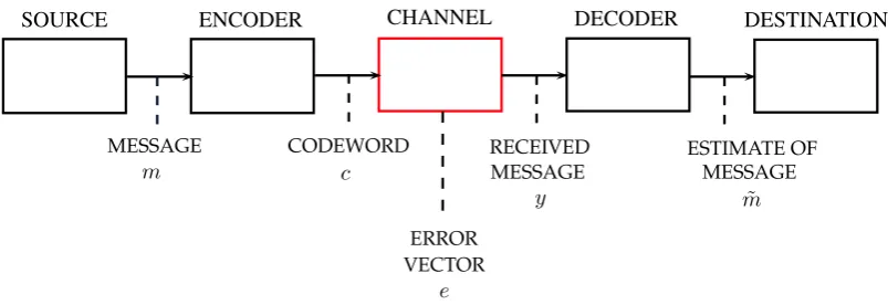
A general communication system which uses an error correcting codeCis showed in Figure

3.1. It consists of essentially five parts:

1. Aninformation source: which produces a messagem = (m1, . . . , mk) ∈ Fqkto be

DESTINATION

SOURCE ENCODER CHANNEL DECODER

MESSAGE CODEWORD RECEIVED ESTIMATE OF MESSAGE MESSAGE

ERROR

m c

e

y m˜

VECTOR

Figure 3.1: A simple model of communication system. We omit to represent both the transmitter and the receiver.

2. An encoder: which produces a codeword c = (c1, . . . , cn) ∈ C,where n > k, from a

messagem

3. Atransmitter: which operates on the codewordcin order to produce a signal suitable for

transmission over the channel

4. Anoise channel: which is the medium used to transmit the signal from a transmitter to a receiver, and it is supposed to be noisy

5. Areceiver: performing the inverse operation of the transmitter, i.e. recovering the word

y_∈Fn

q corresponding to the received signal

6. Adecoder: which tries to recover the original messagemfromy

7. Adestination: the person who the message is addressed to.

We callencodingthe process of converting the messagem _∈Fk

q into a codewordcof a given

codeC. The process of recovering the messagesmfrom the received wordyis saiddecoding. The central idea in using error-correcting codes for communication data is that the sender encodes the message in a redundant way by using an error-correcting code in a such way (de-pending on the channel used for the transmission) that the redundancy allows the receiver to detect and/or correct possible transmission errors.

Example 3.1.2. Let us consider the set

C =_{00000,01011,10101,11110_}.

C is a binary code of lengthn= 5withM = 4codewords.

Suppose that we want to employ C in order to guarantee a reliable transmission data over a

noisy channel, and that the (corrupted) codewordy = 00101is received. The set of possible

3.1. An overview on error correcting codes

From the previous example it is clear that to decide which error out of a set of errors is the “right one”, that is to decode, one needs to make additional assumptions about the likelihood of errors and error patterns. One need also to specify how the sent codewordscand the error

patternseare combined to form the received codewordsy=f(c, e).

Throughout all the thesis we will assume that for aq-ary code, codewordscand error patterns eare combined through a moduloq addition, that isy = c+e where+is the addition in_Fqn.

A such channel is called anaddition channel. We will also assume that the channel is an q-ary

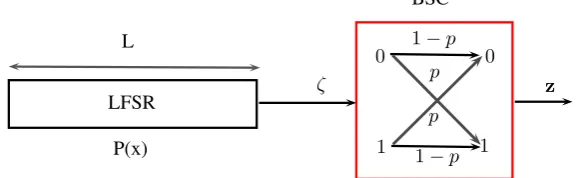
symmetric channel. In the next definition we recall the notion of symmetric channel.

Definition 3.1.3(q-ary symmetric channel). Aq-ary symmetric channel(qSC)without memory is a discrete channel withq-ary symbols both as inputs and as outputs. Moreover it satisfies the

following properties

• the probability that a symbol changes into another is the same for all theq₋1symbols

• the probability that a symbol changes does not depend on its position in the transmitted word

• if the ith component of a transmitted word changes, then this fact does not affect the

probability that itsjth component changes

The transition probabilities of theq-ary symmetric channel depend on a single parameter

as follows

P[b|a] =

  

1₋ b=a

/(q₋1) b₆=a

whereP[b|a]denotes the probability to receive the symbolb given that the symbolawas sent. In other words, in aq-ary symmetric channel every symbol is left untouched with probability

1₋and is distorted to each of theq₋1possible different symbols with probability.

An important requirement in order to define a transmission model is to fix a distance measure between codewords. The most prevalent measure for our purpose is Hamming distance, which is defined as follows.

Definition 3.1.4. Given two vectors x = (x0, . . . , xn−1) and y = (y0, . . . , yn−1) in Fqn, we

define the Hamming distance between x and y as the number of components in which they

differ

d(x, y) = _|{0_≤i_≤n₋1_|xi 6=yi}|.

TheHamming weight of a vectorx _∈Fn

q is the number,w(x), of its non-zero components, i.e. w(x) = d(x,0).

LetC be aq-ary code,y _{∈ F}n

q be the received word, andebe the error vector occurred in

Definition 3.1.5. We say thatC has error correction capabilityt (or thatC can correct up to terrors) if for any error vector ewithw(e)_≤ t, Callows to recoverx. Similarly, we say that C haserror detection capabilitys(or thatC can detect up toserrors) if for any error vectore

withw(e)_≤s,Callows to detect that an error occurred in the transmission.

Next two definitions introduce two important parameters of an error correcting code.

Definition 3.1.6. TherateRof aq-ary block code of lengthnwithM codewords is given by

R = (log_qM)/n

The rate of a code is a measure of the efficiency of the code.

Definition 3.1.7. The redundancy r of a q-ary block code of length n with M codewords is

given by

r =n₋log_qM.

We can say that the birth of the subject of coding theory for data transmission occurred in 1948 when Shannon published the paper “ A Mathematical Theory of Communication” [Sha48]. His work focuses on the problem of how best to encode the information a sender wants to transmit. He established the limits of the gains possible with coding theory, and proved the existence of codes that could effectively reach these limits. More precisely, Shannon showed the following theorem. Beforing stating it, we introduce the capacity of aq-ary symmetric channel.

Definition 3.1.8. Given aq-ary symmetric channel with probability of symbol error, we say

that the capacity of the channel is

C() = 1 +log_q() + (1₋) log_q(1₋)₋plog_q(q₋1).

Theorem 3.1.9(Shannon). For any δ > 0andR < C(), there is a (linear) code over_Fq of rateR0 _≥RwithPerr < δ, wherePerris the probability that the output of the decoder does not correspond to the originally transmitted vector.

So, if one wishes to communicate over a channel of capacity Q at a rate R, then one can do

so as reliably as desired, if and only if R < Q. Although Shannon [Sha48] answered to the

question “Do good codes exist?” affirmatively, his work raises two other questions “ How can we construct such codes?” and “How can we decode them?”. In a sense, the study of error correction codes is all about these two questions.

3.2

Linear Codes

3.2.1 Basic definitions

3.2. Linear Codes

Definition 3.2.1. LetC be aq-ary block code of length n. We say thatC is a linear (block)

code if it is a linear subspace of the vector spaceFqn. If the dimension of the subspaceC isk,

then we say that the codeChasdimensionkand thatCis a[n, k]-code.

We do not treat in this thesis the case of non-linear block codes, so often we will use the word “code” for referring to linear block code. When we do not specify the field, we implicitly mean that the code is defined overFq. Note that if C is an[n, k]-code over Fq, then|C| = qk

where|C_|denotes the cardinality ofC.

As subspace ofFqn, an[n, k]-code admits a basis. This leads to the definition of a generator

matrix of a code.

Definition 3.2.2. LetC be an[n, k]-code over_Fq. Any matrixGwhose rows form a basis for

Cas ak-dimensional subspace of_Fqnis called a generator matrix ofC.

IfGhas the formG= [1k|A], where1kis thek×kidentity matrix, thenGis called a generator

matrixin standard form. In general, there are many generator matrices for a codes, nevertheless any code has a unique generator matrix in standard form.

Given x = (x0, . . . , xn−1) and y = (y0, . . . , yn−1) in Fqn, we denote by x· y the scalar

product ofxandyin_Fn

q, that isx·y=

Pn−1

i=0 xiyi. We recall thatxandyare saidorthogonal

ifx_·y= 0.

Definition 3.2.3. LetCbe an[n, k]-code. The setC⊥of vectors in_Fqnwhich are orthogonal to

all codewords ofCis again a linear code and it is called thedual codeofC.

We note that the dual code of an[n, k]-codeCis an[n, n₋k]-code.

Definition 3.2.4. Aparity-check matrixHfor an[n, k]-code is a generator matrix ofC⊥.

By previous definitions we easily get that ifC is an[n, k]-code then a generator matrixG

ofChas sizek_×nand a parity-check matrixH has size(n₋k)_×n. To check if ann-vector x_∈Fn

q belongs toCit is sufficient to computeHxT. Indeed it holds that

∀x_∈Fqn, HxT = 0 _←→x_∈C (3.1)

Definition 3.2.5. LetCbe an[n, k]-code over_Fql. Thesubfield subcodeC

FqofCwith respect

toFqis the set of codewords inCeach of whose components is inFq.

BecauseCis linear over_Fql, thenC

Fqis a linear code overFq.

Remark3.2.6. LetC be an[n, k]-code over _Fql andH be a parity-check matrix ofC. To find a parity check matrix forC_Fqconsidering a basis_{b1, b2, . . . , bl} ⊂ Fql of_Fql over_Fq. Each elementz _∈Fqlcan be uniquely written asz =z₁b₁+· · ·+z_lb_l, wherez_i ∈_Fq for1≤i≤l. Associate toz the column vectorz¯= (z1, . . . , zl)T. CreateH¯ fromH by replacing each entry

hby the vector¯h. BecauseH is an(n₋k)_×nmatrix with entries in_Fql,H¯ is al(n−k)×n matrix overFq. A parity check matrix forC_Fqis obtained fromH¯ by deleting dependent rows.

Definition 3.2.7. The minimum distance (or simply the distance) of a codeC is the smallest

(Hamming) distance between distinct codewords, that is

d(C) = min_{d(x, y)_|x, y _∈C, x₆=y_}.

IfCis a[n, k]-code and we known the distance ofCthen we also refer to it as an[n, k, d(C)]

-code.

The following result shows that it is possible to define the distance of a linear code using the weight of codewords instead of mutual distance between all codewords.

Proposition 3.2.8. LetCbe an[n, k, d]-code. Thend(C) = min_{w(c)_|c_∈C, c₆= 0_}.

LetCbe an[n, k, d]linear code over_Fq. IfDis a vector subspace ofC, then we say thatD

is a (linear) subcode ofC. Moreover we haved(C)_≤d(D).

Definition 3.2.9. LetC be an[n, k, d]-code. We denote byAi the number of the codewords of

weighti. The set of_{Ai}0≤i≤nis called the weight distribution ofC.

Definition 3.2.10. LetC1 andC2 be two linear codes. We say thatC1 andC2 arepermutation

equivalentif there is a permutation of coordinates which sendsC1 toC2.

Two permutation equivalent codes have the same weight distribution.

Proposition 3.2.11. Let C be linear code and let H be a parity-check matrix ofC. Then C

has distancedif and only ifH has a set ofdlinearly dependent columns and any set ofd₋1 columns is linearly independent.

The following theorem is a consequence of the previous result. It gives an upper bound for the distance of a code.

Theorem 3.2.12(Singleton bound). LetCbe an[n, k, d]-code. Then

d _≤n₋k+ 1

A code reaching the equality in the Singleton bound is called a maximum distance separable codeor anMDScode.

Definition 3.2.13. Let xbe any vector in _Fn

q and letC be an[n, k, d] code with parity-check

matrixH. The vectors _∈ (_Fq)n−k such thats = HxT is called the syndrome vector of xwith respect toH (or simply thesyndrome of x).

Equation (3.1) tell us that a vectorx_∈Fqnis a codeword ofCif and only if the syndrome of xis zero. The syndrome, however, tell us more than a vector being in the code or not. Suppose

the vectorcwas transmitted andv was received, wherev =c+e, withethe error vector. Note

that

s=HvT =H(c+e)T =HcT +HeT =HeT,

sincec_∈C. Then, the syndrome does not depend on the received vector but on the error vector.

3.2. Linear Codes

Proposition 3.2.14. LetC be an[n, k, d]-code and letH be a parity-check matrix ofC. Then, there is a1-1correspondence between errors of weight_{≤ b}(d₋1)/2_cand syndromes.

This property of linear codes justify the following definition

Definition 3.2.15. LetC be an[n, k, d]-code over_Fq. We callcorrectable syndromesthe

syn-drome vectorss_∈Fn−k

q corresponding to errors of weightµ≤twitht=b(d−1)/2c.

Proposition 3.2.16. LetCbe an[n, k, d]-code over_Fq. Then

• C has detection capabilityd₋1

• C has error correction capabilityt=_bd₋1_c/2.

The previous result shows that the distance of a code reflects the error correction capability of the code. Evidently, we would liket, and hence alsod, to be large.

We conclude this section summarizing the properties a good error correcting code should have. In the study of error correcting codes it is important to construct[n, k, d]-codes having

the following properties:

1. large rateR;

2. large distanced;

3. admitting efficient encoding and decoding algorithms.

There is a trade-off between the rateRand the minimum distancedfor any linear code. Indeed,

by the Singleton bound and the definition of rate of a code, we have that

R+ d

n ≤1 +

1

n.

So we have to make a compromise between the rate and the minimum distance. The third property above is also very important for a code, as codes with large rate and distance may be useless if they have no efficient encoding and decoding algorithms. In the next section we trait the problem of decoding linear codes.

3.2.2 Decoding Linear Codes

Suppose to use an [n, k]-code C over _Fq for a reliable transmission of data over a noisy

channel, and to receive the wordy_∈Fn

q. The optimal decoding strategy is to find the codeword

c_∈C that maximizes the probabilityP r(c_|y)thatcwas transmitted given thatywas received.

On a q-ary symmetric channel, this strategy is equivalent to find the closest codeword toy in

the Hamming metric [MS77].

Definition 3.2.17. A decoder forC that always finds the closest codeword tor(or one of the

Maximum-likelihood decoding of aq-ary[n, k, d]-code can be trivially accomplished inO(qk₎

by simply computing the Hamming distance between the received wordy and all theqk

code-word of C. However, this procedure is computationally infeasible when the number of

code-words is large. An other method accomplishing this task is the following, which costsO(qn−k_).

LetC be an[n, k]-code over_Fq. For any vectoru∈Fnq the set

u+C=_{u+c_|c_∈C_}

is called a coset of C. Every vector of _Fn

q is contained in such a coset. Since C is a linear

subspace ofFqn, two cosets are either disjoint or identical. Suppose that a codewordxwas sent

via a noisy channel, and a vectoryis received, then the error vector ise=y₋x. LetH denote

a parity check matrix ofC. It follows thatHeT _=HyT_{, that is the syndrome ofecorresponds}

to the syndrome of y. Obviously, all the vectors of a coset have the same syndrome. The

minimum weight vector of a coset is called the coset leader (if there is more than one vector with the same minimum weight, choose one at random and take it as the coset leader). A naive decoding procedure consists in first computing the syndrome of a received vector HyT, then

take the coset leadereof the coset having syndromeHyT _{as the error vector, and finally decode}

the received vectoryto bey₋e. Since the number of possible syndromes isqn−k_{, this method}

costsO(qn−k).

Although maximum-likelihood decoding is the optimal decoding strategy, Berlakamp et al. [BMvT78] showed that for the general class of linear codes, polynomial-time maximum-likelihood decoding algorithms are unlikely to exist (unless P=NP). Bruck and Naor [BN90] showed that this remains true even if the code is known in advance and can be preprocessed for a long as desired in order to devise a decoding algorithm. Moreover, such algorithms are not known today even for any specific family of useful codes, such as the binary BCH codes, for instance. On the contrary, in [GV05], it was proved the NP-completeness of maximum likelihood decoding for generalized Reed-Solomon codes. A potential way