The numerical inversion of Abel type integral equations in stereology

THE NUMERICAL INVERSION OF

ABEL TYPE INTEGRAL EQUATIONS IN STEREOLOGY

by

Anthony J. Jakeman

A thesis submitted to the Australian National University for the degree of Doctor of Philosophy

TABLE OF CONTE

N

TS

ACKNOWLEDGEMENTS PREFACE

(i ) (ii) ( iii) ABSTRACT

CHAPTER 1: Introduction 1.1 Introduction

1.2 Stereology and Abel type integral equations 1.3 General comments on the inversions

1.4 Thesis outline

CHAPTER 2: Mathematical Models in Stereology: the Abel Type Equation and the Numerical Differentiation Problem

2.1 Introduction

2.2 Preliminaries and notation

2.3 The Santalo formulations for convex particles CHAPTER 3: Numerical Procedures for Integral Equations of Abel Type

3.1 Introduction

3.2 Basic properties of integral equations of Abel type and the stereological data

3,3 Numerical methods for Abel type equations in stereology

l 2 3 5

8 9 10

15

17

24

3,4 Spectral differentiation 35

3.5 Product integration 38

3. 6 Evaluation of inversion formulas 41 3,7 Statistical and numerical properties of Procedure (II) 45 3.8 Reliability of the random spheres approximation 47

3,9 Conclusion 52

CHAPTER 4: An Inversion of a Singular Second Kind Volterra Equation: The Thin Section Equation of Stereology

4 .1 Introduction 51~

CHAPTER 5: Product Integration for Estimating Functionals of Particle Size Distributions

5.1 Introduction 74

5.2 Consistency and variance properties of the estimates 77 5.3 Estimation from truncated empirical data 85

5.4 Numerical results 88

CHAPTER 6: Inversion of a Class of First and Second Kind Convolution Volterra Equations

REFERENCES

6.1 Introduction

6.2 Inversion formulas, and existence and uniqueness of solutions

93

99 6.3 Determination of the kernels in the inversion formulas 107 6.4 Evaluation of inversion formulas 112 6.5 Other problems with inversion formulas 115

6.6 Conclusion 116

ACKNOWLEDGEME

N

T

S

The work for this thesis was undertaken at the Computer Centre, Australian National University, with the financial assistance of a Commonwealth Postgraduate Research Award. I thank Mike Osborne for his general support as director of the centre.

( i)

Particularly I thank Bob Anderssen whose enthusiasm for research I best describe as admirable and contagious. His suggestions concerning the

line of research, his stimulating supervision and advice about the

presentation of the thesis are highly appreciated. Thanks also go to Peter Bloomfield. His discussions with Bob and myself which led to the

crystallisation of Chapter 5 were very rewarding. Thanks are also due to Roger Miles whose interest in the work was encouraging and whose advice and support were most helpful,

Kind thanks are due to Mrs Barbara Geary for her high-standard typing as well as to my contemporary, Bernard Omodei, for his careful checking of the final typescript.

(ii)

PREFACE

Much of the work in this thesis was carried out in collaboration with R.S. Anderssen. In particular, Chapters 3, 4 and 5 are based on results established jointly.

The publication details of the thesis are Jakeman (1975), Jakeman and Anderssen (1974, 1975a, b) and Anderssen and Jakeman (1974, 1975a, b, c). Often the text of these papers has been closely followed.

(iii)

ABSTRACT

Abel type integral equations of the form

I

00 k / t )k2 (s)

h(t) = - - - - g(s)ds , t (s-t)a.

0 <a.< 1, s ~ t ~ 0 ,

arise frequently in stereology. This thesis mainly examines the evaluation of the corresponding inversion formulas

g(t) + Icx,t 1

(s-t/-a.

d {h(s)

}ds]

&9sT

( :'.:':)

given non-exact empirical data. The evaluation is stabilised by the use of product integration to approximate the singular integral terms, and spectral differentiation to determine the numerical derivatives. Extension of the inversion techniques to other types of problems is also considered.

After an introductory discussion of stereology and the more specific equations under consideration in this thesis in Chapter 1, Chapter 2

demonstrates the relevance to stereology of the Abel type integral equation and the numerical differentiation problem.

Chapter 3 presents methods for the numerical inversion of(*) via the evaluation of ( M:). Consistency and order of convergence results are given. Particular attention is paid to the random spheres equation as well as to the reliability of the random spheres approximation. It is concluded from the results that the approximation is robust for near-spherical particles.

In Chapter 4, an inversion method is developed for the thin section equation of stereology, which is a singular second kind Volterra equation with a convolution kernel.

The method of evaluation of the integral terms in these inversion

(iv)

functionals , which are satisfactory in the sense of efficiency, consistency and finite variance, have previously failed. Solutions to this problem using the technique of product integration are presented in Chapter 5.

The types of integral equations for which the inversion methods of Chapters 3 and 4 can be applied are extended in Chapter 6 to a large class of convolution Volterra equations of the first and second kind. Again the methods are particularly applicable when the data provided are non-exact. Even when an inversion formula is not known analytically, it is shown that under general conditions there still exist inversion methods based upon Laplace transformations. When compared with integral equations which possess explicit analytic inversion formulas, the extra computational work

l

CHAPTER 1

INTRODUCTION

1.1

Introduction

The generalized Abel integral equation

h(t) = It k(t,s~ g(s)ds o ( t-s)

o

<a< 1,

o

st s

T < oo

'

(l.l.l)

where k(t, s) is continuous on OS s St ST and k(t, t)

t

O , is of considerable importance in many fields.

Consider the particular case when k(t, s) is separable in (1.1.l) and the range of integration is (t, 00 ) :

f

oo k

1(t)k2(s)

h(t) = - - - - g(s)ds

t

(s-tf

o

< a< 1, s ~ t ~

o

.

(l.1.2)

It is these Abel type equations which occur frequently in stereology and to which we shall confine attention. Furthermore, when g(t)k

2(t) is

continuous , k

2(t)

t

O and h(t)/k1(t) is differentiable, (1.1.2) can be easily shown to possess the following inversion formulas:

g(t) = -[1rk2(t)]-\in(a1r)[ h(s) 1-al k

1 (s)(s-t) s~

+ ( (s-t~l-a

-1:,

{~:(;1}

as]

(1.1.,1

= -[1rk

2(t)]-\in(a1T)

-#z/; (

1

_!:18b

ds (l.1.4)

m;; (s-t/-a 1<_{1 ~s,}

In this thesis, numerical schemes for (1.1.2) based upon the evaluation of (1.1,3) and (1.1.4), given non-exact stereological data, are mainly

2

integral equations with aonvolution kernel k , viz.

Ag(t) = h(t) +

J

:

k(t-s)g(s)ds t ~ 0 • (1.1.5)

If

A

t

O , (1.1.5) is said to be of the second kind and is of the fir·st

kind otherwise.

When A= l , this is the well-known renewal equation which has

importance in the theory of stochastic processes, queuing theory and inventory

theory. It is also of practical interest in meteorology, engineering and

physics. The first kind equation is a fundamental relation in system

analysis. Bellman et al. (1966) provide further details and references

regarding the applications of (1.1.5).

1.2 Stereology and Abel Type Integral Equations

Stereology involves the estimation of three-dimensional structure from

observations in lower dimensions (see Moran (1972) for a broad review of the

subject). Deduction of structure of a particulate phase, for instance, may

involve estimation of any or all of the following properties of that phase:

shape, number, volume, size, surface area and length. When simple logic

fails, mathematical methods based on geometric probability, statistics and

numerical analysis are required to formulate and solve the equation relevant

to the model used.

For example, Santalo (1955) considered the case of size estimation of a

particulate convex phase of similar shape, randomly distributed in a convex

field. The formulations produced fall essentially into three categories

defined by the nature of the lower-dimensional data. These data comprise:

(a) intersections of convex particles or flat convex particles

on random plane sections taken through an opaque field,

(b) p~ojections of line segments or flat convex particles on

random planes taken through a transparent field,

taken through an opaque field.

As will be seen in Chapter 2, quite often the model yields an equation

of Abel type. The most widely known and used example is the random spheres

equation

3

h(y) = 'fl... [ g(x) dx

m _y ( _X

2

_-y

2)¥

(l.2.1)

where

m =

I:

xg(x)dx .

However, one important exception, which is discussed in Chapter 4, does

arise. It is the thin section equation

I

oo s(x)dx

(2a+T)c(y) = 2y _{2 2} k + Ts(y) y

(x

-y ) 2

x ~ y ~ O . (l.2.2)

This second kind Volterra integral equation has wide use, particularly in

transmission microscopy.

For the stereological formulations which arise in this thesis, certain

minimum conditions are required for the equations to be valid. The convex

particulate phase must be homogeneously and isotropically distributed. As

well, the sample must possess ergodicity; that is, the sample distribution

function must approach a limiting distribution (see Miles ( 1975, pp. 217-218)

for a discussion of these three properties). One way of satisfying these

conditions is to constrain the convex particles to be randomly dispersed and

their centres to be located by a Poisson process of sufficiently low

intensity.

1.3 General Comments on the Inversions

The methods proposed here for the solution of the equations (1.1.2),

( l. l. 5) and ( l. 2. 2) are based on the evaluation of their inversion formulas.

Whether they be analytically explicit or not, the formulas always involve

4

an appropriate quadrature rule and spectral differentiation, respectively. In order that such schemes be stable and efficient, it is first

necessary to ensure that the quadrature rules used yield good approximations

to the integral terms involved, Thus, special care must be taken when

dealing with inversion formulas where a singularity occurs in the integrand. In this case, product integration methods have been found particularly

suitable. The product integration technique was first applied by Young

(1954) to integral equations and has since received considerable attention

in this context by Noble (1964), Atkinson (1967), Linz (1967), Hung (1970), Weiss and Anderssen (1972), Weiss (1972b), de Hoag and Weiss (1972),

Anderssen, de Hoag and Weiss (1973), Anderssen and Jakeman (1974), Jakeman and Anderssen (1974), Atkinson (1974), Anderssen and Jakeman (1975a, b) and

Anderssen (1975),

With regard to this question of stability and efficiency, it is also

necessary that the data

{vk}

for the spectral differentiation satisfy (see

Anderssen and Bloomfield (1971_{!a, b)) the following conditions:}

{l,3.1) the grid

{yk}

on which

{vk}

is defined must be uniform,

(l,3,2)

{vk}

must have a representation

vk

=

u(yk)

+

Ek

for all

k

,

where the continuous signal

u(y)

and the noise have

been generated by independent stationary stochastic processes

with mean zero, and

(1,3,3) the number of data points must be large enough so that an accurate spectrum analysis of

{vk}

can be made.

Most numerical schemes for solving (l.1.2), (l .1.5) and (l.2.2) previously involved the discretization of the equations at a number of

distinct points and the subsequent application of quadrature rules to

approximate the integral terms. Such schemes almost invariably provide for

the case of exact data only. For example, consider the first kind Volterra equation

5

h(t ) =

I

:

k(t, s)g(s)ds • (l.3.1) Becuase this is an improperly posed problem, small perturbations in h may

cause large perturbations in the solution g _{The effect of this in the}

numerical schemes considered by Weiss (1972a) is that for a uniform grid

width 6 , a perturbation

ohl

in

h

results in a perturbation in

g

of

ogl

which is proportional to

ohl/6

Thus, for non-exact data, there exists a dilemma in choosing 6 . It must be large enough so that

perturbations in the solution are not excessively amplified by those in the

data, yet small enough to keep discretization error at an acceptable level .

The advantage of the methods to be proposed is that they also allow for

the case of non-exact data. The evaluation of the inversion formulas , via spectral differentiation and a suitable quadrature rule, implicitly combines

the advantages of regularisation and filtering. The regularisation

stabilises the solution of an improperly posed problem formulation and the

filtering separates the signal form the noise in the non-exact data.

1.4

Thesis

Outline

The Abel type integral equation and the numerical differentiation

problem are of immense importance in convex particle stereology. Because the

solution of the former involves the latter process we do not consider the

6

relevance to stereology of these two formulations. Also provided, for these examples, are new alternative inversion formulas upon which the numerical method to be proposed is based.

In Chapter 3, methods which evaluate inversion formulas of the type (1.1.3) and (1.1.4) by product integration and spectral differentiation are given. The method based on (1.1.4) is shown to be superior for stereological data. Consistency and order of convergence results are found. Particular attention is paid to the random spheres equation (1.2.1) and a solution to the problem of truncated empirical data is given. As well, the reliability of the random spheres approximation is examined. We conclude from the results that the approximation is robust for near-spherical particles.

Chapter 4 develops an inversion method for the thin section equation (1.2.2) which is a singular second kind convolution Volterra equation arising in stereology.

The solving of these equations, and consequently their inherent numerical difficulties, can be avoided if only certain simple linear (or average) particle properties of their solution are required. These structural properties are often defined in terms of linear functionals of the solution.

When integral equation formulations exist, a given linear functional can be transformed into a linear functional of the data. Also, evaluation of inversion formulas for integral equations in stereology themselves usually involve evaluation of a linear functional. Attempts to find estimators of functionals, which are satisfactory in the sense of efficiency, consistency and finite variance, have previously failed. Solutions to this important problem, which depend on the use of product integration, are presented in

C.1.apter 5.

Finally, in iliapter 6, we deal with the numerical inversion of the

7

with integral equations which possess explicit analytic inversion formulas,

the extra computational work is seen to essentially involve just one

8

CHAPTER 2

MATHEMATICAL MODELS IN STEREOLOGY

:

THE ABEL TYPE EQUATION AND THE NUMER

ICAL

DIFFERENTIATION P

ROBLEM

2.1

Introduction

As mentioned in Chapter 1, the Abel type integral equation and the

numerical differentiation problem are quite common model formulations for

estimating particle size distributions in convex particle stereology. Often

knowledge of a three-dimensional particle size distribution is all that is

needed for the practical application. The shape, for instance, of the

probability density of particle size may provide sufficient information.

On the other hand, it may be necessary to ascertain linear functionals

of the particle size. In metallurgy, for example, certain physical

properties of materials can be directly related to structural properties of

the particulate phase embedded in the materials. On such important

structural property is mean particle volume. Thus, if the particulate phase

is spherical and

x

denotes sphere radius, then the linear functional

is the appropriate quantity to calculate in this case. As will be shown in

Chapter 5, given a convex particle model formulation, linear functionals like

Lf can be rewritten, and thence evaluated, in terms of the data as opposed

to the solution

g

.

Hence the importance of a mathematical model formulation is demonstrated.

Since the Abel type equations define an important class which arises, the

question of stable numerical schemes for these equations (Chapter 3) and their

linear functionals (Chapter 5) is fundamental.

9

Contributions to stereology in the mathematical modelling area include those

of Wicksell (1925, 1926), Santalo (1938, 1943, 1945, 1948, 1955), Miles

(1964, 1970, 1971a, b, 1972a, b, 1974, 1975), Hilliard (1967, 1974),

Nicholson (1970) , Cahn and Fullman (1956), DeHoff and Rhines (1961) and the

work of the Fontainebleu school (see, for example, Matheron (1974)). See

Kendall and Moran (1963) and Moran (1972) for further references.

In this chapter, the formulations for the estimation problems considered

by Santalo (1955) are reviewed. It is found that in each case the equation

reduces to either one of Abel type or a numerical differentiation problem.

(The former, in fact, can be reduced to the latter,) In the situations where

an Abel equation is given as the relevant formulation, we provide an

alternative inversion formula to the one given originally. In every instance

this is the one required for the numerical technique proposed subsequently

in Chapter 3. Specific applications of the equations are listed in Jakeman

and Anderssen (1975a).

2.2 Preliminaries and Notation

For the estimations dealt with in §2.3, it is assumed that the particles {P } , with probability size density g(x) = G'(x) , are

X

(2.2.1) convex,

(2.2.2) similarly shaped, and

(2.2.3) randomly distributed in a convex field.

We now introduce notation for use in §2.3. Let the probability

density of the observations be z(a) = Z'(a) where a denotes either area

or length, depending on particle shape and the type of observation process

implemented. Write a as the maximum over the sizes a

n Also dependent

on these two factors, use of the notation V or L will be required: let

V be the volume of the particle P

1 (that is, the convex particle with

10

curvature. When these quantities are not appropriate, we use L to denote

length of P₁ • Denote by NL the average number of particles per unit

length of linear probe, by

NA

the average number per unit area of plane,

and by NV the average number per unit volume of convex field. When this

convex field is transparent, we require its volume

VF

and surface area

s

F

2.3

The Santal6 F

o

rmulations for Convex Particles

The estimation problems we treat here were summarised in §1.2 (a), (b) and (c). Initially, let us consider the class of problems belonging to (a). If random plane sections are taken through a convex field of convex particles {P } , then we obtain, as observational data, samples from an associated

X

probability density z(a) of areas of intersections. Let K(a, x)da be the probability that a particle P , when sectioned randomly, has an area

X

of intersection between a and a + da . It can be shown then (see Santalo (1955)) that g and z are related by the first find Volterra integral equation

I

xK(a, x)g(x)dx

J

v'a/a n

In the case of spherical particles,

K(a, x) = K(a!x2, 1)/x2

(2.3.1)

(2.3.2)

Denote sphere radius by x , and the probability density of circles with radius y by h(y) = H'(y) • Let

C = 4TT ,

11

and

which is the average sphere radius. We then obtain the random spheres

equation

h(y) =

~

r (

~ex;),,

dx , (2.3.3) y X -y

which has the form of the standard Weyl Abel integral transform. Note that

it also holds when

x

and y denote sphere and circle diameter,

respectively. The inversion formulas for (2,3,3) are well-known as

g(x) = -~x [ (

2

1

21¾

¾

e~)}dy

X y -X

(2.3.4)

_ -2m d

J

oo

h(y )dy

-

TT cix

(

2

-

2

-)

;:

X y -X

(2.3.5)

For convex particles of similar shape, but of approximately spherical

form, it has been argued by Santalo that analogous to (2.3.2), an expression

of the form

(2.3,6)

must apply, where the two moment conditions,

f

aon K(a, l )da = 1 and

f

a

0

n

aK(a, l)da = 2TIV

IC

,

determine the parameters

v

aDd µ . For particles for which (2.3.6)

applies, the integral equation (2.3,1) becomes the Abel type equation

[ (

:

r-

1

_g (_lx_l_an_) dx =

a n (x-a) \J

(2.3.7)

12

g(x) =

2(1-µ) .

-4anx sin(µTT)NA

VCNV

z '(a)da

(2.3.8)

= z(a)da (2.3.9)

We now examine the situation where the field contains flat convex particles of variable size. Let z(a) be the associated probability density of chords of length a obtained when random plane sections are taken through the field. Santalo shows that, if K(a, x)da is the

probability that a particle P , when probed randomly, has a chord length

X

between a and a+ da , then

K(a, x) = K(a/x, 1)/x and subsequently that

[ xK(a, x)g(x)dx = 4NAz(a)!(LNV) • a/a

n

( 2. 3 .10)

When P denotes a circular flat particle (disc) of radius x , then X

and hence

_

_ {

¾

0

a ( 4-a 2) -¾

,

K(a, 1)

a < 2

a~ 2

BNA

= N- - z(a) v1Ta

Inverting (2.3.11) produces the equations

g(x) =

z(a)da

(a2-4x2

)

¾

(2.3.11)

(2.3.12)

(2.3.13)

particles on random planes. Suppose that the particles are line segments distributed randomly in a convex transparent field. For the projections of these segments, let the probability density of the projected lengths a be z(a) . Then the Abel type equation relating the segments in three dimensions

and those in two (see Santalo (1955)) is given by

[ g(x)dx

(

2

2

)¾

ax x -a

8

_/JA

= 4aV

/lv

z (a) (2.3.14)

for which

g(x) (2.3.15)

(2.3.16)

When the field contains flat convex particles, a projection onto a

plane produces convex figures of area a .' Let z(a) be their probability

density. The relation between g and z is given by the differential

equation

g(x) (2.3.17)

The class of models (c) dealing with one-dimensional linear probe data

obtained from convex particles {P} is given by X

2

x K(a, x)g(x)dx = (2.3.18)

with K(a, x)da = K(a/x, l)da/x the probability that a random line cutting

P determines a length between a and a T da. For the spherical case, X

K(a, 1) = a/2 and (2.3.18) reduces to the differentiation problem

( . ) = _

NL d

{z (

2x)}

=

-

4M 2 d

{z

(

2x)}

gx NTrax X Tf

dx

X '

V

(2.3.19)

14

For particles approximating spherical form, Santalo set

K(a, x) = (va/x)µ/x , (2.3.20) where the two moment conditions,

f

aon K(a, l)da = 1 and a

Io

n

aK(a, l)da = 4V/S ,

determine v and µ . For particles for which (2.3.20) applies, (2.3.18) becomes

15

CHAPTER 3

NUMERICAL PROCEDURES FOR INTEGRAL EQUATIO

NS

OF AB

E

L

TYPE

3.1 Introduction

In Chapter 2, we illustrated the generality in stereology of the Abel type equation and numerical differentiation formulations. Here, we propose numerical schemes for the inversion of the former class of problems. We do not pursue numerical differentiation problems for two reasons:

( a) In certain contexts, they represent a non-optimal formulation for extrapolating from one-dimensional data to three-dimensional properties, and therefore should be avoided in such contexts. This impinges on the mor•e general question of optimal forms for lower-dimensional stereological daTa (see Jakeman and Anderssen (1975b) for a discussion).

(b) When (a) is not applicable, numerical differentiation methods can be treated as a special case of the methods to be proposed for the solution of the integral equations. These methods will themselves involve numerical differentiation.

In §3.2, we investigate for Abel equations the specific properties required in the construction of stable computational methods for their solution. Included among these properties are the conditions for the

existence and uniqueness of a solution to a given Abel equation, covered in §3.2.l , as well as the construction in §3.2.2 of inversion formulas upon which our numerical technique is based, However, because we are treating these equations in the stereological domain, the form and special properties of the stereological data must also be considered. This is done in §3.2.3.

lb

numerical analysis can then be used to develop stable numerical processes

for their solution. We apply this approach indirectly in §3.3 by reviewing

the different types of methods which have been suggested to-date for Abel equations both in the stereological and the integral equations literature. By an examination of the advantages and disadvantages of previous methods in this way, we develop a rationale for constructing stable methods of solution based on the use of spectral differentiation and product integration to

evaluate appropriate inversion formulas.

In §3.4, we briefly survey some relevant aspects of spectral

differentiation of non-exact data. This is logically followed by §3.5, where the product integration technique used to evaluate the integral terms

in the inversion formulas for the Abel type equations is presented. We are then equipped to propose in §3.6 two methods of solution for Abel integral

equations using the random spheres equation as exemplification. Theoretical results, such as the order of convergence of the better method and the

consistency of estimates of the integral terms, are supplied in §3.7. The

potential of these methods is illustrated in §3.8 by examining the

reliability of the random spheres approximation - an unsolved problem in

stereology posed by Moran (1972). It is a model for ascertaining the

probability density of irregularly shaped convex particles, observed in plane sections. We test its reliability by considering the approximation of

prolate and oblate ellipsoids of varying eccentricity by equivalent spheres

and comparing the resultant random spheres equation solution with the

solution of the ellipsoidal problem using a known direct formulation for that problem. From the examination it is concluded that the random spheres

approximation is quite reliable for particles which approximate spheres. We now complete this section by introducing the synthetic test data

used to implement the numerical procedures specified in Chapters 3 and 5. For the solution of Abel type equations we confined the tests to equation

17

3. 1.1

The synthetic

test data

For a given constant

X

,

we take the synthetic data as

g(x) = (6!X3)x(X-x) -o

~ ~

:5:.X.

) ( 3. 1. 1)

The analytic solution of (1.2.1), given g(x) in (3.1.1), yields

(3.1.2) After the integration of (3.1.2), we discretize it with respect to a random sample on [O, l] to form the data

4 [ 2 ( 2 2)t ( 2 2) 3/2

H(yk)

= 1 + (6/X ) (X/4)yk

X -yk

-(X/6)

X

-

yk

To find

{

yk}

the inversion must be done numerically. From (3.1.1), we see that m = X/2 which furnishes for given X a check on the numerical results obtained from the procedure, given in Chapter 5, for estimating m . In all the calculations in this thesis, we have taken

X

= 1 .

The data (3.1.3) were chosen because they satisfy the conditions of Theorem 3.2.2 on [O, X) and they invert to produce a simple form of solution.

3.2 Basic Properties of Integral

Equations

o

f

Abel Type and the

Stereological

Data

When developing computational methods for some given mathematical formulation, the first step is to classify the formulation with respect to concepts which partition computational mathematics into the different areas for each of which a unified approach exists. Usually, such concepts

coincide with the ones which partition mathematics itself in this way. This is initially the situation for the integral equation formulations which arise in convex particle stereology. In order to study the numerical

18

equation formulations with respect to the usual mathematical classification

used.

For the differentiation formulations, it is necessary to break away

from a mathematical classification, however, in order to successfully treat

the major problem posed. The form of the differentiation formulations is

minor compared with the fact that the actual differentiation must be

performed on non-exact data, and therefore, only methods designed to cope

with this will yield satisfactory results (see, for example, Anderssen and

Bloomfield (1974b)). In fact, this also becomes the basis for examining

Abel type integral equation formulations when their numerical solution has

been reduced to the actual evaluation of an appropriate inversion formula.

For the two reasons given in the Introduction, we do not pursue the

numerical evaluation of differentiation formulations , but turn attention to

the initial classification of the integral equation formulations along the

lines mentioned above.

All the integral equations of convex particle stereology listed in

Chapter 2 are of the same type: viz., Volterra integral equations of the

first kind with singular kernels K(a, x) • The special case when they

reduce to integral equations of Abel type can be treated in a Volterra

framework when examining their general mathematical properties (viz.,

existence, uniqueness and smoothness of solutions). It is only necessary

to distinguish the subclass of Abel type when the actual construction of

inversion formulas and computational methods is examined.

Before turning then to the problem of the construction of computational

procedures for the solution of Abel type integral equations, it is first

necessary to derive basic properties about such equations. In particular,

the actual construction of computational procedures will depend heavily on

the existence, uniqueness and smoothness properties of the solutions. For

3.2.l

Existence

and uniqueness of

solutions

A general theory for existence, uniqueness and smoothness of the solutions of Volterra integral equations of the first kind for both

non-singular and singular kernels can be found in Tricomi (1957), pp. 15-16, and Kowalewski (1930) , pp. 80-82. The aim is to derive conditions under

which the given Volterra equation of first kind can be Transformed into a

Volterra equation of second kind for which existence, uniqueness and

smoothness results are available. Consider then the general form

w(a) = [ k(a,y~ v(y)dy ,

o

<a< 1 , y

~a~

o.

a (y-a)

19

From a practical point of view, we need only treat this equation with a

finite upper limit on the integral, since the upper limit to particle sizes

is finite, Call this limit

X

We are now able to modify a technique used by Kowalewski (1930) to derive the required results for Abel integral

equations of the form

X

w(a) = I k(a,y~ v(y)dy a (y-a)

o

<a< 1 ,

o

s as y

s

X

< 00

, (3.2.1)

where k(a, y) is continuous on Os a Sy< 00 _•

First multiply (3.2.1) through by (a--x) a-1 and integrate from

a= x to

X

to obtain

I

x w(a)ea = Ix {Ix k(a.y~ v(y)dy} dal

x (a-x) x a (y-a) (a-x)

Using the Dirichlet formula, this becomes

I

x w(a)da = Ix {Iy k(a,11)da

}vc

)di

1-a a 1-a Y Y

x (a-x) x x (y-a) (a-x)

Now set

L (x, y ) = Iy k(a

,

y

)da

a 1-a

x (y-a) (a-x)

W(x) ₌

r

X

w(a)da

1-a (a-x)

so that (3.2,l) can be rewritten as

W(x) =

f

x

L(x, y)v(y)dy .

X

Applying the transformation

and hence

a = y + t ( x-y ) ,

L(x, y) =

J

l o k t°'(l-t)l(y+t(x-y) -a

,

y

)

dt

L(x, x) = k(x, x)

fo

l _ _ d_t _ _ t°'O-t/-a

= k(x, x) TT/sin(an) .

Differentiating (3.2.2) yields

I

x

a

-L(x, x)v(x) + ax L(x, y)v(y)dy = X

WI (X)

or

I

x

a

-k(x, xhrv(x)/sin(mr) + ax L(x, y)v(y)dy = Cv'(x). X

20

(3.2.2)

(3.2.3)

(3.2.4)

We note that Abel integral equations involving the Weyl integral form,

viz.

w(a) = JX k(a,y) v(y)dy

o

<a< l ,

o

s as y s X < 00 ,

( 2 2) a •

a y -a

can be treated similarly. For instance, the change of variable

2 2 2 ( 2 2)

a =

y

+ t X

-y

replaces (3.2,3). The existence and uniqueness result

for (3.2,l) now follows from the standard theory for second kind Volterra

integral equations.

THEOR

E

M 3.2.1.

If

(3.2.l) k(a, a) i: 0 , a E [O, X] , X < 00

(3.2.3) W' (a) = d

I

X

w(y )dy E C[o XJ

da

1-a • •

a (y-a)

then (3.2.1) has a wzique solution v(a) E C[O, X].

The following more general result becomes clear on differentiating

(3.2.4) m times and integrating W(m+l)(a) by parts.

THEOREM 3.2.2.

If

(3.2.4) k(a, a) 'I' O , a E [O, X] , X < oo

,

(3.2.5) k(a, y) has continuous partial derivatives up to order

m> 0

,

and am+lk(a, _{y)/dam+l is continuous on}

0 S a

s

y

s

X

,

(3.2.6) w(a) E ~+l[O, X]

_,

l.J(l)(X)

₌

_{0 (l}

₌

_o,

_{1, 2, ... ' m) ,}

and

W'(a)

=~

I

X

w(yi

E C[o, X] ,

aa _{a y-a} ( ) -a (3.2.7)

then (3.2.1) has a unique solution v(a) E ~[o, X] .

It also follows that if w(a) is smooth on [O, X] , then v(a) is

smooth on [O, X) , but not necessarily on [O, X] .

21

We are almost in a position to examine the construction of computational

procedures for (3.2.1). Even though this equation possesses a unique solution under quite general conditions, it will not be possible to appeal

to standard numerical procedures for Volterra integral equations of the

first kind, Stereological data are sampled and observational, and therefore

non-exact. As well,the mathematical formulations involved are improperly posed (small perturbations of the data can correspond to arbitrarily large

perturbations of the solution). We therefore need a method which controls

both of these. One possible approach is the application of a filtering method to the data followed by the use of a regularization method to invert

methods. The aim should be to seek methods which implicitly combine the advantages of both regularization and filtering.

22

This can be achieved through the use of inversion formulas for (3.2.1). The actual implementation of such methods will be the subject of §3.6 of this chapter, We now turn to the construction of inversion formulas for

(3.2.1).

3.2.2

The construction

of

inversion formula

s

A number of procedures are available for the determination of such formulas. The usual strategy is to transform (3.2.1), for a given k(a, y) ,

to a first kind Volterra integral equation with a convolution kernel; viz.

d(t) =

I

:

K(t-s)f(s)ds , o s s s t s T .

Laplace transforms can then be used to derive the inversion formula (see,

for example, Sneddon (1966), §2.3)

d

J

S

f(s ) = ds O

L(s-t )d(t)dt (3.2.5)

where L(t) denotes the inverse Laplace transform of [pK(p)]-l , if it

-exists, with K(p) the Laplace transform of K(t ) This can then be transformed back to the original variables of (3.2.1).

Of course, an alternative form to (3.2.5) is the equation

f(s) = L(O)d(s) T

I

SO

is

{L(s-t)}d(t)dt

= L(s)d(O) -t

J

:

L(s-t)d'(t)dt .

As mentioned in Chapter 2, however, where we gave specific examples of Abel equations occurring in stereology, the more appropriate inversion formulas for our purposes have the form (3.2.5).

subsequent evaluation of the second term in this equation is all that is required.

3.2.3 Properties of the stereological data

23

Extrapolation to three dimensions from lower-dimensional stereological

data is made via the solution of a mathematical formulation arising from a

model of the particulate phase. These data are collected in the form of a

(right continuous) sample cumulative frequency function. Denote this

function by Z(a) •

Theoretically, the sampling process yields the q = n + p + 1 size

observations which are distinct.

Z(a) is then given by

z(

ai)

= i + p + 1 (

i

= -p, -p+ 1, . .. , -1, 0, 1, ... , n) •

Let us write the corresponding cumulative frequency function of the true

particle sizes as G(x) •

Practically, however, the measurement process is truncated at a₀ By

this we mean that size parameters below a resolution point a

0 cannot be

measured. The unbiased estimation of

G

is hence blocked since

{Z(a)

I

o

<a< a

0}

is unknown. To circumvent this difficulty, the function 7f(x) is

introduced. It is that part of G(x) which corresponds to z°(a) , the

observed part of the sample Z(a) , where, in fact,

z°(a.)

= i + l (i=O, l , ... , n)

1,

By definition, it follows that

and also that the sample distribution Z (a)

q

Z (a) q

-1-= q Z(a) •

from Z(a)

(3.2.6)

is given by

3.3 Numerical Methods for Abel Type Equations in St

e

r

e

ology

Numerical methods for the solution of the Abel type equations can be classified as follows:

3. 3. l Finite difference method

s

We consider a general linear first kind integral equation of the form (since it includes (1.1.2) as a special case)

24

f

b( t)

w(t) = k(t, s)v(s)ds _(3.3.1)

a(t)

where a and b may be functions of t ; k(t, s) is the kernel, and along with w( t) is known, if not analytically, then at least at the points of the grid

t

.

'Z, (i = 1, 2, ••. , N) • The required solution is v(s)

Finite difference schemes for solving (3.3.l) first involve its discretization on the grid

obtained:

lJ • 'Z,

{

t.

}

'Z, Thus, from (3.3.1), the following system of equations is

b (

t.)

=

w(t.)

=

f

-z, . k(t., s)v(s)ds

-z, a ( t .} -z,

'Z,

(i = 1, 2, ... , N) . (3.3.2)

For each equation in (3.3,2), an approximate linear equation is obtained when a quadrature rule is applied to the integral in it. In this way, (3.3.2) yields a corresponding finite difference scheme for (3.3.1):

w . ~

L

a: . .k ( t . ,

t

.

)

v . ( i = l , 2 , . . . , N ) , 'Z, j 'Z-J 'Z, J J

where the coefficients a: .. are the weights of the particular quadrature 'Z-J

rule used. However, such a general scheme does not necessarily produce a well-behaved method. For example, using in (l.2.1) the same grid for the ordinates

g.

and

h

.

(i = 1, 2, •.. ,

N)

which are the probability

'Z, 'Z,

densities of spheres and circles, respectively, with radii x.

-'Z,

25

triangular system of singular equations

y

,

.

N _a.,i,jgj

h

.

1,

I

(i N, N-1, 1)

=

=

1, m

(

x}y~t

...

'

j=i

(3.3.3)

Hence, when (3.3.1) contains a singularity, standard quadrature methods

invariably yield poor results. In fact, the particular quadrature rule used

should depend on the nature of the kernel.

A useful quadrature technique for singular integrals is product

integration. It copes with such integrals by limiting the approximation of

the integrand to some non-singular portion. For example, in (3.3.2), one

possibility is to replace v(s) by an approximation p(s) such that the

terms

k(ti

'

s)p(s) can be integrated exactly. Let the function p(s) be

a sequence of adjacent piecewise Lagrange interpolatory polynomial

approximations (that is, we fit, on suitably chosen adjacent subintervals, piecewise polynomials of degree N - l

q over N q successive points of v

(see Anderssen and Jakeman (1975a) or §3.5 for details)). Then clearly the product approximation to the singular integrand is integrable when

k(t'

S) --

(s

2-t2

)

-¾

,

for example. It si· mp y l in· vo l vest e h eva l ua ion ot ' f

-moment integrals of the form

for k E { 0 , 1, 2 , .•. , max ( N -1) }

q q

In the literature,extensive use is made of Wicksell 's (1925)

transformation for (1.2.l) (see, for example, Baudhuin and Berthet (1967),

Weibel et al. (1969)). The transformation, however, can be easily extenJed

to solve all Abel type integral equations. It is basically a product

midpoint finite difference method for grouped data h.

1, (i = l, 2, ... , N)

where

h.

represents the fraction of circles in plane sections with diameters

between and y. ,. • 1,+~

2

Thus

and so from (1.2.1),

g(x)dx d

( X 2 -y 2)

J;

y

(

2 2

]¾

X -yi-¾ g(:c)dx

l N-l

f

y

j +f { ( 2 2 ]

¾

(

2 2 ]

¾

}

+

m

jt

y . X -yi-¾ - X -yi+¾ g(x)dx ,

J+¾

(3.3.4)

on changing the order of integration. Letting the variable x in

and ₍ X 2 -y2 .

]¾

-1,-¾ (

2 2

]

¾

X -yi+¾ ,

(

i

= 1, 2, ... , N) , (3.3.5)

be replaced by its midpoint value x = ¾(y ·+k+y .

3)

,

(3.3.4) reduces to a J 2 J+z.

system of linear algebraic equations. Although this method does overcome

the problem of having to deal with a singularity, a better method would be one which allows the terms (3.3.5) to be variable in some particular sense.

If a quadrature rule is applied to (1.1.2) directly, then it must be based on product integration in order to cope with the singularity and

allow variability over each subinterval. Using trapezoidal product

integration (the piecewise Lagrange polynomials are all linear in this case)

on (1.2.l) as an example, the following system for a data grouping with a variable class width is obtained:

{

N-1

g. = {(y.+lb .. -a .. )l(y.+l-y.)r1 m h./y. - [(1-0~-,N-l)

L

1, 1, 1,1, 1,1.- 1, 1, 1, 1, " j=i+l

((g

J

.

+ 1-g J .)a 1.-J . .

+

(y.

lg

.-

y

.g . l)b .. )

I

(

y

·+1-y .)

J+ J J J+ 1.-J J J

+g.

1(a .. -y.b .. )l(y.+1-y.)]} (i = N-1, N-2, ••• , l) (3.3.6)

27

with

and

for non-exact data (the data are noisy and grouped), the use of this

direct method leads to error growth as the class width decreases. This can

be more easily demonstrated if we consider equations (3,3.6) with a uniform grid spacing 6 . Then, using

and

Y j + l - y j = 6 , ( j = l , 2, •.. , N-1) ,

a ..

1,J

= 11 a .. , say,

1,J

they can be rewritten as

g. = {(i+1)b ..

-c ..

r

1

{m

h./(i6)

1, 1,1, 1,1, 1,

At the ith

factor 6-l

N-1

- (1-<\ N-1)

r

[(g. 1-g .) c . . + ( (j+l)g .-jg .+l)b . . ]

, j=i+l J+ J 1,J J J 1,J

g.

1

(c

..

-ib .. )}, (i = N-1, N-2, ... , 1) .

1,+ 1,1, 1,1,

step, therefore, the error

oh.

_1, in h.

1, is amplified by the

On the other hand, the use of large class widths to control such error

growth leads to an increase in discretization error. Numerical experimentation with uniform grid spacings has shown the method to be extremely sensitive to the class width used, for exact sampled data, a slight reduction in the class width that gave reasonable results produced

28

solutions which were grossly inaccurate. Furthermore, the trade-off width

to choose, in order to minimise discretization error yet to produce

meaningful results, is difficult to determine when the solution is unknown.

Though potentially viable as methods, when the data are exact , finite

difference methods for (l.1,2) are unsatisfactory for non-exact data since

their construction is based on purely mathematical considerations. For this

reason, they are excluded as useful numerical methods for the solution of

the Abel type equations which arise in stereology.

3.3.2 Successive subtraction algorithms

In this subsection we mention a widely proposed class of algorithms

(see Saltikov (1967)) for the inversion of planar data problems. They thus

correspond to those Abel equations which model the important situations

where extrapolation of planar data is made to three dimensions. The

algorithms have all been developed specifically for spheres, and so actually

correspond to solving the random spheres equation, but their generalisation

to other particle shapes is at least possible. The inversion of planar data,

via these algorithms, is based on the facts that, when sectioning a field of

spheres all of radius R

-1(

2

2

)

¾

(a) PR(r) = l - R R -r

where PR(r) is the probability of finding a circle of radius

between O and r

(b)

where

NV

and

NA

are the average number of centres per unit

volume and per unit area, respectively; and

(c) a sectioned sphere of radius R produces profiles of radius

less than or equal to R.

These methods, although computationally simple (particularly that due

29

classes. Every element in a class is thus taken as having the same sphere

radius. Obviously, such grouping destroys structure within the data (see Anderssen and Jakeman (1974)) and consequently affects solutions obtained

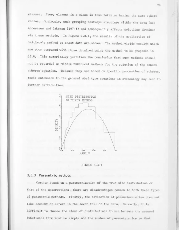
via these methods. In Figure 3.3.l , the results of the application of Saltikov's method to exact data are.shown. The method yields results which

are poor compared with those obtained using the method to be proposed in

§3.6. This numerically justifies the conclusion that such methods should

not be regarded as viable numerical methods for the solution of the random

spheres equation. Because they are based on specific properties of spheres,

their extension to the general Abel type equations in stereology may lead to

further difficulties.

g

.; _{SIZE DISTRIBUTIO} SALTIKOV METHOD

RADIUS

FIGURE 3.3.1

3.3.3 Parametric methods

Whether based on a parametrization of the true size distribution or

that of the observations, there are disadvantages common to both these types

of parametric methods. Firstly, the estimation of parameters often does not

take account of errors in the lower tail of the data. Secondly, it is

difficult to choose the class of distributions to use because the assumed

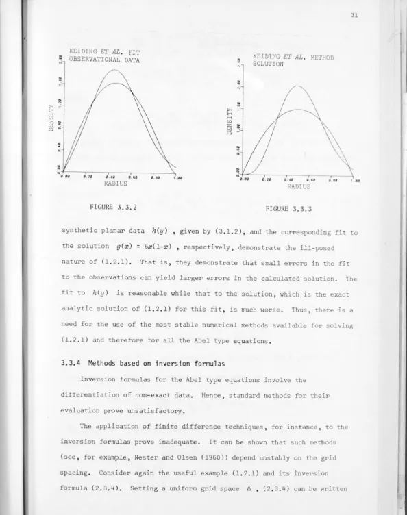
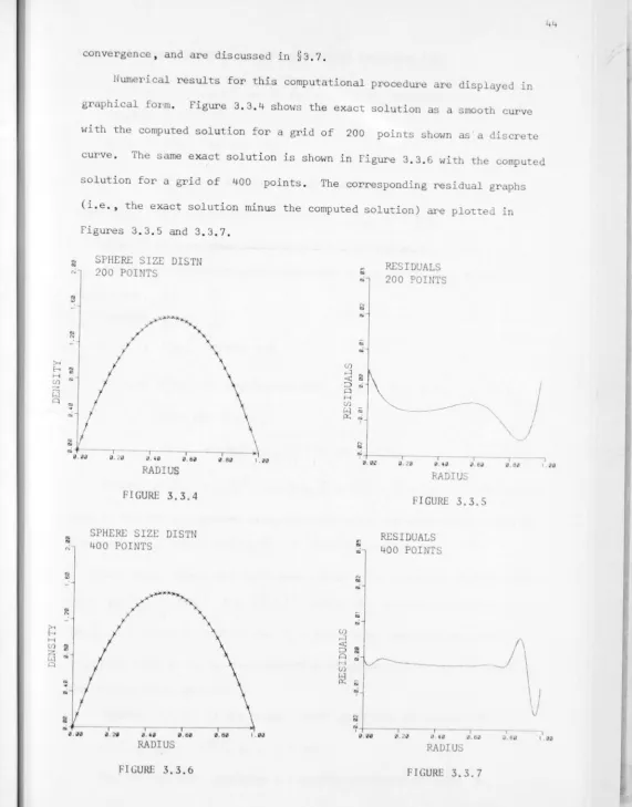
[image:36.623.32.613.19.763.2]

30

parameter estimation is numerically efficient.

Choosing a low number of parameters, however, produces a model which is

not widely applicable. For example, the logarithmiconormal probability

density considered by DeHoff (1965) is shown to be only a somewhat

reasonable global model when g(x) is a unimodal function with a skew

toward the domain of smaller particles (see DeHoff (1965)). Furthermore, the underlying parameter estimation method does not allow for truncated data, though it could be modified to do so.

A reasonable fit to the data could be obtained, if a larger number of parameters were used, but then the computational procedure would be, at best arduous, and at worst impossible, and certainly no more accurate than the

comparatively simple computational procedure proposed in this paper. In

solving (1.2,1) and (1.2.2), Keiding et al. (1972) use a parametrization of

the profile radius distribution based on assuming the sphere size

distribution is a Chi distribution with a degrees of freedom and scale

parameter b , viz.

[r

(f)

2 (a/2 )-lba/2]-\a-le -y

2

/2b •

They appear to have come the closest to optimizing the trade-off between efficiency and goodness of fit. The general computational complexity of

their maximum likelihood estimation, though, is still exceptionally higher

than that of the procedure to be proposed and the fit for given data is not

as close. They also take some account of truncated data assuming that unrecorded small profiles are derived from spheres the resultant contours of

which are small due to the angle at which they are sectioned.

In short then, most parametric models construct approximations which do

not fit nor represent the structure in the data accurately. The comments on the disadvantages of the pseudo-analytic models discussed in §3.3.4 also

apply here.

>-< r' H C/) :z; w Q

KEIDING E1' AL. FIT

~ OBSERVATIONAL DATA

i:!

-..

.,

..

~

..

"' "' RADIUS >, r' H C/) :z; w A

0.60 1.00

..

KEIDING E1' AL. _METHOD

"' SOLUTION

"'

..

..

"'

..

_~

-\

..

"' "' "'

..

"'

..

..

_{0.00 0.29 0. ,0}

[image:38.623.23.617.12.764.2]

0. 60 0.60 RADIUS

FIGURE 3,3,2 FIGURE 3,3.3

31

I. 00

synthetic planar data

h(y)

,

given by (3.1.2), and the corresponding fit to

the solution g(x) = 6x(l-x) , respectively, demonstrate the ill-posed

nature of (l.2.1). That is, they demonstrate that small errors in the fit

to the observations can yield larger errors in the calculated solution. The

fit to

h(y)

is reasonable while that to the solution, which is the exact

analytic solution of (l.2.1) for this fit, is much worse. Thus, there is a

need for the use of the most stable numerical methods available for solving

(l.2.1) and therefore for all the Abel type equations.

3.3.4 Methods based on inversion formulas

Inversion formulas for the Abel type equations involve the

differentiation of non-exact data. Hence, standard methods for their

evaluation prove unsatisfactory.

The application of finite difference techniques, for instance, to the

inversion formulas prove inadequate. It can be shown that such methods

(see, for example, Nester and Olsen (1960)) depend unstably on the grid

spacing. Consider again the useful example (l.2.1) and its inversion

g(x

.)

= g(i t,)

1,

where

= -2rrrib

Nr,l

I(j+l)t. [yh' (y )-h(y)] dy

TI • • • "

2 (

2

.

2" 2)

¾

J=1, Ju

y y

-1, u

(i =

o

,

1, ... , N)

.,.. N-1 f(j+l)t.

~ -2rmu

L ~

.

dy

TI J=1, • • J J.Ll " y

2(

y

2

-1,

.2,..2)f

Ll

(h. -h .)

~- = t,j J+l J

J t,

h. l+h.

J+

2 J = (j-¾)hJ+l . - (j+¾)h. J

represents a finite difference approximation to the term

[yh'(y)-h(y)J

32

If the approximation to

g

(x.)

is now integrated, the following quadrature 1,

rule is obtained:

where

and

with

-'2!11 N

g . = -ry;-

'°'

Q •. h . (

i

= 0, 1, ... , N)

i, Tii.u .L . i.J J

J =i.

Q .• = -(i+¾)P .. ,

1, 1, 1, 1,

Q. ·

=

(j-f)P. · l - (j+¾)P .. (j

=

i+l, ... , N-1)

1,J 1, ,J - 1,J

Q. N

1, '

= (N-})Pi N-1

'

[ .2 .2]J -1, ¾

j

If the values of

{hk}

are perturbed by the amount

{ohk} ,

then the

perturbations

{ogk}

in the solution are given by

'2m N

ogk = ~

z::

Q,,,;oh. <k =

o,

1, ... , N) .

j=k "<) J

The effect of a single perturbation

ohk

is

Og.

= 1,

0

i = O , l , ••• , k ,

i = k+l, .•. , N •

Thus, for a single perturbation

3 (2k+l)2

(k+1) ohk •

The amplification factor then is 0(6-1) . Clearly, if 6 is taken too

small, perturbations in

h(y)

can be amplified excessively. Yet if it is

not taken small enough, the truncation error associated with (3.3.7) will

be large, and hence _{will not be a good approximation to}

_{{g(x )}}

k ,

even for analytic data.

Because of this unstable dependence on 6 , these schemes are also

excluded from further consideration.

33

Other methods for Abel equations, based on inversion formulas, include

the

paeudo

-

anaZytic methods

of Minerbo and Levy (1969) (the M-L method),

Einarsson (1971), and Piessens and Verbaeten (1973). These methods are

based on the assumption that the solution can be represented by a finite

number of basis functions. The M-L method approximates the data in a least squares sense employing a polynomial fit for which the inversion is done

analytically. Via numerical experimentation, Minerbo and Levy (1969)

established that, for noisy data, their method was either better or compared

favourably with other suggested procedures. Recently, Einarrson (1971)

approximated the unknown function, g in our case, by a spline representation

with unknown parameters. In this method an overdetermined system of equations is set up. Some result from the condition that the continuity of the spline

approximation be satisfied exactly, while the remainder correspond to the

condition that the fit to the solution be determined by least squares.

Piessens and Verbaeten (1973) approximated the data using Chebyshev polynomials for which the inversion can be done analytically in terms of

generalized hypergeometric functions.

The least squares component in each of these three methods will be

effective in controlling noise in the data, if the smooth function used is

34

general, there is no guarantee that this condition is satisfied, since the methods are based on representations with a special sense or bias. Moreover,

use of an inappropriate representation for the structure in the data, even

though the fit is quite satisfactory, can yield a very poor approximation to

the solution. This is a ramification of the improperly posed nature of the Abel equation formulation; viz., certain types of small perturbations in the data can yield large perturbations in the solution (see Anderssen (1973) for a specific example, as well as the discussion of Figures 3.3.2 and 3.3.3 in §3.3.3 above), For these reasons, the use of pseudo-analytic methods (just like parametric methods) should only be made when independent arguments increasing their viability in a given context exist.

Anderssen (1973) proposes methods for Abel's equation based on the evaluation of the inversion formulas using product integration to evaluate

the integrals and spectral differentiation to determine the numerical derivatives (see Anderssen and Bloomfield (1974a, 1974b) for a complete discussion of spectral differentiation: a survey is given in §3.4). It is shown (see Anderssen (1973) and (1975)) that such methods consistently yield better results than the pseudo-analytic methods when applied to synthetic data.

The success of such schemes is largely due to the stable nature of spectral differentiation. It takes the structure within the data, {vk}

'

say, into account by filtering the noise

{Ek}

from the signal u(x) .

Thus, the procedure finds the derivative of u(x) with respect to the grid {xk} when { vk} is given by

vk=u(xk)+£k (k =0, 1 , 2 , ••• , N) . (3.3.8)

As mentioned in the Introduction §1.3, the only limitations on its use are conditions concerning the nature of the data. They are: