Theses Thesis/Dissertation Collections
2013
Implementation, integration, and optimization of a
fuzzy foreground segmentation system
Ryan M. Bowen
Follow this and additional works at:http://scholarworks.rit.edu/theses
This Thesis is brought to you for free and open access by the Thesis/Dissertation Collections at RIT Scholar Works. It has been accepted for inclusion in Theses by an authorized administrator of RIT Scholar Works. For more information, please [email protected].
Recommended Citation
Optimization of a Fuzzy Foreground
Segmentation System
by
Ryan M. Bowen
A Thesis Submitted in Partial Fulfillment of the Requirements for the Degree of Master of Science
in Computer Engineering
Supervised by
Associate Professor Dr. Ferat Sahin Department of Electrical Engineering Kate Gleason College of Engineering
Rochester Institute of Technology Rochester, New York
February 2013 Approved by:
Dr. Ferat Sahin, Associate Professor
Thesis Advisor, Department of Electrical Engineering
Dr. Juan Cockburn, Associate Professor
Committee Member, Department of Computer Engineering
Dr. Jay Yang, Associate Professor
Rochester Institute of Technology Kate Gleason College of Engineering
Title:
Implementation, Integration, and Optimization of a Fuzzy Foreground Segmentation System
I, Ryan M. Bowen, hereby grant permission to the Wallace Memorial Library to reproduce my thesis in whole or part.
Ryan M. Bowen
Dedication
I dedicate this work to my loving family and closest of friends that have truly inspired, supported, and at times carried me through my ever
Acknowledgments
Through the years there are many who I would like to express thanks. Above all, I am grateful for the guidance and generosity that has, and continues, to be provided by my advisor Dr. Ferat Sahin. His words of wisdom have found themselves contributing to the basis of my successes. This basis has found itself spanning some of the most important subsets of
my life; family, academia, integrity, and devotion.
I would like to thank Alexandra for providing the motivational support needed to complete this work, thank-you very much.
I would also like to convey special thanks to all my fellow research assistants at the Multi-Agent Bio-Robotics Laboratory. Each of you have
contributed your own unique roles in the completion of this work. Eyup, our initial project together was the true beginning of this whole
thing, thanks for the kick-start.
Vu, you have always been the man to count on and you have helped more than you even know, thanks.
Ticiano, our overlapping interests have provided a great friendly competition that has brought our algorithms to the next level, thanks. For Vince, a very special thanks is due for his uncanny ability to contribute
a fresh perspective, maintain perpetual candor, render an astonishing prowess to confound the obvious, and capacity to accommodate an
Abstract
Implementation, Integration, and Optimization of a Fuzzy Foreground Segmentation System
Ryan M. Bowen
Supervising Professor: Dr. Ferat Sahin
Contents
Dedication . . . iii
Acknowledgments . . . iv
Abstract . . . v
Glossary . . . xvi
1 Introduction . . . 1
1.1 Foreground Segmentation . . . 3
1.1.1 Fuzzy Image Processing . . . 5
1.2 Fuzzy Systems . . . 7
1.2.1 Fuzzifiers . . . 7
1.2.2 Rule-Based Fuzzy Models . . . 9
1.2.3 Mamdani Inference . . . 10
1.2.4 Defuzzification . . . 11
1.2.5 Multivariate Systems . . . 12
1.3 Real-Coded Genetic Algorithms . . . 13
1.3.1 Selection . . . 16
1.3.2 Crossover . . . 22
1.3.3 Mutation . . . 26
1.3.4 Replacement . . . 31
1.3.5 Convergence and Reinitialization . . . 32
1.4 System of Systems . . . 33
2 Proposed Method . . . 37
2.1 Pixel Representation . . . 38
2.2 Image Statistics . . . 39
2.3 Fuzzy Foreground Segmentation . . . 41
2.3.1 Fuzzification . . . 43
2.3.2 FIS Rule Base . . . 43
2.3.3 Defuzzification . . . 46
2.4 Filtering . . . 46
2.5 Segmentation . . . 48
2.6 System of Systems Architecture . . . 48
2.6.1 System of Systems Integration . . . 51
2.7 System Evaluation . . . 58
2.8 System Optimization . . . 59
2.8.1 Fitness Function . . . 59
2.8.2 Genetic Algorithm Selection . . . 61
3 Results . . . 66
3.1 Experimental Results of RCGA . . . 66
3.2 Optimization Results of FFSS . . . 76
3.3 Implementation of SoS . . . 83
3.3.1 Communication . . . 85
3.3.2 Software . . . 91
3.4 Application of FFSS . . . 95
4 Conclusions . . . 98
A Benchmark Functions . . . 108
A.1 Generalized Rosenbrock’s Function . . . 108
A.2 Generalized Rastrigin . . . 109
A.3 Generalized Griewangk . . . 109
A.4 Generalized Schwefel Problem 2.26 . . . 110
A.5 Ackley’s Function . . . 110
B RCGA Convergence Plots . . . 112
B.1 Rosenbrock . . . 112
B.2 Rastrigin . . . 114
B.3 Griewangk . . . 116
B.4 Schwefel . . . 118
B.5 Ackley . . . 120
List of Tables
1.1 Hypothetical fitness values and their corresponding
selec-tion probabilities and roulette wheel slot allocaselec-tion. . . 18 1.2 Comparison of proportionate, linear rank, and non-linear
rank selection probability distributions for a small example population. M is the size of the population andq is the se-lection pressure parameter used in the rank-based sese-lection
algorithms. . . 21 2.1 Assignment of membership functions to input per each rule
defined for the FIS. βi is the output of the rule and bi is the
value of the singleton fuzzy output assigned to it. . . 46 2.2 Problems and suggested actions for background maintenance
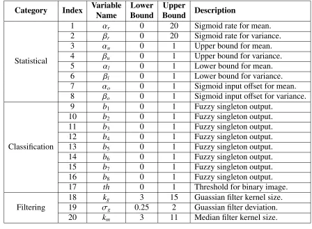
issues represented in the image sequences. . . 58 2.3 FFSS parameter list with domain ranges and parameter
de-scriptions. Their uses are described in their corresponding categorical sections of this work: statistical (Section 2.4 ),
classification (Section 2.3), and filtering (Section 2.4). . . 60 2.4 Different RCGA operators explored with their associated
parameters and corresponding bounds, where M is the pop-ulation size of the RCGA. Replacement operator not show
because greedy replacement was only considered. . . 62 3.1 Workstation used for execution of the RCGA during
3.2 Experiment settings for data collection of performance of
combinations of RCGA genetic operators. . . 68 3.3 RCGA settings used with experimentation of different
ge-netic operators. . . 68 3.4 Empirically found best combination of genetic operators and
parameters with respect to data collected for test functions. . 69 3.5 Manually selected operators and parameters for implemented
RCGA. . . 70 3.6 Average and standard deviation of the best fitness values
found by E-RCGA, M-RCGA, and algorithms as provided
by Yuen and Chow [55] : f1, f2 . . . 71
3.7 Average and standard deviation of the best fitness values found by E-RCGA, M-RCGA, and algorithms as provided
by Yuen and Chow [55] : f3, f4 . . . 71
3.8 Average and standard deviation of the best fitness values found by E-RCGA, M-RCGA, and algorithms as provided
by Yuen and Chow [55] : f5 . . . 72
3.9 Average and standard deviation of the best fitness values
found by E-RCGA, M-RCGA : f6 . . . 72
3.10 Derived fitness measure relative to average fitness values and standard deviations of test functions. Best performing
algorithms minimize (in bold) the derived fitness function. . 73 3.11 FFSS parameters optimized by the E-RCGA algorithm. The
full-set parameter represent the parameters used on all the image sequences, and the sub-set those for the sub-set
3.12 Number of false positive and false negative pixel classifica-tions for the FFSS algorithm and other algorithms presented
List of Figures
1.1 Components of a fuzzy rule-based system. . . 8 1.2 Fuzzy inference system membership implemented using a
Gaussian function. . . 9 1.3 Simple roulette wheel with 32 possible slots and each
hav-ing equal probability of selection. . . 18 1.4 Weighted roulette wheel based on selection probability as
obtained from Table 1.1. . . 19 1.5 Example of selection via roulette wheel scheme, where both
PDF and CDF are based on selection probabilities deter-mined by fitnesses of the individuals and X is a continuous
uniformly distributed random number. . . 19 1.6 Visual depiction of binary tournament selection with
diver-sity modification. Individuals are selected from previous ex-ample from Table 1.1 and X is a continuous, and uniformly distributed random variable. (a) Represents a tournament with selection of the better individual and (b) is a different
tournament with selection of the worse individual. . . 22 1.7 Example of uniform crossover for real-coded genetic
algo-rithms, whereαis the crossover rate andrare random
1.8 Uniform blended crossover with (a) static blending rate and (b) uniform random blending rate, where αis the crossover rate,r are random numbers used to evaluate crossover
crite-ria, andβare blending rate parameters. . . 25 1.9 Random mutation for real-coded genetic algorithms for a
sample set of offspring with mutation based on a static
mu-tation rate, γ = 0.05. . . 27 1.10 Creep mutation for real-coded genetic algorithms for (a) a
sample set of offspring with (b) mutation based on a static mutation rate, γ = 0.05, and (c) mutated values chosen based on normally distributed random numbers with a (d)
variation of σ2 =0.25. . . 28 1.11 Adaptive mutation sigmoid functions with different λ andτ
values as defined by Equation 1.29, where γmax = 0.1 and
γmin = 0.001. . . 31
2.1 Adaptive weighting parameter sigmoid functions with dif-ferent characteristics as defined by Equations 2.7, and 2.8, where r, u, l, o, respectively represents parameters for α/β,
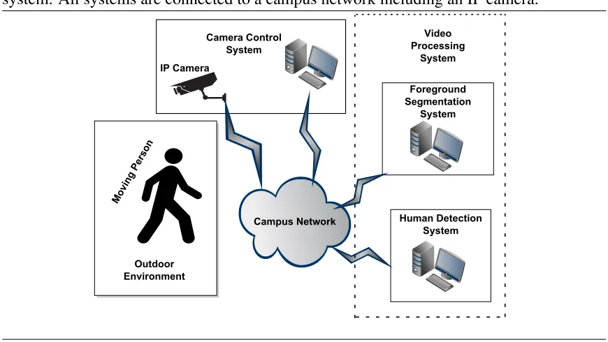
and z[n] is a pixel’s belongingness to foreground. . . 42 2.2 Block diagram of the overall foreground segmentation system. 43 2.3 Diagram of all the individual systems that compose the
over-all human detection system. All systems are connected to a
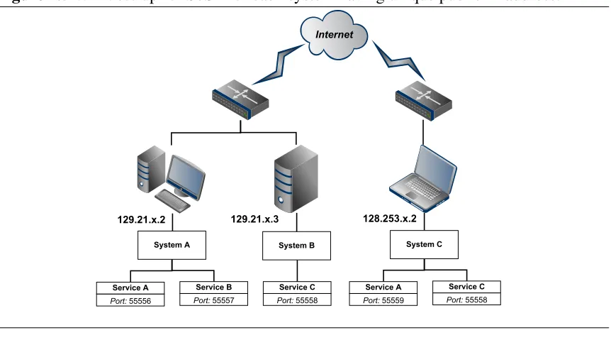
campus network including an IP camera. . . 49 2.4 LAN set-up for SoS with each system having unique private
IP address. . . 55 2.5 WAN set-up for SoS with each system having unique public
2.6 LAN set-up for SoS where some systems share a common
private IP address. . . 56
3.1 Comparison of optimization algorithms base on derived fit-ness measure relative to average fitfit-ness values and standard deviations of test functions. Best performing algorithms minimize the derived fitness function. . . 74
3.2 Execution time comparison of E-RCGA and M-RCGA for 100 trials with 40,100 fitness evaluations at 10, 20, 30, 40, and 50 dimensions. . . 75
3.3 Convergence plots for test function (a) Rosenbrock, (b) Ras-trigin, (c) Griewangk, (d) Schwefel, (e) Ackley, and (f) Michalewicz. Average fitness values are reported per generation per 100 trials a on log-scale. . . 77
3.4 Sigmoid mapping function α for weighting used for calcu-lating the accumulated mean for a pixel. . . 79
3.5 Sigmoid mapping function β for weighting used for calcu-lating the accumulated variance for pixel. . . 79
3.6 Binary foreground images for FFSS and other algorithms as presented by Toyama et al. [48] . . . 81
3.7 False positive and false negative comparison for the full set of image sequences. . . 82
3.8 False positive and false negative comparison for the sub-set of image sequences. . . 82
3.9 Hierarchy of the implemented SoS. . . 84
3.10 WAN Setup. . . 85
3.11 Sequence diagram for communication initialization . . . 89
3.13 Service hierarchy used to implement the different service
types within the human detection SoS. . . 93 3.14 Frame Grabber hierarchy used to provide modularity for
various image input sources. . . 94 3.15 General relationships of the different entities used to
repre-sent the SoS in software. . . 94 3.16 FFSS-Full results of (a) current image, (b) fuzzy control
im-age, (c) foreground segmented imim-age, (d) human detection
image. . . 96 3.17 FFSS-Sub results of (a) current image, (b) fuzzy control
im-age, (c) foreground segmented imim-age, (d) human detection
Chapter 1
Introduction
The motivation for this work stems from a common problem of developing an automated system to detect a human within a series of sequential im-age sequences. Human detection systems are of high interest to numerous applications especially video surveillance. Utilizing an automated human detection system can eliminate the requirement for human-based surveil-lance practices and potentially increase productivity. Upon investigation of implementing such an automated system, a holistic view suggests that mul-tiple complex systems are required to independently operate and interoper-ate with each other. From a top level hierarchical view, a human detection system can be decoupled into a system for obtaining images, a system for implementing image processing, and a system for executing some behavior based on current system status. Each of these systems could then contain sub-systems to reduce their overall complexity and provide some modu-larity. Due to the complexity and sheer size a complete human detection system, improving upon all required sub-systems is not practical. There-fore, the focus of this work is placed on improving the image processing system. Additionally, the image processing system is investigated from a general standpoint such that it may be applied to applications other than human detection.
to accurately classify pixels as foreground can be vital to the performance of many object detection algorithms. Therefore, this work is more specifically an investigation into the design, implementation, and application of a novel foreground segmentation system.
The proposed solution to the foreground segmentation problem is the re-alization of a Fuzzy Foreground Segmentation System (FFSS). The primary goal of the FFSS is to reduce false classification of foreground pixels. To achieve better classification, Mamdani-type Fuzzy Inference Systems (FIS) are used at the pixel-level. The membership functions for each FIS are Gaussian distributions with inputs of pixel component values. Additionally, the membership functions are dynamic, changing shape according to accu-mulating estimations of a pixel’s mean and variation. Through the use of a FIS, the definition of the control algorithm is simplified via the use of logical words such ashighandlow. Moreover, the output of the FIS is able to better control accumulating pixel statistics which in turn are used for classification of pixels as foreground.
Evaluation of the FFSS is primarily focused on the accuracy of clas-sifying foreground pixels. Different standard image sequences represent-ing different canonical problems are used to test the accuracy of the FFSS. Ground truths for these image sequences have been provided for specific image frames within the sequences. The FFSS will be executed on each image sequence and compared to their respective ground truths. The FFSS performance with respect to an image sequence is quantified by summing the number of false positives (pixel detected as foreground when it should have been background) and false negatives (pixel detected as background when it should have been foreground) for a specific image frame in time.
RCGA schema and their performance on several multi-dimensional func-tions. The chosen multi-dimensional functions are specifically designed for benchmarking optimization algorithms and represent various functions landscapes. The best schema is chosen as the one that minimizes conver-gence time while maximizing accuracy and repeatability. Furthermore, the RCGA’s performance on the benchmark functions is qualified by compari-son to other existing optimization algorithms.
The importance of foreground segmentation is demonstrated by imple-menting a real-world application; detection of a moving human within se-quential single perspective images. This application of a Human Detection System (HDS), is composed of multiple heterogeneous systems such as an Internet Protocol (IP) camera, a computer for communicating to the camera, and computer(s) for implementing the different individual image processing sub-systems. Due to the multiple systems involved, a System of Systems (SoS) architecture is used to decompose the complex system into multiple simpler systems coupled together via self-describing XML data exchange over Ethernet using TCP/IP.
1.1
Foreground Segmentation
Foreground segmentation plays an important role in many video process-ing algorithms. It is typically a preliminary step for more complex image processing methods such as object detection. Reviewing current research pertaining to foreground segmentation (also referred to as background sub-traction or foreground detection), the process is found to be typically com-posed of 1) obtaining a model representing the background scene and 2) classifying foreground objects as those deviant from the background model. Therefore, in order for the proposed FFSS to be successful it must be ca-pable of producing an accurate estimate of a background model as well as accurately classify current pixels.
from a background model, but instead affect the process of maintaining the background model itself. The importance of obtaining an accurate, robust, and efficient background modeling algorithm has lead to numerous meth-ods such as frame differencing, mean and threshold, mixture of Gaussians [19], Bayesian decision [34], eigen background [35], linear predictor, and wallflower [48]. Toyama et al. have established a database of seven image sequences to model specific canonical problems associated with background modeling. These image sequences were then used to test the performance of the previously listed background maintenance algorithms. The performance results of the various algorithms, as recorded by Tomaya et al., will be used to provide a metric for the performance of the proposed FFSS.
The background modeling process should also consider the color space and how color components should be used represent pixel values. RGB is the most common color space used by video capturing devices. However, when considering image processing techniques, the RGB color space has it disadvantages with correlation between its three color component (R,G,B). The RGB color space is very susceptible to changes in illumination, as il-lumination affects all three components of the RGB color space. There-fore, other color spaces that are capable of isolating illumination from other color components are suggested. Horprasert et al. [22] has proposed a back-ground subtraction method using the RGB color space, the Pfinder [53] sys-tem from MIT uses YUV and Zhao et al. [59] have used the HSV color space. From these background implementation, the HSV color space shows promising results with increased stability due to its ability to separate bright-ness from chromaticity [59]. Initial work using the HSV color space has been demonstrated [7] and appear suitable for the proposed FFSS. However, the non-linearity and periodicity of the Hue channel could provide instabil-ity in the background model, thus investigation of the YCrCb is shown in this work.
or adaptive filters have been used to continually build the background model [53, 29]. The proposed FFSS will make use of accumulating statistics as to not only reduce memory requirements, but to also improve robustness through the adaptability of running statistical models. The weighting factor used in accumulating statistics will be allowed to change with respect to the degree of foreground classification. This adaptive feature is intended to allow the background model to respond to environmental changes.
Classification of foreground pixels is typically achieved by analyzing a pixel’s variance from an estimated background model. A pixel’s belonging to foreground or background is then determined by a probability distribu-tion(s) where Gaussian distributions are typical. As similar to the mixture of Gaussians method [19], the FFSS will use multiple weighted Gaussian distributions to determine a pixel’s probability of being classified as fore-ground. However, the FFSS Gaussian distributions will be defined by a Fuzzy Inference System (FIS) and output weighting will be achieved using a set of fuzzy rules. Chua et al. have shown success with their fuzzy rule-based system for background subtraction [12]. Similar to this work, Chua et al. classify foreground pixels as those deviant from the background and thus focus on background maintenance. Chua et al. differ from this work by using texture and gradient information of pixel in addition to color for the input of their fuzzy rule-based system. Chua et al. use a visual and nu-merical F-Measure to compare results to other algorithms on 9 different test sequences (3 of these from the wallflower dataset). Chua et. al demonstrate excellent based on their numerical measure, however image sequences were chosen based on an assumption of dynamic textures for scenery.
1.1.1 Fuzzy Image Processing
Therefore, fuzzy sets have been applied to image processing for better rep-resentation of uncertainty in crisp or quantized numbers [27, 51, 29] and to improve the accuracy of object/pixel classification [41, 2]. The proposed FFSS will make use of fuzzy sets to represent each pixel’s belongingness to the foreground.
Jawahar and Ray have used first and second order fuzzy statistics to better represent the spatial gray-level distribution of a digital images [27]. Jawahar and Ray represent fuzzy sets with triangular membership functions, where a each pixel’s gray-level is quantified according its belonging to the triangu-lar membership (fuzzy number). The fuzzy numbers are then used to create a fuzzy histogram that represents the distribution of gray-levels of an im-age. In comparison to hard histograms, the fuzzy histograms were able to provide a better representation of an image’s gray-level frequency distribu-tion due to their ability to incorporate gray-level imprecision. Vlachos and Sergiadis [51] further the use of Jawahar and Ray’s notion of a fuzzy his-togram except they use higher-order intuitionistic fuzzy sets (IFS) to model the indeterminacy in image pixels. The FFSS proposed will expand upon Jawahar and Ray’s work by investigating the use of guassian memberships as opposed to triangular memberships.
Chacon et al. define and apply a fuzzy image processing scheme to edge detection, object geometry measurement under varying illumination con-ditions. Chacon et al. outline the process of fuzzy image processing as defining a fuzzification functions to convert from the spacial domain to the fuzzy domain, defining fuzzy operators to perform mathematical expres-sion within the fuzzy domain, and defuzzification functions for visualiza-tion and/or extracting useful information [11]. This process as outlined by Chacon et al. will be adopted and used to design and implement the FFSS.
robustness and ability to used in outdoor application or any location with changing illumination.
Sigari et al. provide methods for using fuzzy accumulating statistics as a precursor for background subtraction [29]. The fuzzy running average by Sigari et al. was applied to vehicle detection on a highway, and it demon-strated improvement over the classic running average method especially under extensive illumination changes and high vehicle density. However, Sigrai et al.’s segmentation of the foreground is limited to simple threhold-ing with a threshold value found usthrehold-ing trial and error. Shakeri et al. im-proved upon the background subtraction by using fuzzy inference in combi-nation with cellular automata [41]. As mentioned previously, the FFSS will use accumulating statistics, however improvement on classic accumulating statistics will be achieved through the use of fuzzy mapping functions [29].
1.2
Fuzzy Systems
Fuzzy systems make use of input variables that are represented as fuzzy sets as oppose to crisp values. These fuzzy sets are used to attempt to quantify some uncertainty, imprecision, ambiguity, or vagueness that may be associ-ated with a variable. Commonly, these fuzzy systems are defined by using
if-then rules also referred to as rule-based fuzzy systems [3]. The output of fuzzy systems have been used for modeling, data analysis, prediction and control. Regardless of the final application the basic system output stems from the fuzzy model itself. A rule-based fuzzy system can be described through the use of four sub-systems including a Fuzzier, Fuzzy Rule Base,
Fuzzy Inference System, and aDefuzzifier as shown in Figure 1.1.
1.2.1 Fuzzifiers
Figure 1.1Components of a fuzzy rule-based system.
Fuzzifier
Fuzzy Rule Base
Fuzzy Inference
System Defuzzifier
Fuzzy Sets in U Fuzzy Sets in V
x in U y in V
INPUT OUTPUT
inference system. There are three popular fuzzifiers that are used, single-ton, Gaussian, and triangular. For the focus of this work the singleton and Gaussian fuzzifiers are discussed.
˜
x ∈U ⊂ Rn → A0 ∈ U (1.1)
The singleton fuzzy set is a fuzzy set with support at a single point, x∗, inU
with a membership function of one:
µA0(x) =
1 x = x∗
0 ∀ x ∈U | x , x∗ (1.2)
The Gaussian membership function as seen in Figure 1.2 is defined as:
µ= exp
−(x−c)2 2σ2
Figure 1.2Fuzzy inference system membership implemented using a Gaussian function.
0 0.25 0.5 0.75 1
-3σ -2σ -σ c σ 2σ 3σ
F
uzzy
Output,
µ
(0
,
1)
Input,x (0,1)
Fuzzy Inference System Gaussian Membership Function
µ(x)
1.2.2 Rule-Based Fuzzy Models
For rule-based fuzzy systems, variables and their corresponding relation-ships are modeled through the means of fuzzy if-thenrules [3]. The general form of these if-thenrules are:
Ifantecedent proposition then consequent proposition
Based on the form of the consequent there are two main rule-based models:
• Linguistic fuzzy model: both antecedent and consequent are fuzzy propo-sition [56, 30].
• Takagi-Sugeno (TS) fuzzy model: the antecedent is a fuzzy proposition and the consequent is a crisp function [44].
For the focus of this work the linguistic fuzzy model, as introduced by Mamdani [30], will be used to form qualitative models from if-then rules. The general form of the linguistic fuzzy model if-then rules as described by Babuska is:
Where ˜x is the input (antecedent) linguistic variable, and Ai are the
an-tecedent linguistic values of ˜x. The output (consequent) linguistic variable is represented as ˜ywithBi corresponding to the consequent linguistic values
of ˜y. The values ˜xand ˜yare fuzzy sets defined in their respective domains :
x ∈ X ⊂ Rp and y ∈ Y ⊂ Rq. The membership functions of the antecedent and consequence fuzzy sets are: µ(x) : X → [0,1], µ(y) : Y → [0,1]. The linguistic terms, Ai, are fuzzy sets that defines the fuzzy region in the
antecedent space for respective consequent propositions. Ai and Bi are
typi-cally predefined sets with terms such asLarge,Small, etc. Using Aand Bto denote these predefined sets, respectively we have Ai ∈ Aand Bi ∈ B. In all,
the knowledge base of the fuzzy linguistic model is composed of the rule
base R = {Ri|i = 1,2, . . . ,K} and setsA and B.
There is a special case of fuzzy linguistic model that usessingletonfuzzy sets to represent the consequent fuzzy set. If Bi is a fuzzy singleton set with
support ˜ythen:
µB0i(y) =
1 y =y˜
0 ∀ y∈ Y | y, y˜ (1.5) With the use of singleton fuzzy sets as the output (consequent fuzzy sets), these singleton sets can be represented as real numbers bi, simplifying the
rules generalization:
Ri : If x˜ is Ai theny = bi, i = 1,2, . . .K (1.6)
1.2.3 Mamdani Inference
The rules as generally defined in Equation 1.4 can be expressed as a fuzzy relation : Ri : (X ×Y) → [0,1]. For the focus of this work, the fuzzy relation
minimum (∧) operator:
Ri =Ai× Bi
or
µRi(x,y) =µAi(x)∧µBi(y) (1.7)
The fuzzy relation R that represents the entire model can be formed by the union of the K individual rule relations Ri:
R =
K
[
i=1 Ri
or
µR(x,y) = max
1<i<K
µ
Ai(x)∧µBi(y)
(1.8)
Using Mamdani’s inference method, the output of a rule-based fuzzy model is computed by using max-min relation composition. Given that an input fuzzy value ˜x = A0, then its output value B0 is given by:
µB0(y) = max
X
h
µA0
i (x)∧µR(x,y) i
(1.9) From Equation 1.8 µR(x,y) can be substituted. Additionally, since max and
min operations are across different domains, their order can be changed. The final output membership are defined as:
µB0(y) = max
1<i<K
β
i ∧µBi(y) ,
y ∈Y (1.10)
where βi, as defined by Babuska, is thedegree of fulfilment of the ith rule’s
antecedent, denoted:
βi =max
X
h
µA0i (x)∧µAi(x) i
(1.11)
1.2.4 Defuzzification
Mamdani inference scheme is the center of gravity (COG) method. This method will compute a crisp valuey0 that represents the center of gravity of the area under the fuzzy set B0:
y0 =cog B0 =
F
P
j=1
µB0
yj
yj
F
P
j=1
µB0
yj
(1.12)
where F is the number of yj elements in Y. The COG equation provided
in Equation 1.12 is formulated for discrete Y domains. If a continuous Y
domain is used, then another form of the COG method should be used or the Y domain must be discretized.
If singleton fuzzy sets are used for the output of the system, then a sim-plified defuzzification method called thefuzzy meanmay be used. The fuzzy mean simplifies the fuzzy inference and the defuzzification methods into a single simple formula:
y0 =
K
P
i=1
βibi
K
P
i=1
βi
(1.13)
where Bi is the fuzzy fulfilment of the ith rule’s antecedent as expresses in
Equation 1.11.
1.2.5 Multivariate Systems
For the case of MIMO or MISO systems, it is easier to define the antecedent and consequent propositions as combinations of univariate fuzzy proposi-tions. To combine the propositions, common logic operators are used such as conjunction, disjunction and negation. Therefore, the rules for a MISO system can be generalized:
where, i = 1,2, . . . ,K. In this case the degree of fulfilment is given by:
βi = µAi1(x1)∧µAi2(x2)∧ · · · ∧µAip
xp
, 1 ≤i ≤ K (1.15)
1.3
Real-Coded Genetic Algorithms
There are many practical problems that exist that require systems with nu-merous inputs with complex interactions. Typically these problems present hard optimization problems and lack fast and optimal optimization algo-rithms. However, algorithms have been developed to achieve sub-optimal solutions to these hard optimization problems. Among these algorithms some of the more common are hill climbing, simulated annealing , ge-netic algorithms, particle swarm optimization, and scatter-search [32]. Each of the optimization algorithms have their own unique approach to sam-pling and representing a problem’s parameter space. Therefore, optimiza-tion methods will demonstrate variaoptimiza-tion in quality and execuoptimiza-tion time of their sub-optimal solutions. Hence, the selection of an optimization algo-rithm is highly dependant on the problem to be optimized. For this work Real-Coded Genetic Algorithms (RCGA) have been chosen as the optimiza-tion algorithm.
The RCGA was chosen as the optimization algorithm mainly due to its faster convergence in comparison to other optimization algorithms such as Particle Swarm Optimization (PSO) and scatter search. Additionally, in comparison to hill climbing, simulated annealing, and nelder-mead, genetic algorithms are less likely to prematurely converge in local minima. Further-more, the RCGA uses real-code values and better represents the application of this work; one that uses real-coded parameters. Lastly, the diverse set of operators available to the RCGA allow it to be re-configured based on the problem and desired algorithm performance.
sets of input parameters with each parameter representing an allele, the en-vironment is the system itself, and fitness is an evaluation function of the system input and output determined by optimization criteria. The genetic adaptive plan, is mathematically formalized by Holland with a framework introducing the concept ofschemaand providing a generalization ofgenetic operators [21]. These genetic operators are generalized through the use of genetic plans or reproductive plans based primarily on observed natural sys-tems. The set of genetic operators introduced by Holland includecross-over
andmutation, where cross-over is used to produce recombinations of alleles via exchange of segments of paired chromosomes and mutation is used to randomly replace or modify an allele based on some small probability dis-tribution. With these generalized genetic operators, reproductive plans can be developed to select chromosomes from the population, modify them, ap-ply operators to form new chromosomes (offspring), evaluate chromosome fitness and then repeat until some convergence criteria is satisfied.
Since Holland’s original formalized framework, extensive work has been done with respect to reproductive plans for genetic algorithms. Large fo-cus has been placed on the importance of selection in a reproductive plan. DeJong provided a standard method of selection such that the number of offspring attributed by an individual is proportional to its performance with respect to others in the population [13]. Baker proposes a ranking selection scheme where individuals contribute to a number of offspring based on rel-ative rank of performance in the population as opposed to their magnitude of performance [4]. A stochastic tournament selection schemes was sug-gested by Brindle where individuals are chosen for reproduction based on higher fitnesses of paired match-ups [10]. To better understand the impact of these common selection schemes, Goldberg and Deb provide a detailed analysis of these selection schemes with respect to time convergence using computer simulations of the individual selection schemes as applied to the k-armed bandit problem [18]. Sivaraj and Ravichandran, provide a holistic review of modern selection schemes where the majority of the schemes are slight modifications of the original proportionate selection, ranking selec-tion, or tournament selection schemes [42].
in 1975, new methods of data representation have been established along with new operators. Classically chromosomes of a genetic algorithm are represented as binary bit strings however Goldberg suggests the consider-ation of real-coded algorithms where chromosomes are represented using floating point or some other high-cardinality coding scheme [18]. Addi-tionally, Janikow and Michalewicz experimentally demonstrated faster ex-ecution time, reduction in variation, and increased precision when using a real-coded genetic algorithm as compared to one with binary-coding [26]. However, with real-coded genetic algorithms, special operators for cross-over and mutation are needed to deal with real parameters. Michalewicz defines simple real-coded implementations of crossover and mutation as analogous to the binary versions, where crossover and mutation operations are done at the parameter-level instead of the bit-level [32]. A thorough re-view and analysis of multiple real-coded crossover operators is provided by Ortiz-Boyer et al. [36].
Genetic algorithms are very versatile as for they can be implemented us-ing different encoding schemes, selection schemes, and with various genetic operators for recombination and mutation. However, the general outline of the execution of a genetic algorithm can be summarized as:
Procedure 1.1Genetic Algorithm
Input: Fitness Function
Input: Convergence Criteria
Output: Variable values that maximize fitness function
1: Random Initialization of Population
2: whileNOT Convergence Criteriado 3: Selection
4: Crossover
5: Mutation 6: Replacement
7: Possible Reinitialization
1.3.1 Selection
The selection operator for a genetic algorithm can be simply defined as the choosing of individuals to be involved in the process of reproduction with other individuals within the population as to produce new offspring. Those individuals chosen for reproduction form what is commonly referred to as a mating pool. Within a population of size, M, the members of the pop-ulation available for selection during generation, t, are noted as At; where
a single individual is represented as ai,t. Therefore, the goal of the
selec-tion process is simulate a process to naturally sample At, such that Lmating
pairs are formed from the selected mating pool. The diversity of the mating pool directly affects the convergence rate of a population throughout nu-merous generations. A highly diverse mating pool reduces the probability of the event that a generation of a population will converge to a single or limited number of individual(s). In turn, a diverse mating pool increases the likelihood of finding the globally best individual or global solution. More-over, a diverse mating pool will increase the number of generations required for a population reach convergence, leading to longer execution times. In contrast, a highly homogeneous mating pool can reduce the number of gen-erations required for a population to converge, but increases the risk of pre-mature convergence on an individual that may not be considered the global best or otherwise considered a local solution. There are a variety of selec-tion schemes that may be used to simulate the selecselec-tion process. Three of the most common schemes as discussed by Goldberg and Deb [18] are:
1. Proportionate Reproduction 2. Ranking Selection
3. Tournament Selection
Proportionate Reproduction
probability, psel, of an individual,ai,t, can be described as:
psel ai,t =
f ai,t M
P
i=1
f ai,t
(1.16)
where f is the objective function to be optimized at its global maxima [13]. However, it is common that an objective function is not optimized at its global maxima but instead at its global mimima. Therefore, it is necessary use the inverse of objective function, f−1, where
f−1 ai,t =
1
f ai,t
(1.17)
To reduce confusion, all explanations and definitions will pertain to fitness functions that are optimized at global maxima, but it is important to note that for some objective functions the inverse must be used.
Roulette Wheel Selection
In order to make use of the selection probability distribution it must be used in conjunction with a method of sampling the probability distribution. The sampling process can be executed using a variety of methods, however the mostly used is a variation of the roulette wheel selection scheme. The basic concept behind a roulette wheel is to spin a wheel with a predetermined number of slots, as seen in Figure 1.3, then to drop a ball into the spinning wheel and the slot the ball lands into is chosen as the winner. To use the roulette wheel as a sampling method, a weighted roulette wheel is used such that the size of the slots are proportional to selection probabilities. To help illustrate the creation of the weighed roulette wheel, Table 1.1 shows five hypothetical members of a population and their corresponding fitnesses and selection probabilities.
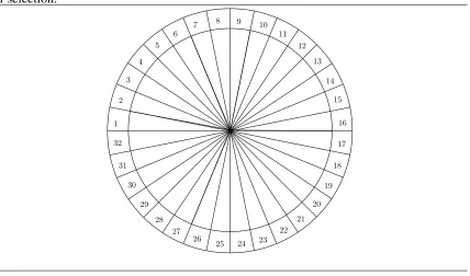
Figure 1.3Simple roulette wheel with 32 possible slots and each having equal probability of selection. 1 2 3 4 5 6
7 8 9 10
11 12 13 14 15 16 17 18 19 20 21 22 23 24 25 26 27 28 29 30 31 32
Table 1.1 Hypothetical fitness values and their corresponding selection probabilities and roulette wheel slot allocation.
a f(ai) psel(ai) No. Slots
a1 20 0.20 6
a2 35 0.35 11
a3 18 0.18 6
a4 11 0.11 4
a5 16 0.16 5
Totals: 100 1.00 32
Figure 1.4Weighted roulette wheel based on selection probability as obtained from Table 1.1. a4 a2 a1 a5 a3 35% 20% 18% 11% 16% 1 2 3 4 5 6 7
8 9 10 11 12 13 14 15 16 17 18 19 20 21 22 23 24 25 26 27 28 29 30 31 32
Figure 1.5 Example of selection via roulette wheel scheme, where both PDF and CDF are based on selection probabilities determined by fitnesses of the individuals and X is a continuous uniformly distributed random number.
0.35 0.20 0.18 0.16 0.11
0.35 0.55 0.73 0.89 1.00
a2 a1 a3 a5 a4
CDF X = 0.62
individual from At via the roulette wheel selection scheme is described in
Procedure 1.2, where psel ai,t is the selection probability of a single
indi-vidual in At.
Ranking Selection
The ranking selection scheme as introduced by Baker [4], is similar to that of the roulette wheel selection, differing only in the computation of the se-lection probabilities. Ranking sese-lection reduces the sese-lection pressure for
Procedure 1.2RouletteWheelSelection
Input: f(At) - Decendingly sorted array of fitnesses of all individuals.
Output: Index of the selected individual.
1: X ∼U(0,1) : P(X[x,x+d])= Rxx+ddy =dwhered >0
comment: Xrepresents continuous, uniformly distributed, random numbers.
2: sum←0
3: for allai,tdo
4: sum← sum+ psel ai,t
5: if x> sumthen
6: return i
7: end if
8: end for
Michalewicz specifies functions that utilize a single parameter q to de-fine linear and non-linear rank-based probabilities for individuals within a population [32]. The linear rank selection probability for an individual can be defined as:
prank =q 1−
rank−1
M −1
!
(1.18) and non-linear as:
prank =q(1−q)rank
−1 (1.19)
where M is the size of the population and rank [1,M] (rank = 1 is the best individual and rank = M is the worst individual). The single parame-ter, q, is used to adjust the selection pressure of the algorithm for both the linear and non-linear functions. Larger values of qimply stronger selection pressures which reduce the probability of less fit individuals to be selected for reproduction. For the linear function the typical range as suggested by Michalewicz is between M1 and M2 . However, for the non-linear function,
q (0,1), is not dependant on population size.
Table 1.2 Comparison of proportionate, linear rank, and non-linear rank selection proba-bility distributions for a small example population. Mis the size of the population andqis the selection pressure parameter used in the rank-based selection algorithms.
q= M1 q= M2 (q=0.1) (q= 0.6) Rank Fitness Proportionate Linear Linear Non-Linear Non-Linear
1 35 0.350 0.200 0.400 0.100 0.600
2 20 0.200 0.150 0.300 0.090 0.240
3 18 0.180 0.100 0.200 0.081 0.096
4 16 0.160 0.050 0.100 0.066 0.038
5 11 0.110 0.000 0.000 0.073 0.015
Tournament Selection
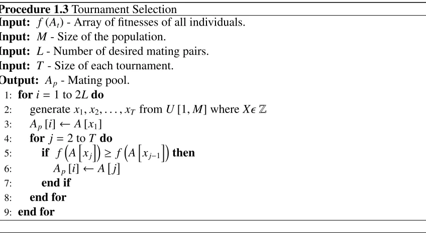
Tournament selection was initially investigated by Brindle [10] as unpub-lished work and also more recently studied by Goldberg and Deb [18]. Tour-nament selection is a simple process of choosing a number individuals ran-domly from a population, where the number of individuals chosen defines the tournament’s size. From the chosen individuals, the best fit individual is selected for further genetic processing, and thus concludes a tournament. This process is typically repeated till a desired number of best individuals are chosen such that a mating pool is filled. Procedure 1.3 provides a generic procedure to implementing the tournament selection process, as described above. Special consideration should be taken when selecting the size of the tournaments, since tournament size directly affects the diversity of the mat-ing pool. Smaller tournament sizes promote a diverse matmat-ing pool, whereas larger tournament sizes tend to create a more homogeneous mating pool with only better fit individuals.
Procedure 1.3Tournament Selection
Input: f(At) - Array of fitnesses of all individuals.
Input: M- Size of the population.
Input: L- Number of desired mating pairs.
Input: T - Size of each tournament.
Output: Ap - Mating pool.
1: fori=1 to 2Ldo
2: generate x1,x2, . . . ,xT fromU[1,M] whereX Z
3: Ap[i]← A[x1] 4: for j=2 toT do 5: if fAhxj
i
≥ f Ahxj−1
i
then 6: Ap[i]← Aj
7: end if
8: end for
[image:39.612.96.520.88.320.2]9: end for
Figure 1.6 Visual depiction of binary tournament selection with diversity modification. Individuals are selected from previous example from Table 1.1 andX is a continuous, and uniformly distributed random variable. (a) Represents a tournament with selection of the better individual and (b) is a different tournament with selection of the worse individual.
a
3a
1a
5a
4f(a3) = 18
f(a4) = 11
X= 0.65
a
3
(a)
f(a1) = 20
f(a5) = 16
X= 0.28
a
5
(b)
X≥0.5 X <0.5
of the population. This can be implemented by randomly selecting which individual of the binary tournament to place into the population (better or worse) as depicted in Figure 1.6 and outlined in Procedure 1.4.
1.3.2 Crossover
Procedure 1.4Binary Tournament Selection
Input: f(At) - Array of fitnesses of all individuals.
Input: M- Size of the population.
Input: L- Number of desired mating pairs.
Output: Ap - Mating pool.
1: fori=1 to 2Ldo
2: generate xfromU(0,1) whereXR
3: generate x1,x2fromU[1,M] whereX Z 4: if f (A[x1])≥ f(A[x2])then
5: if x≥ 0.5then 6: Ap[i]← A[x1]
7: else
8: Ap[i]← A[x2]
9: end if
10: else
11: if x≥ 0.5then 12: Ap[i]← A[x2]
13: else
14: Ap[i]← A[x1]
15: end if
16: end if 17: end for
operators for real-coded genetic algorithms are typically allowed to occur only between elements (parameters) as opposed to the bit-level as tradi-tional binary-coded genetic algorithms. By only operating between ele-ments, crossover using floating point numbers is quite analogous to binary implementations. The traditional crossover operator techniques are single-point,multi-point, anduniform crossover.
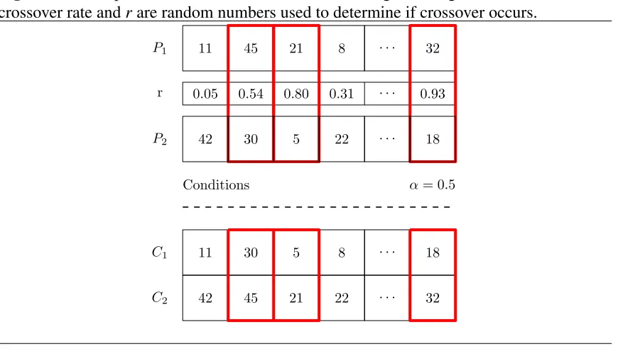
Figure 1.7Example of uniform crossover for real-coded genetic algorithms, whereαis the crossover rate andrare random numbers used to determine if crossover occurs.
11 45 21 8 · · · 32
P1
0.05 0.54 0.80 0.31 · · · 0.93
r
11
21
· · · C1
42 45 · · · 32
C2 22
8
30 5 18
α= 0.5 Conditions
42 30 5 22 · · · 18
P2
Uniform Crossover
In real-coded genetic algorithms, each gene represents an entire element or parameter. By operating at this elemental level, the typical crossover operators are semantically similar to their binary counter parts. For this sec-tion, P1, P2correspond to individual chromosomes paired for mating or
par-ents and C1, C2 represent the offspring produced after crossover. Uniform
crossover for real-coded genetic algorithms can be applied traditionally, as seen in Figure 1.7. In this case each gene or element is exchanged in whole between parents based on a static crossover rate (α).
Blended Crossover
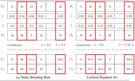
Figure 1.8 Uniform blended crossover with (a) static blending rate and (b) uniform ran-dom blending rate, whereαis the crossover rate, r are random numbers used to evaluate crossover criteria, andβare blending rate parameters.
11 45 21 8 · · · 32
P1
42 30 5 22 · · · 18
P2
0.05 0.54 0.80 0.31 · · · 0.93
r
11
14.6
· · · C1
42 39 · · · 20.1
C2 22
8
36 11.4 23.6
0.4 · · ·
β
α= 0.5
Conditions: β= 0.4
0.4 0.4 0.4 0.4
11 45 21 8 · · · 32
P1
42 30 5 22 · · · 18
P2
0.05 0.54 0.80 0.31 · · · 0.93
r
11
19.4
· · · C1
42 37.5 · · · 20.1
C2 22
8
37.5 6.6 29.9
0.21 0.50 0.10 0.35 · · · 0.85
β
α= 0.5
Conditions β∼U(0,1)
(a) Static Blending Rate Uniform Random (b)
rate parameter creates a weighted average of two elements producing two new elements both not equal to the originals as formulated in Equation 1.20.
C1 = βP1 +(1−β)P2 C2 = (1−β)P1 +βP2
(1.20)
1.3.3 Mutation
It is typical that an optimum element required to specify the hypothetical best set of elements is not present in any member of the population. There-fore, conventional crossover operators would be unable to produce this el-ement. Hence, mutation is a genetic operator that introduces variation into offspring such that new elements may become present within offspring that are not derived from their parents. In traditional binary encoded genetic algorithms mutation is achieved by random bit flipping. Each bit of an indi-vidual has the probability of being flipped (mutated) according to a prede-termined mutation rate, γ. Additionally, mutation is only applied to newly created offspring as to not affect any of the parents which may currently posses good fitness.
Random Mutation
For real-coded genetic algorithms, mutation may be implemented by ran-domly generating floating point values within the domain of the element being mutated [32]. The domain of the elements that form an individual need not be the same, thus when generating random values each element’s domain may need to be considered. Elements of offspring are chosen to be mutated based on uniformly distributed numbers assigned to each element of each offspring. If an element’s randomly generated number is less than that of the selected static mutation rate, γ, then that element is mutated as seen in Figure 1.9.
Creep Mutation
Another mutation operator that can be used is called creepmutation. Creep mutation generates new mutated elements from normally distributed ran-dom numbers as formulated by:
Cmut ∼ N
µ, σ2
Figure 1.9Random mutation for real-coded genetic algorithms for a sample set of offspring with mutation based on a static mutation rate,γ= 0.05.
2
41
· · ·
C1
41 21 · · · 18
C2 4
28
18 26 20
· · ·
31
20 29 · · · 25
Cm 42
· · · · · · · · ·
· · · ·
(a) Population of New Children
· · · · · · · · · · · · · · · · · · · · · · · · ·
(b) Uniformly Distributed Random Numbers
0.32 0.76 0.01 0.57 0.01
0.38 0.44 0.15 0.49 0.15
0.47 0.17 0.02 0.60 0.24
2
41
· · ·
C1
41 21 · · · 18
C2 4
28
18 41 12
· · ·
27
20 29 · · · 25
Cm 42
· · · · · · · · ·
· · · ·
(c) Element Domain
Conditions:
50
50 50 · · · 50
Upper 50
0
0 0 · · · 0
Lower 0
(c) Random Mutation
γ= 0.05
where µ (mean) is the current value of the element to be mutated, and σ2 (variation) is defined by the user. By using a normal distribution for gen-erating the new mutated values, the variation introduced by the mutation becomes more subtle compared to random mutation. With a more subtle mutation operation, smoother population convergence may achieved sug-gesting an increase in stability of the algorithm.
Figure 1.10 Creep mutation for real-coded genetic algorithms for (a) a sample set of off -spring with (b) mutation based on a static mutation rate,γ = 0.05, and (c) mutated values chosen based on normally distributed random numbers with a (d) variation ofσ2= 0.25.
2
41
· · ·
C1
41 21 · · · 18
C2 4
28
18 26 20
· · ·
31
20 29 · · · 25
Cm 42
· · · · · · · · ·
· · · ·
(a) Population of New Children
· · · · · · · · · · · · · · · · · · · · · · · · ·
(b) Uniformly Distributed Random Numbers
0.01 0.76 0.31 0.57 0.03
0.38 0.44 0.15 0.49 0.15
0.47 0.17 0.02 0.60 0.24
−1.21
1.10
· · ·
C1
2.91 −1.06 · · · −1.58
C2 −2.05
0.70
1.38 −0.27 −0.82
· · ·
0.28
0.83 −0.47 · · · 0.51
Cm −0.35
· · · · · · · · ·
· · · ·
Domain: [0,50]
(c) Normally Distributed Random Numbers (d) Creep Mutation Results
0
41
· · ·
C1
41 21 · · · 18
C2 4
28 18
· · ·
20 29 · · · 25
Cm 42
· · · · · · · · ·
· · · ·
γ= 0.05,σ2= 0.25
26 9.75
34.5
to their bounds (Equation 1.22).
Cmut =
U B, ifCmut ≥ U B
LB, ifCmut ≤ LB
Cmut, otherwise
(1.22)
Adaptive Mutation
Selection of elements for mutation is traditionally executed with respect to a static mutation rate. Another alternative is to use a mutation rate that dy-namically adjusts itself according to population age and/or current diversity of the population. During the first few generations of a population a large mutation rate can impede convergence by destroying potentially good ele-ments generated by crossover operation(s). In contrary, later generations of a population will become less diverse and a large mutation rate may be re-quired to prevent premature convergence on non-optimal or local solutions. Ursem stresses the importance of a diversity measure to be robust with respect to population size, dimensionality, and search range of the vari-ables [50]. Ursem defines an immediate measure for population diversity, “distance-to-average-point” as:
diversity(P) = 1
|L| · |P| ·
|P|
X
i=1 v u
t N
X
j=1
si j−s¯j
2
(1.23)
where |P| is the length of the diagonal in the search space, P is the popula-tion, |P| is the population size, N is the dimensionality of the problem, si j
is the j’th value of the i’th individual, and ¯sj is the j’th value of the average
point ¯s. The disadvantage of Ursem’s “distance-to-average-point” measure is that is it not robust to the dimensionality of the problem, thus diversity values must be considered on a dimensionality basis.
Another measure for diversity is the average euclidean distance of all combinations of two individuals from the population, defined as:
diversity(P) = 1
K · L ·
K
X
i=1
(di) (1.24)
where K is the total number of combinations of two individuals from the population (P), Lis the maximum euclidean distance possible between any two individuals, and di is the euclidean distance between two individuals of
combinatorics as:
K = M
2
!
= M(M −1)
2 (1.25)
whereM is the size of the population. The maximum euclidean distance,L, can be found as:
L =
v u
t N
X
k=1
(xkmax− xkmin) (1.26)
wherexkis finite range for thekth variable andN is the dimensionality of the
problem. If all variables are normalized by their ranges then the maximum euclidean distance may be computed as:
L =
√
N (1.27)
The euclidean distance between two observations is defined as:
di =
q
as,i−at,i− as,i−at,i
0
(1.28) whereas,i andat,i are the two individuals of the ith observation.
With a measure of diversity, mutation rates may adjusted based some user-defined function (linear or non-linear) with respect to diversity. Expo-nential functions can drastically influence mutation rates, where sigmoid or “S” functions are recommended due to their ability to begin small, accel-erate, then climax. Sigmoid functions may be parametrized such that they can be conformed to different adaptive mutation schemes as defined by the formula:
1− 1
1+e−(λρ−6τ) !
(γmax−γmin)+γmin (1.29)
where ρ is diversity as defined by Equation 1.23 or 1.24, λ will modify the steepness of the sigmoid, τ is used to shift the function, and γmax/γmin are
Figure 1.11Adaptive mutation sigmoid functions with differentλandτvalues as defined by Equation 1.29, whereγmax= 0.1 andγmin =0.001.
0 0.02 0.04 0.06 0.08 0.1 0.12 0.14
0 0.2 0.4 0.6 0.8 1
Mutation
Rate
(
γ
)
Diversity (ρ)
Parameter Effects for Adaptive Mutation Rate Sigmoid Function
τ = 1,λ= 20
τ = 1,λ= 10
τ = 2,λ= 20
1.3.4 Replacement
After offspring have been produced through crossover and mutation oper-ations, individuals need to be selected to form the population of the next generation. This selection process is commonly referred to as replacement, where some offspring may be selected toreplaceexisting individuals in the current generation. Some of the more common replacement strategies, as outlined by Eiben and Smith[15], are:
• First-In-First-Out (FIFO)
• Random
• Elitism
• GENITOR
For a FIFO replacement strategy, only one offspring is produced and in-serted into the population per generation and the oldest member of the population is removed. For random, individuals are chosen for the next generation at random from both the current population and offspring. For
required and some of the best individuals may be lost. Elitism is a strat-egy that retains the best or best few individuals from the current population and its offspring to continue to the next generation. Elitism ensures that some of the best individuals are not lost from one generation to the next.
GENITOR is similar to the elitism strategy, with the exception thatonly the best individuals are kept to form the next generation. GENITOR, sometimes referred to as Greedy replacement, allows for very fast convergence but is highly susceptible to premature convergence.
1.3.5 Convergence and Reinitialization
The termination of a genetic algorithm is determined based on some con-vergence criteria. Some of the more common concon-vergence criteria are based on:
• Generation
• Fitness
• Diversity
For generation based convergence criteria, a genetic algorithm is terminated after a pre-determined number of generations or number of computed fit-ness evaluations. The maximum number of generators are typically very large as to ensure that the algorithm has indeed converged onto a solution. Fitness-based convergence allows the algorithm to be terminated once an individual is found that is better than a goal fitness. Fitness-based conver-gence should only be used if reasonable knowledge of the search space is known. Diversity convergence is determined based on some minimal diver-sity measure, such as formulated by Equations 1.24, 1.23 or measured as a minimal change in best fitness. Diversity-based termination can reduce execution time by detecting population convergence and terminating before a larger pre-defined number of generations.
suggested by Goldberg [17]. Goldberg suggested that once convergence is achieved a new population is randomly generated and the best individuals are transferred from the previously converged population. This reinitial-ization process promotes a scattering of the search process to reduce the likelihood of final convergence on non-optimum or local solutions.
1.3.6 Optimization of Genetic Algorithms
Choosing a schema for a genetic algorithm is highly dependent on the prob-lem to be optimized. Typically the probprob-lem requiring optimization requires numerous inputs with complex interactions, therefore the response of the system is unknown. To evaluate the success of a particular genetic algo-rithm schema on known complex functions, DeJong has provided an initial suit of five constrained test functions to model common function landscapes including continuous, discontinuous, convex, non-convex, unimodal, mul-timodal, quadratic, non-quadratic, low dimensional and high dimensional functions [13]. Additionally, Floudas et al. noticed a gap in standardized optimization problems and compiled a more complete set of optimization test functions [16]. To test the evaluation of a particular genetic algorithm multiple test functions with various function landscapes should be consid-ered and comparison executed against other genetic algorithms and/or other optimization algorithms. Yuen and Chow provide extensive results of their own novel genetic algorithm schema tested against nineteen test functions and compared to results from three genetic, two evolutionary and three par-ticle swarm optimization algorithms. Moreover, Yuen and Chow’s work provide a suitable basis for verifying the performance of a genetic algorithm with respect to other standard optimization algorithms [55].
1.4
System of Systems
“Systems of Systems are large-scale concurrent and distributed systems the components of which are complex systems themselves”. Jamshidi further analyzes this definition with emphasis placed on the importance of interop-erability and integration properties of a SoS [24].
It is an important requirement of a SoS that the complex systems be able to operate autonomously and interoperate with other systems in order to achieve an overall goal. Tolk et al. provide model for the varying lev-els of interoperability, defined as The Levlev-els of Conceptual Interoperability Model(LCIM) [46]. These levels, according to Tolk et al., are summarized below:
Level 0: No interoperability - Stand-alone systems
Level 1: Technical Interoperability - Communication infrastructure is
established, systems can exchange information, unambiguous proto-cols.
Level 2: Syntactic Interoperability - Common structure for
informa-tion exchange, common protocol, unambiguous informainforma-tion exchange.
Level 3: Semantic Interoperability - Information meaning is shared,
unambiguous content of the information exchange requests.
Level 4: Pragmatic Interoperability - Systems are aware of methods
and procedures, unambiguous context of information exchange.
Level 5: Dynamic Interoperability - Systems can comprehend state
changes over time, unambiguous effects of information exchange.
Level 6: Conceptual Interoperability- Interpretation and evaluation is
possible, fully specified and implementation independent.
Method 1: Create a software model of each system, where the soft-ware model collects data from the system and generates the outputs.
Method 2: Create a common language to describe data, where each
system can represent its data such that other systems may interpret. Due to common overhead restrictions on architectures and lack of required common software language, it is not often that individual software mod-els are created for the various systems. Therefore, the most widely used approach to ensure interoperability within a SoS is to standardize the lan-guage of data interpretation throughout the SoS. The Extensible Markup Language(XML) is recommended for data exchange as an open standard for conceptual interoperability [45]. In addition, a framework based on XML is proposed by Sahin et al., which provides a method to wrap the data in-put/output from multiple systems in a common manner [40]. Listing 1.1 is a visualization of this XML-based framework designed for a SoS architecture. Sahin et al.’s framework emphasizes how XML has an inherent hierarchical structure that reduces the overhead of providing a conceptual representation of the data throughout a SoS.
Listing 1.1: XML framework as formulated by Sahin et al [40]
<systemofsystems>
<id>If of the SoS</id> <name>Name of the SoS</name> <system>
<id> Id of the 1st system</id> <name>Name of the 1st system</name>
<description>Description of the 1st system.<description> <dataset>
<output>
<id>Id of the 1st output</id> <data>Data of the 1st output</data> </output>
<output> . . . </output> </dataset>
<subsystem>. . .</subsystem> </system>
</systemofsystems>
asynchronous system interactions as discrete-event models. Furthermore, the DEVS Modeling Language(DEVSML) can be used to create portable and complete representations of DEVS models in the form of XML [33]. Moreover, a net-centric framework composed of a Service Oriented Archi-tecture (SOA) and DEVS/DEVSML (DEVS/SOA) can be adopted to attain high standards of interoperability [39].
The integration property of a SoS implies that each system can effectively communicate with the SoS regardless of hardware and software character-istics [40]. Since XML is a widely used standard in many applications, it is easily interpreted by almost all modern computing languages, operating systems and communication hardware through the use of standard proto-cols and software libraries. Integration also implies that each system needs to understand each other. Using an XML-based SoS framework as in List-ing 1.1, the descriptive tags, such asnameanddescription, and standard tree structure allow individual systems to correctly interpret data.
Chapter 2
Proposed Method
The segmentation of foreground pixels from other pixels within an image is a non-trivial process. When asked the question, “What is foreground?”, the typical response would result in “depends”. Therefore, foreground indeed needs to be defined based on some existing premise, where this premise itself indefinitely changes based on application. For this proposed work, it is stated that pixels within an image are to be classified as foreground if they are deviant from what is considered their background value. Furthermore, a pixel’s background value is defined simply as its expected value. Where the expected value is calculated as the weighted average of all possible values a pixel has possessed.
demonstrates ambiguity, where one may argue the chair is not foreground because it initially was background or another may claim that the chair is foreground because it most recently was foreground.
What is proposed is to maintain a spectrum of values between true and
false until it is absolutely necessary to make a crisp decision. By maintain-ing a spectrum of truthfulness or falsity, there exists a potential to retain information that may have been lost via traditional logic methods. One method to achieve this spectrum of truthfulness or falsity is through the use of fuzzy logic and fuzzy sets. Therefore, what is proposed is a foreground segmentation process that uses fuzzy inference systems (FIS) at the pixel-level. Each FIS is used to control individual pixel statistics for background models. These statistics are used to segment pixels into belonging to the foreground or not belonging to the foreground.
2.1
Pixel Representation
The value of a pixel can be defined by its color which is represented by a color model or colorspace. The most commonly known color model is the Red, Green, Blue (RGB) color model, where the color of each pixel is com-posed of three components representing the intensities of each of the pri-mary colors (Red, Green, and Blue). Through the addition of the individual color component intensities it is possible to represent a large variety of dif-ferent colors. The RGB color model is so common due to the physical pro-cess cameras, televisions, monitors, and other devices capture and display color. However, the RGB color model is typically not the model of choice with respect to computer vision, image segmentation, feature detection, or other image analysis applications. The RGB color space, as discussed by Zaho et al., can become problematic in adapting to illumination changes. Variations in illumination impacts all components of the RGB color model and can drastically change overall color representation.
to its ability to separate the brightness from chromaticity [59]. This bright-ness separation allows for increased robustbright-ness in hue and saturation (chro-maticity) by becoming less susceptible to luminance noise. Another color space that isolates brightness is YCbCr, where Y is luminance, and Cb/Cr are blue-difference and red-difference chroma components. Previous work had shown success using the HSV color space [7], however the YCbCr col-orspace will be used for this work. The choice of YCbCr over HSV is based on observation of how the non-linearity and periodicity of the Hue channel provides some instability in the background model.
2.2
Image Statistics
As previously stated, pixels within an image are to be classified as fore-ground if they are deviant from what is considered their backfore-ground value. Therefore, foreground classification of a pixel is directly influenced by the calculation of its background value. Hence, the performance of the fore-ground segmentation process is limited by the accuracy of backfore-ground value estimation.
Prior to applying a foreground segmentation algorithm to an image frame, an accurate representation of the background or background model is re-quired. Simple statistical methods may be used to obtain a pixel’s expected value. One method is to store all previous pixel values and to compute the average pixel value or mean value as:
¯
x= 1 n
n
X
i=1
xi (2.1)
where n is the total number of frames and xi is each frame’s pixel value.
to as an Infintie Impulse ResponseIIR filter [9]. A pixel’s average value can be estimated as:
¯
x[n] ≈ (1−α[n]) ¯x[n−1]+α[n]x[n] (2.2) wheren is an index referencing the current pixel’s frame, ¯xis the estimated average pixel value, x is the actual pixel value, and α (0,

![Figure 2.1 Adaptive weighting parameter sigmoid functions with diαas defined by Equations 2.7, and 2.8, wherefferent characteristics r, u, l, o, respectively represents parameters for/β, and z[n] is a pixel’s belongingness to foreground.](https://thumb-us.123doks.com/thumbv2/123dok_us/103898.9681/59.612.97.527.140.441/equations-whereerent-characteristics-respectively-represents-parameters-belongingness-foreground.webp)