Semiparametric Bayesian Inference In Smooth Coefficient Models
Gary Koop University of Leicester Department of Economics [email protected]
and
Justin L. Tobias Department of Economics
Iowa State University [email protected]
October 2004
Abstract
We describe procedures for Bayesian estimation and testing in cross sectional, panel data and nonlinearsmooth coefficient models. The smooth coefficient model is a generalization of the partially linear or additive model whereincoefficientson linear explanatory variables are treated as unknown functions of an observable covariate. In the approach we describe, points on the regression lines are regarded as unknown parameters and priors are placed on differences between adjacent points to introduce the potential for smoothing the curves. The algorithms we describe are quite simple to implement - for example, estimation, testing and smoothing parameter selection can be carried outanalytically in the cross-sectional smooth coefficient model.
We apply our methods using data from the National Longitudinal Survey of Youth (NLSY). Using the NLSY data we first explore the relationship between ability and log wages and flexibly model how returns to schooling vary with measured cognitive ability. We also examine model of female labor supply and use this example to illustrate how the described techniques can been applied in nonlinear settings.
JEL Classifications: C11, C15, C51
1
Introduction
Perhaps the single most important limitation to the use of fully nonparametric regression techniques in practice is the well knowncurse of dimensionality problem, wherein the rate of convergence of the nonparametric estimator slows with the number of variables treated in a nonparametric fashion. In light of these dimensionality considerations, and given the need to control for many variables in most empirical studies in economics, many researchers have made use of the partially linear or semilinear
regression model (e.g., Robinson (1988), Yatchew (1998) and DiNardo and Tobias (2001)). This model mitigates the dimensionality problem by treating one (or a few) key variables nonparametrically while maintaining parametric assumptions regarding the remaining set of explanatory variables.
An important variant of the partially linear model which has received decidedly less attention in empirical work is the smooth coefficient model (see, e.g., Li, Huang, Li and Fu (2002)). In addition to simply treating one or a few explanatory variables nonparametrically (as a partial linear model would), the smooth coefficient model lets the marginal effect of a given variable be represented as an unknown function of an observable covariate. That is, instead of restricting the marginal effect of y
with respect tox to be constant and equal to a parameterβ, the smooth coefficient model writes this marginal effect as an unknown function of some explanatory variable, say z. This specification nests the traditional linear model as a special case when the marginal effect is found to be constant over the support ofz.
In this paper we continue to motivate the use of the smooth coefficient model in applied work and introduce and employ Bayesian methods for estimating various models which have a smooth coefficient form. We begin by showing how Bayesian methods can be used to fit a cross-sectional model as described in Liet al (2002). We then develop a generalized set of tools for estimating smooth coefficient models in a hierarchical (longitudinal) context with an endogeneity problem, and finally, in an ordered probit model. This last model illustrates how the described methods generalize to nonlinear models which can be regarded as linear in an equivalent latent variable representation.
The types of models we describe in this paper are of general interest and the methods we apply to estimate them are intuitive and can easily be applied by practitioners. In our view, the particular approaches described in this paper also offer some advantages over existing methods, and we highlight the following benefits:
1. Estimation of the various models is relatively simple and only requires simulation from standard distributions. In the cross-sectional model, posterior distributions can be obtainedanalytically.
2. Testing of the cross-sectional smooth coefficient model against parametric alternatives is straight-forward, as marginal likelihoods and Bayes factors can also be calculated analytically.
subjectivity in the choice of smoothing parameters.
4. If the data-based selection rule is not used, then prior elicitation only requires that the researcher express beliefs about the degree of “smoothness” of the nonparametric regression function rather than beliefs regarding the values of the functions themselves.
5. Techniques are described for extending the standard univariate cross-sectional smooth coefficient model to a panel data model with endogeneity concerns, and some nonlinear models.
6. Finally, our approach avoids the use of complicated asymptotics (which are potentially inappro-priate in modest samples) for inference.
In addition to the theoretical contributions, we provide two different applications showing how the estimation techniques can be used in practice. Specifically, we first use the National Longitudinal Survey of Youth (NLSY) panel to explore the relationship between measured cognitive ability and log wages and also to determine how returns to schooling vary with this measure of cognitive ability. While the issue of nonlinearities in ability has been documented in several previous studies (e.g., Cawley et al (1999), Heckman and Vytlacil (2001), DiNardo and Tobias (2001) and Tobias (2003)), fewer studies have investigated how observed ability affects the return to education. Among those that have (e.g., Blackburn and Neumark (1993), Heckman and Vytlacil (2001) and Tobias (2003)), individuals have either been classified into discrete educational groups to facilitate estimation within groups,1 particular functional forms such as education-ability interactions have been assumed,2 or the panel structure of the data has not been fully exploited.3 The smooth coefficient model described in
this paper can fully account for the panel structure of the NLSY, imposes virtually no structure on the way returns to schooling vary with ability, and uses the workhorse Mincerian linear-in-schooling model as the point of departure. We find that returns to education are essentially constant over the ability support, and also find that simpler (and widely-used) parametric models perform adequately in capturing key features of the NLSY data.
We then introduce a second application (also using NLSY data) and continue to investigate the role of measured cognitive ability on outcomes of interest. This application also illustrates how the smooth coefficient model can be used in nonlinear models that can be regarded as linear in suitably-defined latent data. We take a cross section of NLSY outcomes in 2000 and model the labor supply choices made by a sample of married white females.4 Specifically, we model the decisions made by these females to remain out of the labor force, to work part time or to work full time, and thus introduce
1
Heckman and Vytlacil (2001) primarily consider three educational groups: high school dropouts, high school gradu-ates and college gradugradu-ates.
2
Blackburn and Neumark (1995), for example, use ability-education-time interactions in their model. Heckman and Vytlacil (2001) relax many of these restrictions by using a linear regression spline with knots placed at each ability quartile.
3
Tobias (2003), for example, primarily makes year-by-year comparisons, and categorizes individuals into two groups - those with 12 or fewer years of schooling, and those with some college education.
4
a three choice ordered probit model. Following Nandram and Chen (1996), we employ a rescaling transformation to improve the mixing of our chain and show how the smooth coefficient model can be applied in this nonlinear (and reparameterized) setting. In this application we clearly see the importance of an ability-spousal income interaction in our smooth coefficient ordered probit model. As a result, we obtain predicted probabilities of each employment state that differ significantly from those obtained from a default linear specification. Finally, marginal likelihood calculations reveal a preference for the generalized smooth coefficient model over this baseline linear alternative.
The outline of this paper is as follows. In the next section we introduce our class of smooth coefficient models and briefly describe our posterior simulators for fitting them. We begin with a univariate cross-sectional smooth coefficient model. Section 2.2 takes up the case of a longitudinal smooth coefficient model with an endogeneity problem while section 2.3 introduces an ordered probit model. In section 3 we provide some generated data experiments to illustrate the performance of our methods. Section 4 describes the NLSY data used in our empirical analyses, and results from our two applications are provided in sections 5 and 6. The paper concludes with a summary in section 7, and remaining details regarding priors and posterior simulators can be found in the appendix.
2
The Models
In this section we introduce three related smooth coefficient models and discuss Bayesian estimation and testing strategies for each model. Though these particular models are primarily introduced with an eye toward our empirical examples, the specifications we consider are quite general and can be used in a variety of applications.
2.1 A Cross-Sectional Smooth Coefficient Model
To begin we consider the simplest case of a cross-sectional smooth coefficient model as in Li et al (2002):
yi=wiθ+f1(Ai) +sif2(Ai) +εi, i= 1,2,· · ·N (1)
where, in this cross-sectional case, yi is a scalar, wi is a kw vector of exogenous variables treated
parametrically,si is an explanatory variable andf1(·) and f2(·) are unknown functions which depend
on an exogenous variable Ai. We assume εi iid∼ N(0, σ2ε).5
5
Note that this assumption can be easily relaxed by replacing it with the assumption thatǫfollows a finite mixture of Normals (e.g., McLachlan and Peel (2000)). To fix ideas on the estimation off1andf2we do not describe in detail how
This model is termed a “smooth coefficient model” since the functionf2acts as the “coefficient” onsi,
and we model this function as depending in a ”smooth” way on an observed covariateA. To provide a concrete example of the potential usefulness of such a model, let us jump ahead to our empirical application. In our returns to schooling application yi will denote the log hourly wage received by
individual i, Ai will be a continuous measure of cognitive ability, si will denote years of schooling
completed, and wi will denote a remaining set of characteristics affecting wages. Thus, the smooth
coefficient model will enable us to investigate if there are possible nonlinearities in the ability-log wage relationships throughf1 (e.g., Cawley et al (1998), Heckman and Vytlacil (2001), DiNardo and Tobias
(2001)) and additionally will enable us to flexibly estimate how returns to schooling vary with ability through the functionf2.
We develop a semiparametric framework similar to that described in Koop and Poirier (2004a,b) to model f1(Ai) and f2(Ai). Intuitively, we treat each point on the nonparametric regression lines
as an unknown parameter. Specifically, let γji = fj(Ai) for j = 1,2 denote the N points on each
nonparametric regression line and stack them into matrices as γj = (γj1, .., γjN)′, j = 1,2. Letting µi=wiθ+f1(Ai) +sif2(Ai) denote the value of the conditional mean function in (1), we can write
µ=W θ+INγ1+Sγ2≡V λ, (2)
where µ = (µ1, .., µN)′and W is an N ×kw matrix constructed from wi in an analogous fashion.
Furthermore,IN is theN×N identity matrix, S is a diagonal matrix withithdiagonal element given
by si,V = (W :I :S) and λ= (θ′, γ1′, γ′2)′.
Without imposing any additional structure to our model, we are plagued by the problem ofinsufficient observations in that we have more than twice as many parameters as observations. The complications caused by the high dimensionality of the resulting parameter space, however, can be resolved through the use of prior information about the degrees of smoothness of the nonparametric regression lines.
The remainder of this section describes how we approach specifying this smoothing prior.
Without loss of generality, we assume the data are ordered so thatA1 < A2 <· · ·< AN. Define the
(N −2)×N second-differencing matrix as:6
D=
1 −2 1 . . . . 0
0 1 −2 1 0 . . 0
. . . . . . . .
0 0 . . . 1 −2 1
, (3)
so that Dγj is the vector of second differences of points on the jth nonparametric regression line,
denoted ∆2γji. For future reference, partitionDas follows: D= [D∗ :D∗∗], where D∗ is (N −2)×2
and define the 2×1 vector of initial conditions in f1 and f2 as γj0 for j = 1,2. Let γj∗ be γj with
these first two elements deleted. Rearranging the columns of V conformably into the matrixV∗ and
defining λ∗ =¡θ′, γ0′
1, γ20′, γ1∗′, γ2∗′
¢′
we can write (2) as
µ=V∗λ∗. (4)
6
Prior information about the degrees of smoothness in the nonparametric regression lines can be ex-pressed in terms of Rλ∗, where the 2 (N−2)×(k
w+ 2N) matrixR is given as
R=
·
0 D∗ 0 D∗∗ 0
0 0 D∗ 0 D∗∗
¸
. (5)
For future reference, partitionR asR = [R1:R2] whereR1 is an 2 (N−2)×(kw+ 4) matrix andR2
is 2 (N−2)×2 (N −2).
It will prove to be useful to transform (4) to work directly with the parameter vector of second differences. Using standard transformations (see, e.g. Poirier (1995) pages 503-504), (4) can be written as:
µ=X(1)β1+X(2)β2 ≡Xβ, (6)
where β = (β′
1, β2′)′,β1 =¡θ′, γ10′, γ20′
¢′
,β2 =£(Dγ1)′,(Dγ2)′¤′,X(1) =V(1)−V(2)R2−1R1 and X(2) = V(2)R−1
2 . In the previous expressions we have used the partition V∗ =
£
V(1) :V(2)¤ where V(1) is N ×(kw+ 4). Note that β2 is the vector of second differences of the points on the nonparametric
regression lines and it is on this parameter vector that we place our smoothness prior.
To complete our Bayesian analysis of the cross-sectional smooth coefficient model, we specify a natural conjugate prior. Using the standard notation (e.g. Poirier (1995) p. 526) for the Normal-Gamma (NG) prior, we write
β, σ−2
ε ∼NG(β, Vβ, s−2, ν). (7)
Note that this prior impliesβ|σ−2
ε ∼N
¡
β, σε2Vβ¢and marginally,σ−2
ε has a Gamma distribution with
mean s−2 and variance 2/[νs4] .
Of course, any values for the prior hyperparameters ν, s−2, β and V
β can be chosen, yet it is of
interest to consider the use of suitably “diffuse” priors so that data information is predominant. In our empirical work we use a noninformative prior for the error variance (i.e. ν = 0 and, with this choice, s−2 is irrelevant) and add prior information on β to control the degree of smoothness of the
nonparametric regression lines. To this end we set β = 0kw+2N so that the second differences of the regression functions (and coefficients onw) are centered over a prior mean of zero. Below we focus on the selection of the prior covariance matrixVβ which will govern the smoothness of the nonparametric regression curves.
We describe a particular strategy for selectingVβ that requires a minimal amount of subjective prior information. In particular, we assume
Vβ =Vβ(η1, η2) =
V1 0 0
0 V (η1) 0
0 0 V (η2)
, (8)
where V1 is the prior covariance matrix for the parameters on the linear variables w and the initial conditions of our regression curves (i.e. the prior covariance matrix forβ1).SettingV−11 = 0 yields the
over the second differences offj. Each of these depends on a scalar parameterηj which will act as a
smoothing parameter, similar in spirit to a bandwidth parameter in classical kernel-based methods.
Several sensible forms for V (ηj) can be chosen, as discussed in Koop and Poirier (2004a). In this
section we set V (ηj) = ηjIN−2. This prior centers the second differences of the functions f1 and f2
around a mean of zero, and the scalar parameters η1 and η2 control the tightness around this mean
and thereby the degree of smoothness of these functions. Our prior information about the smoothness of these curves is of the form: ∆2γji ∼ N
¡
0, σε2ηj
¢
for i= 3, .., N, j = 1,2.7 Intuitively, as η1 and η2 → ∞, the prior becomes “diffuse,” and with no additional structure placed on the model the
resulting estimates will be undersmoothed. Conversely, as η1 and η2 → 0, prior information will
dominate, and will restrict the second differences to be identically zero (oversmoothing).
Koop and Poirier (2004a,b) discuss the relationships between this general approach (i.e. treating points on the nonparametric regression lines as unknown parameters in a Normal linear regression models and using priors to smooth) and other approaches to non- and semiparametric regression. They stress that an important advantage of this approach over others is the simplicity and clarity obtained by staying within the familiar framework of the Normal linear regression model. The reader interested in related approaches is referred to (among many others) Green and Silverman (1994) for a discussion of the penalized likelihood approach, Silverman (1985) or Wahba (1983) for a discussion of splines and Smith and Kohn (1996) for a clever implementation of the spline approach using Bayesian model averaging. It is worth noting that, unlike our paper, these papers do not consider the smooth coefficient model, nor panel data, nor allow for endogeneity.
As stressed in Koop and Poirier (2004b) semiparametric regression models of the sort we consider can also be considered as state space models simply by changingisubscripts totand treating nonparamet-ric components such as f1(Ai) as states, our smoothness priors as state equations and our empirical
Bayesian procedure (outlined below) as being analogous to estimating the signal-noise ratios. Thus, all the contributions made in this paper add to the state space literature as well. Koop and Poirier (2004b) only consider the simplest nonparametric regression model, so one can interpret the present paper as extending this in the direction of the smooth coefficient model (in both linear and nonlinear settings) with panel data and endogeneity.
At a more general level, the relationship between state space models and nonparametric regression has been noted before (see, e.g., Ansley and Kohn (1985) and Harvey and Koopman (2000)). There is a large literature related to Bayesian analysis of state space models (see, among many others, Carter and Kohn (1994), DeJong and Shephard (1995), Fruhwirth-Schnatter (1994a,b), Hickman and Miller (1981), Koop and van Dijk (2000), Shively and Kohn (1997) and West and Harrison (1997)). With the partial exception of Koop and van Dijk (2000), prior elicitation has not been a central focus of this literature. Hence, another contribution of our paper is to develop new ways of thinking about prior elicitation in sophisticated state space models (including extensions for panel data and endogeneity).
7
This approach to prior elicitation does not include any information inAiother than order information (i.e. data is
ordered so thatA1< ... < AN). If desired, the researcher could account for non-uniform spacing of the data by eliciting
a prior of the form ∆2
γij∼N 0, ηj∆ 2
Ai
2.1.1 Estimation and Testing in the Cross-Sectional Smooth Coefficient Model
The approach of treating values of the functions f1(Ai) and f2(Ai) as parameters to be estimated
proves to be quite convenient, since the resulting model fits into the framework of a linear regression model with a natural conjugate prior. As such, we can borrow from existing results for the analysis of such a model to address issues of estimation and testing in the cross-sectional smooth coefficient model.
Using standard Bayesian results for the Normal linear regression model with natural conjugate prior (e.g. Poirier (1995) p. 527), it follows that the posterior forβ andσ−2
ε is
β, σ−2
ε |Data∼NG(β, Vβ, s−2, ν)
where
β =Vβ
³
V−1
β β+X′y
´
, (9)
Vβ =
³
V−1
β +X′X
´−1
, (10)
ν =ν+N (11)
and
νs2 =νs2+¡y−Xβ¢′¡y−Xβ¢+¡β−β¢′V−1 β
¡
β−β¢. (12)
The properties of the Normal-Gamma distribution also imply that it is trivial to transform back from the parameterization in (4) to the original parameterization given in (2).
ProvidedV−1
β is non-singular, it can be verified that this is a proper posterior despite the fact that the
number of explanatory variables exceeds the number of observations. In fact, we can go even further than this and show that a proper posterior exists even if V−1
1 = 0, provided W′W is nonsingular.
Using properties of the Normal Gamma distribution, it also follows that the marginal posterior forβ
is multivariate-t (see, e.g., Poirier (1995), p. 128) and thus analytical results for the Normal linear regression model with a natural conjugate prior can be used to carry out estimation and inference in the smooth coefficient model.
When testing the semiparametric smooth coefficient model against parametric alternatives or select-ing values of the smoothselect-ing parameters, we calculate log marginal likelihoods for the models under consideration. Marginal likelihoods are widely used in Bayesian testing and their use arises from the observation that for any two competing modelsM1 and M2:
p(M1|y) p(M2|y)
=
µ
p(y|M1) p(y|M2)
p(M1) p(M2)
. (13)
The left-hand side of (13) gives the posterior odds of Model 1 in favor of Model 2, and the ratio
p(M1)/p(M2) is the prior odds ratio, typically taken to be unity. The expression in parentheses
following the equality in (13) is the Bayes factor or the ratio of marginal likelihoods, with p(y|Mi)
The marginal likelihood associated with the linear regression model takes the form (Poirier (1995), p. 543):
p(y) =c
ï ¯Vβ
¯ ¯ ¯ ¯Vβ¯¯
!1 2
¡
νs2¢−ν2 , (14)
where
c≡ Γ
¡ν
2
¢ ¡
νs2¢
ν 2
Γ¡ν2¢πN2
. (15)
Note that, formally, the marginal likelihood is not defined if we use a noninformative prior for the error variance (i.e. when ν = 0) since the integrating constant is zero. However, insofar as we are using Bayes factors comparing models with the same noninformative prior for the error variance, the integrating constant cancels out and is irrelevant. Alternatively, settingν = 0 and ignoring ccan be justified as being arbitrarily close to what would happen if you setν =εfor arbitrarily small ε.
There are several useful contexts in which one would be interested in calculating marginal likelihoods as in (14). First, posterior odds ratios can be used to provide an attractive and objective method for determining the appropriate degree of smoothing in our model. That is, M1 and M2 could both be
smooth coefficient models, differing only in the values used for η1 and η2. If we calculate marginal
likelihoods (using equation 14) for a variety of (η1, η2) combinations over a two dimensional grid, then
we can find values of the smoothing parameters that are most supported by the data. Techniques such as this, which select prior hyperparameters which maximize the marginal likelihood, are referred to as
empirical Bayes methods.8
Second, posterior odds ratios can be used to test the semiparametric smooth coefficient model against various parametric or semiparametric (e.g. the partial linear model) alternatives. As an example, let
M1 denote the smooth coefficient model with optimally chosen values of the smoothing parameters
and let us consider a particular competitor, denoted M2, which imposes the parametric restrictions f1(A) =λ0+λ1A and f2(A) = λ2. In the context of our application, M2 would denote the
widely-estimated log wage equation with a linear ability term and a constant return to education.9 To calculate the marginal likelihood associated withM2, retain the specification µ=Xβ as in (6) where X and β are now defined as follows:
X= [W ιN A S] and β= [θ′ λ0 λ1 λ2],′
with ιN denoting a N ×1 vector of ones. If we employ a natural conjugate prior, then the marginal
likelihood forM2 will be as in (14) (except with the new definition ofXand the prior hyperparameters
used inM2 plugged in).
8
As an aside, it is worth noting that the use of empirical Bayesian methods requires a small additional amount of prior information (relative to simply estimating the smooth coefficient model for a given choice of prior hyperparameters). As discussed in Koop and Poirier (2004b) use of noninformative priors over all the parameters other thanβ2is not possible
since an improper posterior for η1 andη2 results. A proper prior is needed for either the error variance or the initial
conditions. This motivates our choice of a proper (albeit virtually noninformative) prior for the initial conditions in the empirical section below. Note that we could be improper over these initial conditions as well if we were only interested in estimating the model for given values forη1 andη2.
9
Thus, testing the smooth coefficient model against a parametric or semiparametric alternative can also be done in a straightforward manner. Prediction, the other primary activity of the econometrician, can also be carried out rather simply using textbook results from the Normal linear regression model with natural conjugate prior (see, e.g., Poirier (1995), pages 551-558).
2.2 A Longitudinal (Hierarchical) Smooth Coefficient Model
In this section we take up the case of alongitudinal orhierarchical smooth coefficient model.10 In this panel setting we write
yit=αi+z′itδ+εit, i= 1,2,· · ·N, t= 1,2,· · ·Ti, (16)
whereyit is the dependent variable (in our application of section 5, it is the log of the hourly wage of
individual i at time t), zit is a vector of lengthkz containing observations on exogenous explanatory
variables which are time varying and εit iid∼ N¡0, σ2ε
¢
. Our model is completed by specifying the following two equations:
αi = wiθ+f1(Ai) +sif2(Ai) +ui (17)
si = riπ+vi. (18)
In terms of our application, Ai represents a continuous measure of individual i′s cognitive ability, si denotes the number of years of schooling completed and wi are a remaining set of time-invariant
characteristics. Thus, the model described above permits (within a panel setting) baseline nonlin-earities between ability and log wages through f1 and also permits returns to education to depend
nonparametrically on ability through f2. Finally, note that µi = wiθ+f1(Ai) +sif2(Ai) can be
re-parameterized asµi =xiβ as in (6) to work directly with second differences of the regression functions.
In what follows, we assume that the mean function has been transformed in this way, and thus will work directly with the vectorβ. This parameter vector includesθ, the initial points on the regression curves, and the second differences of the regression functions.11
The restriction that all of the nonparametric components enter through the second stage of the model is imposed with an eye toward our application. In this application we will want to treat our time-invariant measure of cognitive ability nonparametrically and allow for flexible interactions between ability and a linear schooling term (which is also time-invariant). In terms of estimation, however, this focus is essentially without loss of generality - similar methods to those described here can be used to fit this model when some (or all) of the nonparametric components appear at the first (time-varying) stage of the model.
10
For some discussion and applications of Bayesian hierarchical modeling, see, for example Laird and Ware (1982), Gelfand et al (1990) and Lange et al (1992), among many others.
11
From a Bayesian point of view, we have specified a hierarchical prior for αi, although a non-Bayesian may wish
Finally, we also wish to consider the case where the quantity of schooling attained,si, is endogenous,
leading us to specify the reduced form schooling equation in (18). In (18),ri is akrvector of exogenous
variables, possibly including wi and Ai, but also including one or more instruments which are not
present in (16) or (17). We consider a particular form of endogeneity problem whereinui and vi are
potentially correlated. In terms of our application, the parameterαi is interpreted as an “individual”
effect describing if a person earns log hourly wages that are higher or lower than expected, given the observable characteristics z. We can explain some of this variation in individual effects through time-invariant observables wi (like parental education, etc.), ability Ai and schooling si. However,
individual-level characteristics like “motivation” or “drive” also presumably affect one’s wages, and are captured in the error term ui. It is also reasonable to assume that this unobserved motivation
or drive is a factor that influences si, the quantity of schooling attained. As such it is seemingly
reasonable to embrace the potential for correlation between ui andvi in an empirical analysis.
To intuitively describe how failure to account for this endogeneity problem may bias our results, first note that αi is identifiable from (16), and when Ti is reasonably large, the marginal posterior for αi will tend to be dominated by data information from (16). To make our argument clear, let us
suppose for the moment that the αi are known. Equations (17) and (18) then constitute a
triangu-lar simultaneous equations model. If ui and vi are sufficiently correlated, a cross-sectional smooth
coefficient analysis using only (17) (again treating αi as known) will yield biased and inconsistent
estimates of the parameters of interest. In this case, mean independence is violated as E(ui|si) 6= 0.
In short, if we ignore endogeneity, the coefficient (function) on the schooling variablesi captures both
the (structural) quantity of schooling return as well as the premium paid for unobserved “motivation” or “drive.” As such, when failing to account for this potential endogeneity problem, we might expect to obtain estimates of the return to education that are upward biased.
To account for the potential endogeneity of schooling, we make the assumption
·
ui vi
¸
iid
∼N(02,Σ) where Σ≡
·
σ2u σuv σuv σv2
¸
,
and to implement a Bayesian analysis we require priors forδ,σ2ε, Σ−1, π and β. For the first four of
these we make standard choices:
δ ∼ N(δ, Vδ), (19)
σ−2
ε ∼ G(s−ε2, νε), (20)
Σ−1 ∼ W ¡[ρA]−1, ρ¢ (21)
π ∼ N(π, Vπ) (22)
where W(·,·) denotes a Wishart density (e.g., Poirier (1995), pages 136-138), the typical conjugate prior for the inverse covariance matrix. To complete the prior specification, we place a smoothing prior over the elements of β (as described in section 2.1) and thus specify:
β ∼N(β, Vβ), (23)
2.2.1 Estimation and Testing in the Hierarchical Smooth Coefficient Model
Unlike the cross-sectional model of section 2.1, posterior distributions cannot be derived analytically in the hierarchical smooth coefficient model. However, posterior computation can be implemented using the Gibbs sampler - a widely used simulation-based algorithm which involves iteratively sampling from the posterior conditionals of the model. Despite its seeming complexity, estimation of the model in (16)-(18) requires only the ability to sample from standard distributions. Complete details behind this procedure are described in the appendix.
Model comparison (e.g. testing the smooth coefficient model against a parametric alternative) or empirical Bayesian selection of η1 and η2 can be done using the same strategy involving marginal
likelihoods as in Section 2.1. Unlike the cross-sectional smooth coefficient model of the previous section, however, marginal likelihoods for the hierarchical smooth coefficient model are not available in closed form, which poses a set of computational challenges. In particular, to use empirical Bayesian methods to estimate η1 and η2, the Gibbs sampler must be run for every (η1, η2) combination over
a two-dimensional grid. This need for computational simplicity motivates our use of approximate methods for the necessary marginal likelihood calculation.
To this end we use the Laplace-Metropolis approximation12 for the marginal likelihood (see, e.g.,
Raftery (1996), page 171). Let Γ = [δ, β, π, σuv, σ2ǫ, σ2v, σuv] denote the parameters of the model other
thanα. We first integrate the individual effectsα out of the likelihood function13 to obtain:
p(y, s|Γ) ∝ p(s|Γ)
N
Y
i=1
|Ci|−
1
2 ∗ (24)
exp
·
−1
2
µ
yi−ιTi
·
µi+ σuv
σ2 v
(si−riπ)
¸
−ziδ
¶′
C−1 i
µ
yi−ιTi
·
µi+ σuv
σ2 v
(si−riπ)
¸
−ziδ
¶¸
,
where µi = xiβ and Ci = σǫ2ITi +σα2(1−ρ2uv)ιTiι′Ti. Then a highly accurate approximation to the marginal likelihood is given by:
p(y, s)≈(2π)12(2N+kw+kz+kr+4)|Ψ| 1 2 p
³
y, s|bΓ´p³Γb´, (25)
whereb· denotes the posterior mode and Ψ is the posterior covariance matrix of Γ.14 Raftery (1996)
remarks that the Laplace-Metropolis approximation is often much more accurate than other methods if the number of replications in the posterior simulator is relatively small. Finally, empirical Bayesian selection of smoothing parameters can be conducted using the same procedure described in Section 2.1 using the Laplace-Metropolis approximation.
12
Of course, a variety of methods could be employed to calculate the marginal likelihood. In this paper we do not take up the issue of comparing the performances of various methods within the class of smooth coefficient models and defer this as a subject for future work.
13
We first obtain the joint distribution of (y, s) given the parameters and then integrate outαby marginalizing over the conditional distribution ofα|s.See the appendix for related discussion.
14
2.3 A Smooth Coefficient Ordered Probit Model
Our second application will illustrate how our smooth coefficient approach can also be applied in many nonlinear models. With an eye toward our female labor supply application, we consider the following smooth coefficient version of an ordered probit model:
zi=wiθ+f1(Ai) +f2(Ai)si+εi, εi iid∼ N(0,1), (26)
and
yi=
1 ifα0< zi ≤α1
2 ifα1< zi ≤α2
.. . ...
L ifαL−1 < zi≤αL ,
where (yi, Ai, wi, si) denotes the observed data andzi represents an unobservable latent variable. For
identification purposes we set α0 = −∞, α1 = 0 and αL = ∞. Finally, note again that the mean
function µi = wiθ+f1(Ai) +f2(Ai)si can be written as xiβ, as described in section 2.1. In what
follows, we work with this parameterization and write (26) aszi =xiβ+εi.
Given that the model is linear in the latent data z (but nonlinear when marginalized over z), data augmentation (e.g., Tanner and Wong (1987)) can be used to greatly simplify the required calculations. That is, we augment the parameter space with the latent dataz, obtain the complete data likelihood function (e.g. Albert and Chib (1993)) and augmented joint posterior distribution.
We will proceed in the same manner as we did for the cross sectional model (see Section 2.1) and first sort the data by values ofA. We will impose a degree of smoothing on the regression curves by placing a smoothing prior over the elements ofβ. Specifically, we letα = [α2 α3 · · · αL−1], and specify
p(β, α) =p(α)p(β)∝φ[β; 0, Vβ(η1, η2)],
withVβ as defined in (8) and φ(x;µ, σ2) denoting a Normal density forx with meanµ and variance
σ2. The augmented joint posterior distribution is then obtained:
p(α, β, z|y)∝
"N Y
i=1
exp
µ
−1
2(zi−xiβ)
2
I(αyi−1 ≤zi < αyi)
#
φ(β; 0, Vβ),
with I(·) denoting the standard indicator function. It has been noted (e.g. Cowles (1996)) that the standard Gibbs algorithm for the ordered probit suffers from slow mixing, particularly in larger samples. To surmount this problem, we follow Nandram and Chen (1996) and introduce a rescaling transformation. To fix ideas and remain consistent with our application, we also focus below on the case of a three-level ordered probit model and thus setL= 3.15
For this transformation, we let
δ= (1/α2), α∗=δα, β∗ =δβ, z∗ =δz.
15
In models with more than three levels (choices), an additional step will be required to sample the unknown trans-formed cutpointsα∗. Nandram and Chen (1996) suggest a Metropolis-Hastings step using a Dirichlet proposal density,
We then obtain the joint posterior distribution of (δ2, β∗, z∗|y) by a change of variables. Letting k
θ
denote the dimension ofθ and noting that the Jacobian of this transformation is (δ2)−(N+k+3)/2 with k= 2N +kθ, we obtain
p(δ2, β∗, z∗|y)∝(δ2)−3/2
"N Y
i=1 φ(z∗
i, wiβ∗, δ2)I[α∗yi−1 < z
∗
i ≤α∗yi]
#
φk(β∗,0, δ2Vβ(η1, η2)). (27)
Note that in this transformed model there are no unknown cutpoints since α∗
2 = 1. As described in
the appendix, this model can be fit quite simply using the Gibbs sampler, and in our experience, the reparameterization described above significantly improves the mixing of the parameter chains. This example also reveals how our smooth coefficient model can be employed in a variety of other models that are nonlinear, but can be equivalently represented as a model that linear is in some latent data. For instance, smooth coefficient probit, tobit, generalized tobit, multinomial probit and stochastic frontier models can be handled in the same way.
3
Generated Data Experiments
In this section we perform several generated data experiments to illustrate the performance of our methods in recovering the true shape of the regression functions. We first consider the univariate smooth coefficient model (section 2.1) and perform two experiments using this model. The first experiment generates artificial data from a highly nonlinear model while the second generates data from a linear model. For the nonlinear data set, we extend the data generating mechanism used in Yatchew (1998, Figure 3). In particular, for i= 1, ..,200 we generate
yi = 2wi+Aicos(4πAi) + sin (2πAi)si+εi, (28)
where εi, Ai and wi are i.i.d. random variables drawn from aN(0,1) distribution andsi iid∼ U[0,10],
withU denoting the uniform distribution.
In addition to carrying out posterior inference on all the parameters in the smooth coefficient model, we calculate the Bayes factor comparing the smooth coefficient model to a particular parametric model where all explanatory variables enter linearly:
yi =wiθ+λ0+λ1Ai+λ2si+εi. (29)
Our general prior elicitation strategy is to use the smoothness prior for the nonparametric regression lines (with smoothness parameters η1 and η2 chosen using empirical Bayesian methods), to select
proper but relatively noninformative priors for parameters which are present in one model but not the other, and to choose noninformative (or virtually noninformative) priors for all parameters which are common to both models. In terms of the NG(β, Vβ, s−2, ν) natural conjugate prior described in
Section 2.1 we set ν = 0 (and, with this value, s−2 is irrelevant). For θ (which is common to both
models) we use a virtually noninformative prior by setting the appropriate diagonal elements of V1
set the appropriate diagonal elements of V1 to 100. For the parametric model, the prior mean of
λ= (λ0, λ1, λ2) is set to zero and the prior covariance matrix to 100σε2I3.We use empirical Bayesian
methods to select η1 and η2 which yields η1= 2×10⁻⁵ andη2= 3×10⁻⁵.
Empirical results from this first generated data experiment are sensible. The log of the Bayes factor in favor of the smooth coefficient model is 221.79, indicating strong support for the smooth coefficient model over the linear parametric model (which is far from the data generating process). In Figures 1 and 2 we present posterior means (which can be obtained analytically) of the two nonparametric regression lines (solid) as well as the true relationships (dashed) that were used to generate the data. It can be seen that the fitted nonparametric regression lines track the true lines quite well, despite the fact that our data set is fairly small and we have included a fairly large random error component. To see the latter, note that Figure 1 also plots the ”Data” defined asyi−wiE(θ|Data)−E(γ2i|Data)si.
Despite a large scattering of these ”data” points, the smooth coefficient model picks up the main pattern very effectively.
We also generated a second cross-sectional data set that used (29) as the data generating process. To be precise this second data generating process is exactly equal to our first one, except the terms
Aicos(4πAi) and sin (2πAi)si are deleted. All other modeling details, including the prior, are as
described above. For the sake of brevity, we do not present detailed results from this data set. Suffice it to note here that the log of the Bayes factor in favor of the smooth coefficient model over the linear model given in (29) is −12.91, indicating support for the (true) linear model. It is also worth mentioning that even in this case the smooth coefficient model does a good job of fitting the data. That is, the empirical Bayesian methods select very small values for η1 and η216 and the resulting
fitted nonparametric lines are very close to simply being horizontal lines at zero (as they should be). Of course, if one does have a parsimonious parametric model that is known to fit the data well, then the use of nonparametric methods may be superfluous. However, it is reassuring to see that our nonparametric methods work well in both designs, and our flexible methods have the advantage that they areadaptable in applied situations where the design is unknown.
4
The Data
The data used in our empirical work are taken from the National Longitudinal Survey of Youth (NLSY). The NLSY is a rich panel data set providing a wealth of information on the earnings experience, educational histories, and family backgrounds of a sample of young men and women in the U.S.
As discussed throughout this paper, we are primarily interested in flexibly exploring the relationship between measured cognitive ability and economic outcomes. Specifically, we investigate the
rela-16
Because of problems associated with calculating|Vβ|−1/2
at η1 =η2 = 0, we perform a grid search bounding the
elements ofη1 andη2 slightly above zero. The linear model is considered as a separate specification. Empirical Bayes
tionship between ability and log wages in a smooth coefficient hierarchical (panel) model, and also investigate how ability impacts the labor supply decisions of married white females in a smooth co-efficient ordered probit model. Fortunately for this purpose, the NLSY reports scores on 10 tests comprising the Armed Services Vocational Aptitude Battery (ASVAB), which is administered to the NLSY participants in 1980 and serves as a reasonable instrument for cognitive ability. To reduce the dimensionality of these ability measures and fix our attention on a scalar “ability” variable, we follow Cawley, Conneely, Heckman and Vytlacil (1997) and purge the 10 test scores of a linear age effect and then use the first principal component of the resulting ten vectors of (standardized) residuals as our ability measure.17
Sample Restrictions in the Hierarchical Smooth Coefficient Model
For the hierarchical application we exploit the panel structure of the NLSY. The NLSY panel begins in 1979 at which point the respondents range from 14 to 22 years of age. Information from annual interviews are collected until 1994, and after 1994 we are able to obtain data from biannual surveys until 2000.
The time-varying characteristics we include as determinants of log wages (zit) consist of quadratics in
total weeks of actual labor market experience (denoted EXP and EXP2) and tenure on the current job (TENURE and TENURE2), an indicator for residence in an urban area (URBAN) and a time trend (TREND). The actual weeks of labor market experience variable is constructed by aggregating reported weeks of work between interview dates. The dependent variable employed in the analysis is the log hourly wage. Our time-invariant characteristics consist of our ability measure (ABILITY), highest grade completed by the respondent (EDUC), highest grade completed by the respondent’s mother (MOMED) and father (DADED) and number of siblings (NUMSIBS).
In keeping with the majority of this literature, we restrict the sample used in our hierarchical analysis to white males in the NLSY, and specifically, we focus only on those white males from the cross-sectional samples. We exclude observations when the hourly wage (in real 2000 dollars) is less than $1 or greater than $50, when the respondent reports to be currently enrolled in high school or college in the given year and when the quantity of schooling completed varies over time even after conditioning on those not enrolled in school. We delete observations when the number of weeks worked since the last interview is less than the reported increase in tenure with the given employer between interview dates, and when parental or the individual’s own education is less than 9. We also require that each individual is observed for at least five years throughout the sample period. This sample selection procedure yields a total of 3,980 observations from 359 individuals. Thus, on average, each individual is observed for approximately ten years of the panel, and for some individuals, we have as many as
17
eighteen observations.
In order to deal with the potential endogeneity of schooling in the hierarchical model, we require an instrument. This instrument must affect the quantity of schooling attained by the individual, but not be correlated with the person-specific random effect given the other controls we employ. Our choice in this regard is to use the quantity of schooling obtained by the respondent’s oldest sibling (SIBED). Our argument for the use of this instrument is that sibling’s education should be strongly correlated with one’s own education, as it proxies both familial preferences toward the importance of education, and potentially, resources constraints faced by the family. However, siblings education itself should play no structural role in the wage equation,conditioned on one’s own schooling and our other controls for family background. This particular instrument choice imposes further restrictions in our sample. Specifically, we now consider only those individuals in the NLSY with a sibling, and also require that the oldest sibling be at least 24 years of age in 197918so that he/she is likely to have completed his/her schooling. This sample selection scheme produced a total of 1,203 observations from 98 individuals. Finally, we include ABILITY, MOMED, DADED, NUMSIBS and SIBED in the reduced form schooling equation.
Sample Restrictions in the Smooth Coefficient Ordered Probit Model
To estimate the ordered probit model of section 2.3, we extract information on the labor supply decisions of a cross-sectional sample of married white females in the NLSY. Specifically, we use our ordered probit specification to model the decision made by a sample of women to remain out of the labor force (y= 1), to work part time (y = 2) or to work full time (y= 3) in 2000. We extract data on measured cognitive ability (ABILITY), education (ED), spousal income (SPINC), and number of children (NUMKIDS) in the household and include these variables in our ordered probit specification. Our smooth coefficient extension of this ordered probit model permits a flexible baseline function of ability in the latent variable equation (f1 in (26)). Perhaps most importantly, our smooth coefficient
ordered probit also allows for a flexible interaction between spousal income and ability. Our prior expectation is that when the income of the husband is small, women of all ability types will have a large incentive to participate in full-time employment. Conversely, when the income of the husband is large, then we will see more differentiation in female labor supply decisions. Specifically, high ability women will work full time with significantly higher probability than lower ability women, and women of all ability types will have a lower probability of full time employment when spousal income is high. After restricting the sample to married white females from the cross-sectional sample with non-missing information for the required variables, we obtain a final sample ofN = 655 observations.
18
5
Empirical Results: Hierarchical Smooth Coefficient Model
In this section we turn to our first application and present empirical results using the NLSY data and the model discussed in Section 2.2. The explanatory variables in the first (i.e. the elements of zit in
(16)) and second (i.e. the elements of wi following (17)) stages of the hierarchy are also discussed
in Section 4. We are particularly in interested in using the NLSY data to investigate the following questions: (1) What is the relationship between expected log wages and our measure of cognitive ability? (2) Do returns to schooling vary with ability? and (3) Are standard parametric models adequate for describing these relationships in the NLSY data?19
5.1 Hierarchical Model without Endogeneity
To fix ideas we first consider the case of a hierarchical model with no endogeneity problems and thus imposeσuv= 020in the model of Section 2.2. Under this assumption we no longer require an
instru-ment in the schooling equation and thus do not need to restrict our attention to only those individuals with older siblings in the NLSY. This provides us with more observations to explore the relationship between ability and log wages and to determine how returns to education vary with measured cognitive ability. Finally, under the assumption of exogenous schooling, our model is described by (16) and (17) and the reduced form schooling equation in (18) does not need to be specified.
To investigate the adequacy of often-used parametric models in this literature (which often argue that potential endogeneity problems can be ignored upon including a rich set of covariates in the wage equation), we calculate the Bayes factor comparing the smooth coefficient model to a parametric model where all explanatory variables enter linearly. That is, the first and second stages of the hierarchy for the parametric model are given by (16) and (17) but the mean in the second stage is now assumed to belinear inA andS:21
µi=wiθ+λ0+λ1Ai+λ2si. (30)
Our general prior elicitation strategy remains the same as that described in section 2.1. That is, we use empirical Bayesian methods to elicit the smoothness prior for the nonparametric regression lines, we select proper but relatively noninformative priors for parameters which are present in one model but not the other and we choose noninformative (or virtually noninformative) priors for all parameters which are common to all models. Accordingly, using the notation of (19) - (23) we setδ= 0,V−1
δ = 0, νε= 0 (and with this value,s−2
ε is irrelevant),s−α2 = 1 andνα=.01 for both models. The structure of β and Vβ for the parametric and nonparametric models is exactly as in the cross-sectional empirical illustration (see Section 3).
19
Given our focus on the hierarchical smooth coefficient model and its potential applicability, we do not address the issue of time-varying returns to ability and/or education over this period. See Blackburn and Neumark (1993), Heckman and Vytlacil (2001) and Taber (2001) for more on this particular issue.
20
This assumption is relaxed in the following section.
21
An alternative specification would include an interaction between Ai and si. We do not include this specification
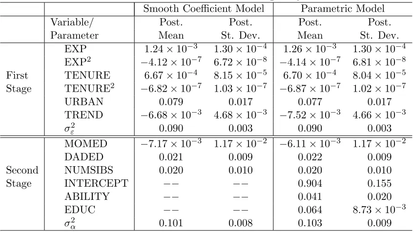
Table 1: Posterior Results for First and Second Stage Parameters: Hierarchical Model Without Endogeneity
Smooth Coefficient Model Parametric Model
Variable/ Post. Post. Post. Post.
Parameter Mean St. Dev. Mean St. Dev.
EXP 1.24×10⁻³ 1.30×10⁻⁴ 1.26×10⁻³ 1.30×10⁻⁴
EXP2 −4.12×10⁻⁷ 6.72×10⁻⁸ −4.14×10⁻⁷ 6.81×10⁻⁸
First TENURE 6.67×10⁻⁴ 8.15×10⁻⁵ 6.70×10⁻⁴ 8.04×10⁻⁵
Stage TENURE2 −6.82×10⁻⁷ 1.03×10⁻⁷ −6.87×10⁻⁷ 1.02×10⁻⁷
URBAN 0.079 0.017 0.077 0.017
TREND −6.68×10⁻³ 4.68×10⁻³ −7.52×10⁻³ 4.66×10⁻³ σε2 0.090 0.003 0.090 0.003 MOMED −7.17×10⁻³ 1.17×10⁻² −6.11×10⁻³ 1.17×10⁻²
DADED 0.021 0.009 0.022 0.009
Second NUMSIBS 0.020 0.010 0.020 0.010
Stage INTERCEPT −− −− 0.904 0.155
ABILITY −− −− 0.041 0.020
EDUC −− −− 0.064 8.73×10⁻³
σ2
α 0.101 0.008 0.103 0.009
Posterior results are produced using the MCMC algorithm described in the appendix.22 A two
di-mensional grid search over values for η1 and η2 indicates support for small values of the smoothing
parameters, and specifically, our empirical Bayesian strategy yields η1 = η2 = 10−12 as the optimal
choice. This indicates that the nonparametric regression lines f1 and f2 are very smooth and can
be taken as informal evidence that a linear model is supported by the data. A more formal test in this regard is provided by the Bayes factor comparing the smooth coefficient model to the parametric model with the mean of the second stage of the hierarchy given by (30). The log of this Bayes factor is
−948.6, indicatingstrong evidence in favor of the parametric model. The reason for this is clear. With very small values of η1 and η2 the two models fit the data roughly equally.23 However, Bayes factors
also have a reward for parsimony built in, and this strongly favors the more parsimonious parametric model (note that the smooth coefficient model has almost 2N more coefficients than the parametric model). This is a general property of our approach and, we feel, a sensible one. Nonparametric mod-els are non-parsimonious, so receive little support unless the parametric alternative fits the data very poorly.
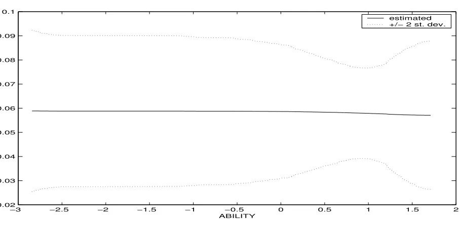
To show the similarity between smooth coefficient results and those from a linear model, Table 1 presents coefficient posterior means and standard deviations from the smooth coefficient and paramet-ric models. For all parameters which are common to both models, it can be seen that the posteriors are virtually identical to one another. In Figures 3 and 4 we present evidence relating to the parameters which are not common to both models and plot estimates off1(A) andf2(A) from the smooth
coeffi-cient model. Figure 3 plots the posterior mean off1(A) (solid) andE(f1(A)|Data)±2Std(f1(A)|Data)
22
We run all MCMC algorithms for 11,000 replications and discard the initial 1,000 as burn-in replications. Our results pass standard convergence diagnostics.
23
(dashed), while Figure 4 similarly plots the posterior mean and posterior standard error bands asso-ciated withf2.
These figures again reveal that the nonparametric and linear models are basically telling the same story. We see some slight nonlinearities in Figure 3, though Figure 3 is not far different from a linear model and results obtained from the linear specification fall comfortably within the plotted standard error bands. From Table 1, the parametric model says that an added year of schooling increases hourly wages by about 6.5 percent with the ±2 Std. interval given by [0.049,0.081]. By construction, the parametric model imposes the same returns to schooling on individuals with different level of ability. Though our flexible smooth coefficient model has the potential of allowing returns to schooling to vary across individuals of differing ability, it estimates the return to education as being roughly constant across individuals of varying ability.24 The smooth coefficient model yields a slightly lower point estimate (roughly six percent), but relative to the size of posterior standard deviations, this difference is negligible. The posterior standard deviations for returns to schooling in the smooth coefficient model are also slightly larger than in the parametric model, which is to be expected given our agnostic stance regarding the specification of the model. Despite these small differences, the parametric and nonparametric models yield roughly the same posterior inferences for returns to schooling and measured cognitive ability.
5.2 Longitudinal Model with Endogeneity
The longitudinal model with endogeneity is given in (16) through (18). The reduced form schooling equation (18) is now added to the analysis. This equation includes an intercept, MOMED, DADED, NUMSIBS, ABILITY and SIBED as explanatory variables, where sibling’s education (SIBED) is the instrument used to identify the model. As in the previous section, we carry along a fully parametric specification and compare results from that specification to those obtained from our smooth coefficient analysis. The first two equations of this parametric model are the same as were used previously in the model without endogeneity. The third equation, (18), is the same in the parametric and smooth coefficient models.
For parameters that are common to both the models in this and the previous section, we retain the same prior specifications that were used in the previous section. We use a noninformative prior for the coefficients in reduced form schooling equation (i.e.,. we set V−1
π = 0 and, with this value, π is
irrelevant). For the prior in (21) we use relatively noninformative values25 of ρ= 9 andA=I2.
24
In a related analysis that did not make use of the nonparametric techniques described here and required time-varying schooling, Koop and Tobias (2002) found little evidence that measured ability played a significant role in explaining variation in returns to schooling across individuals.
25
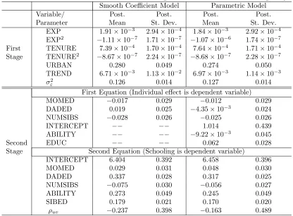
Table 2: Posterior Results for First and Second Stage Parameters: Model with Endogeneity Smooth Coefficient Model Parametric Model
Variable/ Post. Post. Post. Post.
Parameter Mean St. Dev. Mean St. Dev.
EXP 1.91×10⁻³ 2.94×10⁻⁴ 1.84×10⁻³ 2.92×10⁻⁴
EXP2
−1.11×10⁻⁷ 1.71×10⁻⁷ −1.07×10⁻⁶ 1.74×10⁻⁷
First TENURE 7.39×10⁻⁴ 1.70×10⁻⁴ 7.64×10⁻⁴ 1.71×10⁻⁴
Stage TENURE2
−8.67×10⁻⁷ 2.24×10⁻⁷ −8.68×10⁻⁷ 2.28×10⁻⁷
URBAN 0.280 0.049 0.274 0.050
TREND 6.71×10⁻³ 1.13×10⁻² 6.97×10⁻³ 1.14×10⁻³
σ2
ε 0.126 0.014 0.127 0.014
First Equation (Individual effect is dependent variable) MOMED −0.017 0.029 −0.012 0.029 DADED 0.019 0.025 −4.35×10⁻³ 0.024
NUMSIBS −0.028 0.026 −0.025 0.026
INTERCEPT −− −− 1.014 0.439
ABILITY −− −− −9.22×10⁻³ 0.045
Second EDUC −− −− 0.062 0.028
Stage Second Equation (Schooling is dependent variable)
INTERCEPT 6.404 0.392 6.458 0.396
MOMED 0.029 0.031 0.048 0.030
DADED 0.337 0.028 0.317 0.025
NUMSIBS −0.075 0.030 −0.056 0.027 ABILITY 0.273 0.049 0.245 0.049
SIBED 0.179 0.021 0.170 0.020
ρuv −0.237 0.398 −0.163 0.489
We again find little support for the flexibility afforded by the smooth coefficient model for this ap-plication, since empirical Bayesian estimation selects very small values for the smoothing parameters,
η1 = η2 = 10−12. Like the previous section, this result suggests that our semiparametric estimates
will be sufficiently smooth so that simpler parametric models will do an adequate job at reproducing the shapes of the regression curves.
For parameters which are common to both models, we again find that results obtained from the parametric and smooth coefficient models are strikingly similar. The posterior mean (and standard deviation) of the correlation between the errors in two second stage equations (i.e. the source of the endogeneity problem) was found to be −.24 (.40) in the smooth coefficient model and −.16 (.49) in the parametric model. This suggests that with this relatively small sample size26 we are not able to pin down this key correlation parameter, and thus learn little regarding the empirical importance of endogeneity. Finally, it is also worth mentioning that the coefficient on our instrument SIBED is reasonably large in magnitude and clearly “significant” in both the parametric and smooth coefficient models, suggesting it plays an important role in determining the quantity of schooling attained and serves as an adequate instrument.
For those quantities which are not common to both specifications (namely the specification of ability and the ability-education interaction), we found no convincing evidence of nonlinearities.27 This again
suggests that standard parametric models - which are the workhorses of this literature - appear to
26
Recall that we have only 98 individuals to estimate the bivariate relationship in (17) and (18).
27
be adequate for analysis of these issues using the NLSY data. This result both strengthens the conclusions of previous studies which have been based on simpler specifications and also suggests that simpler models are adequate for future work addressing similar topics using the NLSY. We do not view this preference for the simpler model as problematic in any way, but instead are pleased with the fact that our smooth coefficient analysis successfully recreates the findings of a well-fitting parametric model without requiring the assumption of a particular parametric form.
6
Empirical Results: An Ordered Probit Model of Female Labor
Supply
We now turn to our second application involving the NLSY data and model the labor supply decisions of a sample of married white females in 2000. Specifically, we model their decision to remain out of the labor force, to work part time or to work full time in the given year. We estimate our three-choice ordered probit model using the Gibbs sampling algorithm described in the appendix.
In this application we pay particular attention to how changes in spousal income affect changes in our three employment states for women of varying ability. Our smooth coefficient ordered probit model in (26) permits a flexible interaction between ability and spousal income and thus is well-suited for this investigation. As a competing specification we also consider the performance of a fully parametric model that is linear in all the explanatory variables.
Using our empirical Bayesian methods, we settle onη1 = 1.0×10⁻⁷ and η2 = 1.0×10⁻¹¹ as optimal
values of the smoothing parameters. We present in Table 3 below estimation results for the parametric portion of the model using this value ofη1 andη2.
Table 3: Posterior Means and Standard Deviations on Parametric Coefficients
in Ordered Probit Model
Variable Post Mean Post Std.
Num-Kids -.23 .044
Education .033 .027
Unemp-rate .035 .033
Cutpoint (α2) .032 .045
As can be seen from Table 3 (and as one certainly might expect), the number of children in the household plays a strong role in the model, with more children in the home clearly decreasing the probability that a woman works full time and increasing the probability that she remains out of the labor force.
we compute
Pr(y=j|s, w, A=A0, α, γ, θ) = Φ (αj−wθ−f1(A0)−f2(A0)s)−Φ (αj−1−wθ−f1(A0)−f2(A0)s),
where A0 is a particular point in the ability distribution. We set the variables in w equal to their
sample means and evaluate these probabilities at various values of spousal income, s. We calculate these probabilities for each employment state (j = 1,2,3) and for each observed ability valueAi in the
sample. The draws obtained from the posterior distribution ofα,γ and θ, are then used to obtain a point estimate of the desired probability at each ability value. Finally, we also calculate these effects for the competing parametric (linear) specification and compare these estimates to those obtained from the smooth coefficient model.
Results of this exercise are presented in Figures 5 and 6. In these figures we plot results for both the smooth coefficient and parametric models when spousal income is set at $120,000 (approximately the 95th percentile of the spousal income distribution), and thus investigate the impact of ability on female labor supply decisions for those with high levels of family income. As one can see, the figures suggest important differences between the smooth coefficient and linear models. First, the smooth coefficient model suggests that very low ability women are more likely to stay out of the labor force than to work full time at this high level of spousal income. In contrast, the parametric model predicts that the probability of full time work exceeds the probability of no work at all values of the ability distribution. Second, both models suggest that the probability of full time (no) work is increasing (decreasing) with ability, but the slopes of these changes differ considerably across specifications. Specifically, our smooth coefficient model shows a sharp increase in the probability of full time employment for ability values greater than one standard deviation above the mean and a corresponding sharp decrease in the probability of no work over this region. The fully parametric model can not account for these features of the data and simply predicts a nearly linear trend through the ability support.
At the other end of the spousal income distribution, results were very similar across model specifica-tions. When spousal income is $10,000 (approximately the 4th percentile of the income distribution), for example, both the smooth coefficient and linear models predict a high probability of full-time employment and a low probability of remaining out of the labor force regardless of ability level.28 Taken together, these results show there is little evidence of or role for baseline nonlinearities in abil-ity (through f1), but there is an important ability- spousal income interaction (through f2). When
evaluating these probabilities at low levels of spousal income, the contribution of the interaction term is minimal and predictions are found to be similar across the smooth coefficient and parametric models. However, for larger values of spousal income (s), the important role of the ability-income interaction becomes clear. Finally, the log of the Bayes factor in favor of the smooth coefficient model over the parametric alternative was found to be 3.82, indicating preference for the more general smooth coefficient specification despite its added parameterization.
28
We do not present a full set of results for the sake of brevity. Estimates off1,f2 and probabilities of each state with
7
Conclusion
In this paper we have described Bayesian procedures for estimation and testing in cross sectional, longitudinal data and nonlinear smooth coefficient models. In the cross sectional model, estimation, testing and smoothing parameter selection can be carried out analytically, thus making analysis of the smooth coefficient model a simple yet flexible option for practitioners. In the hierarchical smooth coefficient model and nonlinear models that can regarded as linear latent variable models, estimation only requires iterative simulation from standard distributions.
7.1 Appendix A: Posterior Simulator for Longitudinal Model with Endogeneity
The model is given as:
yit = αi+zitδ+εit (31)
αi = wiθ+f1(Ai) +sif2(Ai) +ui (32)
si = riπ+vi, (33)
where again, we let
µi=wiθ+f1(Ai) +sif2(Ai) =xiβ,
as described in section 2.1.
By Bayes Theorem, the joint posterior distribution is proportional to the product of the prior times the likelihood:
p(α, δ, β, π, σ−2
ε ,Σ−1|y, s)∝p(y, s|α, δ, β, π, σ2ε,Σ−1)p(α, δ, β, π, σε−2,Σ−1). (34)
the likelihood function is the joint density of y and the endogenous schooling variable s conditioned on the model parameters. The prior assumptions in (19)-(23) imply:
p(α, δ, β, π, σ−2
ε ,Σ−1) = p(α|β, π,Σ−1)p(δ)p(β)p(π)p(σε−2)p(Σ−1)
=
"N Y
i=1
p(αi|β, π,Σ−1)
#
p(δ)p(β)p(π)p(σ−2
ε )p(Σ−1),
where the last line follows from the assumed conditional independence across observations. The density
p(αi|β, π,Σ−1) can be obtained by substituting out si from (17) using the reduced form equation in
(18).
As for the likelihood function, first let Γ denote all the parameters in the model and note
p(y, s|Γ) =
N
Y
i=1
p(yi1,· · ·, yiTi, si|Γ) (35)
=
N
Y
i=1
ÃT
i
Y
t=1
p(yit|αi, δ, σε−2)
!
p(si|αi, π,Σ−1, β), (36)
where the first line follows by the assumed independence across individuals, and the last equation follows by noting that the density foryitdoes not depend onsi givenαi and thatyit is assumed to be
independent over time givenαi. When appropriate, we have also dropped irrelevant parameters from
the conditioning.
Combining the likelihood in (36) with our prior we obtain the unnormalized joint posterior
p(Γ|y, s)∝
"N Y
i=1
ÃTi Y
t=1
p(yit|αi, δ, σε2)
!
p(si, αi|π,Σ−1, β)
#