An Adaptive estimation scheme for reducing communications in a distributed control implementation

Rochester Institute of Technology

RIT Scholar Works

Theses

Thesis/Dissertation Collections

2-1-2004

An Adaptive estimation scheme for reducing

communications in a distributed control

implementation

Aaron Burry

Follow this and additional works at:

http://scholarworks.rit.edu/theses

This Thesis is brought to you for free and open access by the Thesis/Dissertation Collections at RIT Scholar Works. It has been accepted for inclusion

in Theses by an authorized administrator of RIT Scholar Works. For more information, please contact

[email protected].

Recommended Citation

AN ADAPTIVE ESTIMATION SCHEME FOR REDUCING

COMMUNICATIONS IN A DISTRIBUTED CONTROL

IMPLEMENTATION

By

AARON M. BURRY

A Thesis Submitted to the Faculty of the Rochester Institute of Technology in partial

fulfillment of the requirements for the degree of

MASTER OF SCIENCE

IN

ELECTRICAL ENGINEERING

Approved By

Thesis Advisor

Dr. Mark A. Hopkins

Thesis Committee

Dr. Sohail A. Dianat

Thesis Committee

Dr. Ferat Sahin

Department Head

Dr. Robert J. Bowman

DEPARlMENT OF ELECTRICAL ENGINEERING

COLLEGE OF ENGINEERING

ROCHESTER INSTITUTE OF TECHNOLOGY

ROCHESTER. NEW YORK

AN ADAPTIVE ESTIMATION SCHEME FOR REDUCING

COMMUNICATIONS IN A DISTRIBUTED CONTROL

IMPLEMENTATION

I, Aaron M. Burry, hereby grant pennission to the Wallace Library of the Rochester

Institute of Technology to reproduce my thesis in whole or in part. Any reproduction will

not be for commercial use or profit.

Abstract

This

paperexamines

the

application of adaptive estimation and control

techniques

to

reduce

the

amount of communication required

between

subsystems

in

a

distributed

control

implementation.

Rather

than

require a

large

amount of communications

to

broadcast

the

outputs or

the

states of each of

the

subsystem nodes

to

all of

the

other

nodes at

every sampling

instant,

local

estimators

in

eachsubsystemare used

to

predict

the

state vectors

for

all of

the

other subsystems.

These

estimates are

then

used

in

the

calculation of

the

controller outputs

for

each of

the

subsystems.

Prior

work

in

the

literature has

focused

on static estimation schemes

to

achieve such reductions

in

communications.

However,

such schemes

typically

require

very

accurate models

of

the

plant

in

order

to

maintain

the

desired

reduction

in

communications.

Poorly

modeled

dynamics

or systems whose

dynamics

change

slowly

over

time

(due

to aging

of

components,

changes

in

plant parameters such as a robot

picking up

a

heavy

object,

etc.)

can cause a substantial

increase

in the

amount of communications required

to

maintain

the

desired

system performance.

In

order

to

avoid

this,

this

paper presents an adaptive estimation and control scheme

for

each subsystem

in the

distributed

implementation.

The

stability

of

the

state estimators and

the

convergence of

the

state

tracking

errors

to

withina

desired

threshold

is

proven.

The

performanceof

the

system

using

perfect communication at

every sampling

instant,

using

a static estimation

scheme,

and

using the

proposed adaptive estimation scheme are

then

compared

in

Table

of

Contents

Abstract

i

Table

of

Contents

ii

List

of

Figures

iv

1

Introduction

and

Related Work

1

1.1

Background

. . ... ...

1

1.2

Previous Work

. .

5

1.3

Overview

... . . ... .

8

2

Problem Statement

and

Framework

9

2.1

System

Analysis

. . ....

9

2.2

Problem

Statement

...

18

2.3

Distributed Control Method

... .18

2.4

Adaptive Estimation Method

. . .

20

2.4.1

Estimator Form For

ie(l2

.

21

2.4.2

Estimator Form For

x

G

fi:

24

3

Controller Design

and

Stability

Analysis

25

3.1

No Adaptation

25

3.2

During

Adaptation

. . .

26

3.2.1

Adaptive Controller

26

3.2.2

Adaptive State Estimator

33

4

Performance Metrics

36

4.1

Communication

Metric

36

5

Simulation Results

38

5.1

Spring-Mass-Damper

System

... . ....

39

5.2

Nominal Plant Results

... . .

41

5.3

Effect Of Threshold Values

El0

66

5.4

Comparison Of Results For

Static

and

Adaptive

Estimators

66

6

Conclusions

78

List

of

References

79

List

of

Figures

1

Typical

Distributed

Controller

Implementation

3

2

Totally

Decentralized Controller

Implementation

... .

4

3

Block

Diagram

of

the

State

Estimation Scheme Proposed

in

[1]

7

4

Block Diagram

of

the

ith

Subsystem

In The Partitioned Plant Model

12

5

Partitioned Controller Approach

...

13

6

Block Diagram Of Plant With

Communication

20

7

Block Diagram Of Plant Without Communication

21

8

Trajectory

Of

the

System State Vector

.

32

9

Spring-Mass-Damper

Plant

38

10

State

Tracking

Performance For

Constant Communication

and

Adap

tation:

States

Xi

and

A'2

. . . .43

11

State

Tracking

Performance For Constant Communication

and

Adap

tation:

States

X3

and

X4

44

12

State

Tracking

Performance For Constant Communication

and

Adap

tation:

States

A5

and

A'6

. .

45

13

State Estimator Performance For Constant Communication

and

Adap

tation:

States

Xi

and

X2

...

46

14

State Estimator Performance For Constant Communication

and

Adap

tation:

States

A3

and

X4

47

15

State Estimator Performance For

Constant Communication

and

Adap

tation:

States

X5

and

A6

. .

48

16

State

Tracking

Error

History

For

Constant Communication

and

Adap

tation

50

17

State

Estimator Error

History

For Each

System State

Continuous

Adaptation

51

18

Adaptive

History

of

Controller Parameters

Ki

and

^

Continuous

19

Adaptive

History

of

State Estimator

Parameters

Acj

and

Tjk

Contin

uous

Adaptation

... ...

53

20

State

Tracking

Performance

For

Bounded

Error Adaptation: States

A'i

and

X2

. .

55

21

State

Tracking

Performance

For

Bounded

Error Adaptation:

States

A3

and

A4

.

56

22

State

Tracking

Performance

For

Bounded

Error Adaptation: States

Ar5

and

A6

. . . ...

57

23

State Estimator Performance

For

Bounded

Error Adaptation:

States

Xi

and

A'2

. . .

. . .58

24

State

Estimator

Performance

For Bounded Error Adaptation: States

A'3

and

A'4

. . . ....

59

25

State

Estimator

Performance

For Bounded Error

Adaptation: States

A5

and

Xe

... . .

60

26

State

Tracking

Error

History

For Each System

State

Bounded Error

Adaptation

... .... ... ... .

61

27

State

Estimator Error

History

For Each System

State

-Bounded Error

Adaptation

. . . . ... . .62

28

Communications

History

For Bounded Error

Adaptation

65

29

Effect

of

Changing

the

Error Threshold Parameter

E%0

On System

Tracking

Performance

and

Required

Inter-Subsystem

Communication

67

30

Estimator

Comparison Experiment

. .

68

31

Comparison

of

Tracking

Error Performances For

State

X\

71

32

Comparison

of

Tracking

Error Performances For

State

A2

72

33

Comparison

of

Tracking

Error

Performances For

State

A3

73

34

Comparison

of

Tracking

Error Performances For

State

A4

74

35

Comparison

of

Tracking

Error Performances For

State

X5

75

1

Introduction

and

Related Work

1.1

Background

When

dealing

with

highly

complex

problems,

awell

known

practice

is

to

partition

the

problem

into

smaller,

more manageable pieces.

Each

of

these

pieces can

then

be

analyzed somewhat

independently. The

solution

to these individual

problems can

then

be integrated

together

such

that

a solution

to the

overallproblemcan

be

reached.

There

are

many

other

reasons,

other

than complexity,

for

partitioning

a problem

into

smaller sub-problems

for

analysis.

Resource

allocation,

for

instance,

can

dictate

the

partitioning

of a problem

into

sub-problems which are

then

managed

by

separate

teams.

In

this case, it

is

the

desire

to

have

multiple

teams

analyze portions of

the

problem

in

parallel

that

drives

the

partitioning.

This

type

of

methodology

is

also practiced

in

the

field

of control systems.

The

plant

to

be

controlled

is

partitioned

into

subsystems and

then

separate controllers are

designed

and

implemented

for

each of

these

subsystems.

This

strategy

is

referred

to

as

distributed

control.

In

centralized controller

implementations,

all of

the

required

sig

nals

(feedback

from

output

sensors,

state

feedback

signals,

and reference

inputs)

are

routed

to

a single

location.

The

controller

is

designed

based

on

full knowledge

of

the

required signals and

implemented

at

the

central

location

where

these

signals

have been

routed.

In

contrast,

a

distributed

control

implementation

places

the

decision-making

and computation of

the

controller

into

the

subsystems

themselves.

In

addition,

in

a

distributed

control

implementation the

local

subsystem controllers

typically

do

not

have

access

to

all of

the

outputs nor all of

the

states of

the

other subsystems at each

sampling instant.

This

means

that

the

subsystemcontrollers must

base

their

decision

making

and control actions on a more

limited

set of

information

than

in

acentralized

implementation.

The

amount of non-local

information

required

by

each subsystem

controller

is determined

by

a

variety

of

factors,

including: the

dynamics

of

the plant,

the

chosen

partitioning

of

the

plant

into

subsystems,

and

the

design

of

the

subsystem

achieve

the

desired

system performance

is

part of

the

design

of a

distributed

control

system.

The

amount of communication at each

sampling

instant

that

is

supported

by

the

implementation

can

vary

from full

stateor outputcommunication

(essentially

cen

tralized

control

implemented

over a communications

network)

to

no communication

at all

(totally

decentralized

control).

A block

diagram

of a

typical

distributed

controller

implementation

is

presented

in

Figure

1.

In

this

figure,

the

plant

has been

partitioned

into

n subsystems where

the

H;

are

the

subsystem

controllers, the

xl

the

local

subsystem state

vectors,

and

the rt

are

the

reference

inputs

to

each of

the

subsystems.

In

this scheme,

a communications

bus

(the

control

network)

has been

provided

to

enable

the

exchange of

information

between

subsystems.

The

required amount of communication at each

sampling

in

stant,

or perhaps

the

maximum amount

if the

rate of exchange

varies,

would

then

dictate

the

required

bandwidth for

this

communications channel.

Figure 2 illustrates

an extreme example where

the

subsystem controllers

only

have

access

to the

local

state vector and reference

input,

providing

no mechanism

for information

exchange

between

subsystems.

This

type

of configuration

is

known

as

totally

decentralized

control.

Distributed

control can offer a

variety

of advantages over a centralized scheme.

These include

[2]:

taking

advantage of

the

distribution inherent in

some

plants;

in

creased

processing capability

due

to the

increase

in the

number of compute engines

(typically

one per

subsystem);

flexibility

to

changes

in

the plant;

improved

tolerance

to

failures in

parts of

the system; enabling

controllers

to

be

delivered

as part of

their

associated

subsystems;

and possible advantages

in

cost

due

to

reduced wiring.

When

designing

a

distributed

control

system,

it is obviously necessary

to

guaran

tee

the

overall

stability

of

the

system and

that

the

desired

performance objectives are

achieved.

One

factor

that

can

strongly influence

both

the

stability

and performance

of

the

system

is

the

amount of physical

coupling

between

subsystems

in

the

plant.

If

n,

ui

Plant

xi

Ut

n:

X,

Un

n

xn

Communications

Bus

Figure

1:

Typical Distributed Controller Implementation

interactions

can

lead

to

significant performance

degradations, instability

in the

sys

tem,

or even system

failures. The

reason

for

this

is

that

each

distributed

subsystem

controller

is

acting

upon a reduced set of

information

when

calculating its

control

output

to the

plant

(an

extreme example of

this

can

be

seen

in

Figure 2

where

there

is

only

feedback

of

the

local

state

information).

Strong

coupling

in

the

plant

between

subsystems means

that

non-local

behavior in

the

system

is

impacting

the

evolution

of

the

local

subsystem states.

In

essence, these

unknown

coupling interactions

are

acting

as

disturbances

to the

local

subsystems.

If

the

design

of

the

local

controllers

is

not

sufficiently

robust

to

these

disturbances,

the

coupling interactions

can

lead

to

instability

of

the

system.

Thus,

the

design

of

the

subsystem controllers and

the

communications mechanism must somehow account

for

these

coupling interactions in

order

to

guarantee

both desired

performance and system stability.

The

robustness of

the

communications channel

in

a

distributed

control

imple

mentation can also

impact both

system

stability

and performance.

Message

packet

delays,

lost

messages,

and other communicationsrelated problems can

impact

the

re

n,

u,

Plant r.

xi

u,

n2

r.

X,

11n

n

n

rn

\,

Figure

2:

Totally

Decentralized Controller Implementation

with

faulty

and/or out-of-date

information

can result

in inappropriate

controlactions.

These

undesirable controller outputs can

then

lead

to

poor performance or even

in

stability

of

the

system.

In

many cases, requiring the

exchange of

large

amounts of

information between

subsystems at each

sampling

instant

can contribute

to these

types

ofproblems.

Unexpected

message packet

delays

in

particular can

be

caused

by

over-burdening

of

the

communications network.

So

it is

important to

ensure

that the

communication network

is

capable of

sup

porting the

required

level

of

information

exchange

between

subsystems.

However,

the

higher

the

bandwidth

of

the

communications

channel, the

more

costly

the

im

plementation will

usually

become.

This

means

that there

is

typically

a

strong desire

to

minimize

the

required amount of communications

between

subsystems while still

achieving

acceptable system performance.

A

further

complication

is

that the

amount

of

information that

must

be

exchanged

between

subsystems can

vary

from

sampling

instant

to sampling

instant based

on a

variety

of

factors.

Thus,

it is

typically

difficult

1.2

Previous

Work

A variety

of methods

have been

presented

in

the

literature

for

guaranteeing

system

stability

and performance while still

requiring

a

limited

communications

bandwidth

between

subsystems

in

a

distributed

control

implementation. These

methods can

be

separated

into

two

basic

types

of approaches.

The

first

type

of approach

involves

developing

analysis and

implementation

techniques to

minimize

the possibility

of

system

failures

due

to

communication

issues.

The

goal of

this type

of approach

it

to

enable

the

implementation

of a

lower

bandwidth

but

more reliable communications

channel

between

subsystems.

One

such approach

is

outlined

in

[3]

where

the

authors

have focused

on

analyzing the

real-time communications requirements and constraints

in

an effort

to

better

predict system reliability.

The

goal

is

to

predict

in

advance

the

capability

of

the

network

to

support

the

information

exchanges required and

the

probability

of potential

failures.

In

[2]

the

controller

is

designed

assuming

a centralized

implementation.

The

actual

distributed implementation

then

requires

information

exchange

between

subsystems

across a network.

The

authors propose a mathematical

framework

for analyzing

the

performance

degradation

of

the

controllers

due

to

communication

delays in

the

network.

An

analysis

technique

for

defining

an upper

limit

on

the

allowable communication

interval in

a networked control system while still

guaranteeing

stability is

presented

in

[4].

The

authors assume

that the

distributed

nodes must communicate

their

out

puts

to

one another.

An

extension of

this

result

is

presented

in

[5]

where a prediction

method

is

used

to

predict

the

output of each subsystem

between

consecutive

transmis

sions of

the

actual outputs.

This

allows

for

an extension of

the

maximum allowable

delay

between

output

transmissions

while still

guaranteeing

system stability.

Other

authors

have

taken

a

slightly

different

approach

attempting

to

limit

the

amount of communications

that

are required

between

subsystems as part of

the

dis

allowing

any

information

exchange

between

subsystems at all

(totally

decentralized

control).

Many

authors

have

developed

techniques

for

designing

subsystem controllers

that

are robust

to the

interactions

between

subsystems.

Approaches

such as

[6], [7],

[8], [9],

and

[10]

all

involve

designing

distributed

controllers

that

do

not require

any

information

exchange

between

subsystem nodes while still

achieving

acceptable sys

tem

performance.

These

approaches make use of an adaptive process

to

make

the

localized

controllers robust

to the

coupling

between

subsystems.

In

each

case, there

are restrictions placed on

the

plant

dynamics,

the

size of

the

interactions,

or

both

in

order

to

guarantee stability.

In

[1]

an approach

is

outlined

for

minimizing

(rather

than

eliminating)

the

com

munications

between

subsystem nodes

in

a

distributed

control

implementation.

This

is

accomplished

by

using

state estimation at each node

in

the

system

to

predict

the

state vectors of

the

other subsystems.

In

this way, the

state

information

for

each

node

does

not

have

to

be

communicated

to

all other nodes at each

sampling instant.

Instead,

each controller uses estimated values of

the

state vectors

for

the

other nodes

in

the

system

to

update

its

control vector at each

sampling instant.

Figure 3

shows

a

block diagram

of

this

approach.

In

this

figure,

the

region enclosed

by

the

dotted

square

is

an

internal

view of subsystem

1.

Each

of

the

other subsystems would

have

a similar structure.

So

each subsystemcontains an

implementation

of

the

full

system

controllerand a

full

system estimator.

The

estimated outputs are used

in

conjunction

with

the

locally

measurable outputs

to

determine

the

local

controller output

to the

plant.

In

order

to

guarantee acceptable

tracking

using this approach, the

authors

enforce an upper

bound

on

the

state estimation error

for

each node's state vector.

When

the

state estimation error

for

the

ith

node

is larger

than this

pre-established

bound,

the

locally

measured system outputs

for

this

node are communicated across

the

bus

to

all

the

other nodes

in

the

system.

The

other nodes can

then

use

the true

output vector

for

the

ith

node

to

update

the

states of

their

local

estimators.

The

Controller

1

'full

Controller

(full sys)

Estimator (full sys)

IS

Subsystem 2

Subsystem 1

'M

Subsystem M

JM

yM

[image:16.505.85.423.48.299.2]

Plant

Figure 3: Block Diagram

of

the

State Estimation

Scheme

Proposed

in

[1]

performance of

the

system

to

be

traded

off against

the

amount of communications

traffic

required

between

subsystems.

The

success with which

this type

of approach can reduce

the

required rate of com

munications

between

subsystems

is

highly

dependent

upon

the

accuracy

of

the

plant

model used

in the

design

of

the

state estimator.

Along

these

lines,

an

issue

that

is

not

addressed

by

this type

of approach

is

the

effect of

slowly

changing

plant

dynamics.

Take

the

case of a plant whose

dynamics

are affected

by

frictional

wear or other age

related effects

to

its

mechanical elements.

Using

the

static state estimation scheme of

[1],

the accuracy

with which

the

original state estimator represents

the

actual plant

would

slowly

decay

over

time

as

the

plant

dynamics

evolve.

Without

some

form

of

re-tuning

of

the

state estimator

being

used, this

degradation in

the

performanceof

the

state estimator would result

in

a growth

in

the

amount of communications required

between

subsystems over

time.

In

extreme

cases, this

could result

in

communications

1.3

Overview

The

objectiveof

this

work was

to

develop

an adaptive control scheme

that

could

be

used

to

reduce network message

traffic

in

a

distributed

control

implementation

while still

achieving

acceptable state

tracking

performance and

guaranteeing

overall system stability.

An important

goal of

this

work was

to

demonstrate

improved

performance

of

this

adaptive method over a static estimation and control scheme

for

the

case of

poorly

modeled plant

dynamics.

The

remainder of

this

paper

is

organized as

follows: The framework

of

the

prob

lem

and an analysis of

the

system

dynamics is

presented

in Section

2;

The

stability

of

the

overall system as well as

the

convergence of

the

tracking

error

during

adapta

tion

is

proven

in

Section

3;

Simulation

results

demonstrating

the

performance of

the

2

Problem Statement

and

Framework

2.1

System Analysis

Consider

an

M

input,

M

output plant

described

by

the

following

equations:

x{t)

=

Ax(t)

+

Bu(t)

+

Br(t)

(2.1)

y{t)

=

Cx{t)

(2.2)

where

x(t)

E

$tN

is

the

state vector of

the plant,

u(t)

e

5?M

is

the

control

vector,

r(t)

G

5RA/

is

the

vector ofreference

inputs

to the system,

and

y(t)

G

UM

is

the

output

vector.

The

matrices

A, B,

C

are,

for

the moment,

assumed

to

be

constant and of

the

following

sizes:

A

:

N

x

N,

B

:

N

x

71/,

C

:

M

x

N

In

this

investigation it is

assumed

that the

B

and

C

matrices are

known,

but

that

the

A

matrix

is

unknown.

Now,

the

plant

is

partitioned

into

M

coupled subsystems where each subsystem

is

single-input.

After

the partitioning,

each subsystem

has

Np

states where

N

=

MNp.

It is

assumed

that the

system

has

been instrumented

such

that

all of

the

states of

the

local

subsystems are measurable.

Furthermore,

for

the

purposes of

this

investigation,

only

those

plants whose

input

and output matrices are

in

the

following

form

are considered:

B

=

blkdiag(Bu

B2,...

BM)

(2.3)

C

=

where

the

Bt

are vectors of size

(Np

x

1)

and

the

C;

are vectors ofsize

(1

x

Np).

A

system composed of

interconnected

masses,

such as

the

spring-mass-damper

system presented

in

Section

5.1,

is

an example of a system

that

satisfies

these

re

quirements.

In

this example, the

system

is

partitioned such

that the

subsystem state

equations

describe

the

dynamics

of each of

the individual

masses.

There is

aseparate

force input

applied

to

each of

the

masses

that

does

not

directly

affect

the

motion of

the

other masses

in

the

system

-the

applied

force

only

directly

affects

the

acceleration

of

the

mass while

the

coupling between

the

masses occurs

through

the

positions and

velocities.

Because

the

subsystem

interactions

occur

through

states of

the

system

that

are not

directly

affected

by

the

subsystem

inputs,

the

input B

matrix will

be

of

the

desired block diagonal form.

Assuming

that the input

matrix

is block

diagonal,

the

state

dynamics

of

(2.1)

can

be

rewritten as

follows:

B1

0

0

B2

0

0

xx

2

0

0

An

Ai2

A2\

A22

Aim

A2m

B

M

A

U-2

UM

Ml

AMl

' - '

Si

0

0

B2

0

0

A

MM

Xl

X2

Xm

+

0

0

B

M

r2

rM

(2.5)

where

An

is

the

Np

x

Np

matrix

representing the

local

state

dynamics

of

the

zth

subsystem,

A^-

is

the

Np

x

Np

matrix

representing the

coupling

dynamics

between

the

states of

the

zth and

jth

subsystems,

xt

is

the

Np

x

1

state vector of

the

ith

subsystem,

5;

is

the

Nv

x

1 input

matrix of

the ith. subsystem, r;

is

the

1

x

1

reference

Factoring

the

interaction

terms

from

the

A

matrix

in

(2.5),

the

following

is

obtained:

Xl

x2

xm

An

0

0

A22

0

0

0

Al2

A21

0

Ami

Am2

0

0

A

_MM ''1

X2

xM

+

5i

0

0

B2

0

0

0

Ui

0

u2

Bm

Um

+

A\M

A2M

Xl

x2

xm

+

Bi

0

0

B2

0

0

0

0

B

M

Tl

r2

(2.6)

This

expression can

be

simplified

by

writing,

Xl

2

xM

Mi

0 0

A22

0 0 X2 XM

Si

o 0 0 0

("i +n)

01

("2 +r2)

+

4>2

(M

+ rAI)

4>M

(2.7)

where,

A/ M

>>2

=

Y.

AVX3

M

9j

/ j

/iij Xj

j=l,j^ti

(2.8)

Here

the

fa

matrices represent

the

contribution

to the

state

dynamics

of

the

z'th

subsystem

due

to the

other

(M

1)

subsystems.

The

dynamics

of

the

zth subsystem

can now

be

written:

i(t)

=

AiXiit)

+

BiUi(t)

+

BiTi(t)

+

fa

yi(t)

=

where,

i

=

1,

2,

. . .

,

M,

xt(t)

G

^RNp

is

the

state vector of

the ith subsystem,

Az

=

Au,

Ui(t)

G

5R1

is

the

controller output

for

the

ith

subsystem,

r,(t)

G

3?1

is

the

reference

input

for

the

ith

subsystem,

and

yl(t)

G

5ft1

is

the

output of

the

ith

subsystem.

A

block

diagram

of

this

subsystem model

is

shown

in

Figure

4.

U.

<f>,

Figure

4:

Block Diagram

of

the ith

Subsystem

In The Partitioned Plant Model

The

objective

is

to

design

a controller

n

that

will

force

the

states of

(2.1)

to track

those

of

the

following

reference model:

xm(t)

=

Amxm(t)

+

Br(t)

(2.10)

assumed

to

be

completely

decoupled

such

that,

Ar

Ami

0

0

0

Am2

0

0

0

A

mM

(2.11)

If

the

reference model

in

(2.10)

is

then

partitioned

into 71/

subsystems,

the

dynamics

of

the

ith

subsystem of

the

reference model can

be

written

as,

xmi(t)

=

Amixmi(t)

+

Bir^t)

(2.12)

The

objective

is

then to

design

the

subsystem controllers

(nA

that

will

force

the

subsystem states

re*

to track the

reference model statesxmi.

A diagram

of

the

proposed

system

partitioning is

shown

in

Figure

5.

In

this

diagram,

it is

assumed

that

a

communications

bus is

available

to

enable some amount of

information

exchange

between

subsystems.

Part

of

the

design

of

the

subsystem controllers

Hj

is

determining

how

much

information

will need

to

be

communicated across

this

bus.

n,

n

;

fc

nn

ffliU

>

Communications Bus

xl

u.

X,

Un

-_ Xn

In

order

to

ensure

that the

controller

for

the

ith

subsystemcancompensate

for

the

interaction

terms

(fa)

in

(2.7),

a restriction of

the

form

posed

in

[10]

will

be

adhered

to.

This

restriction requires

that the

interconnection

terms

be

representable

in the

following

form:

71/

&=

B^Xj

(2.13)

where

the

Ax

1

vector

^

represents

the

unknown

linear coupling between

subsystems

i

and

j.

A

comparison of

this

equation with

(2.8)

shows

that this

restriction equates

to the

following,

Aij

=

B^l

(2.14)

The

nature of

this

restriction can

be better

understood

in

the

context of

(2.6).

From

this equation, the

dynamics

of

the

ith

subsystem

are,

xz

=

B{r{

+

BiUi

+

AaXi

+

[Anx1

+

Ai2x2

+

. .

+

AiNxN]

(2.15)

where

the term

AtiXi

has been

intentionally

moved outside

the

brackets. The

restric

tion

in

(2.14)

requires

that the

equation above can

be

written as

follows:

xz

=

Bxri

+

B^i

+

AaXi

+

Bt

[V^Zi

+

ip[2x2

+

+

iP[nxn]

(2.16)

A

comparison of

(2.15)

and

(2.16)

shows

that

imposing

this

constraint amounts

to

reducing the complexity

of

the interaction terms.

Specifically,

the

contribution

from

the

jth subsystem

to the

dynamics

of

any

of

the

other subsystems

is simply

aweighted

linear

combination of

the

elements of state vector Xj.

The

extent

to

which

this

scalar

quantity

(tjjfjXj)

affects

the

evolution of each of

the

states

in

subsystem state vector

Xi

is determined

by

the

local input

vector

Bt.

Thus,

the

contributions

to

each element

of

Xj

from

Xj

are not

linearly

independent

as

they

are

for

(2.15).

This

is

the

reduction

in

complexity

of

the

interaction

terms that

wasreferred

to

above.

An

example system

The

reason

for enforcing

the

restriction

in

(2.14)

is

to

ensure

that the

controller

for

the

ith

subsystem

is

capable of

fully

compensating

for

the

contributions

from

the

other

(M

1)

subsystems.

The

goal would

be

to

have

a

term

in

the

controller

act

to

completely decouple

the

ith

subsystem

from

the

dynamics

of all of

the

other

subsystems.

Substituting

(2.13)

into

(2.7),

the

dynamics

_of

the

ith

subsystem can

be

represented

in

the

following

form:

M

Xi(t)

=

AiXi(t)

+

BiUi(t)

+

Bitiit)

+

Bt

ipfjXj

i=ij/z

Vi(t)

=

Qx^t)

(2.17)

where

i

=

1,2,...,

M.

From

this

equation

it is

clear

that,

if the ith

controller

has

perfect

knowledge

of

the

states

Xj

of

the

other

subsystems,

then

a controller

term

of

the

following form,

M

Ut

=

-J2

^HXJ

(2-18)

allows

the

controller

to completely

decouple

the

state

dynamics

of

the

ith

node

from

those

of

the

other subsystems when

ip^

= _ip^.

Other

terms in the

_{controller could}

then

be

utilized

to

ensure

that the

subsystem states

Xj

track those

of

the

desired

reference model xmi.

Using

a controller

form

similar

to that

presented

in

[6],

the

control vector of

the

ith

subsystem

(ut)

is designed

as

follows:

M

Ui

=

Kjxi-Y.

$jxo

(2-19)

where

ipij

G $lNp

is

the

estimation of

the

unknown

coupling

between

the

ith

and

jth

subsystems and

Ki

is

the

local

state

feedback

controller gain vector.

The

second

term

in

this

controller equation acts

to

decouple

the

dynamics

of

the

ith

subsystem

from

the

rest of

the

system.

The

state

feedback

term

K?Xi

then

serves

to

adjust

the

Substitution

of

(2.19)

into

(2.17)

gives

the

following

model

for

the

ith

subsystem:

M M

i(t)

=

AiXi(t)

+

Bi[kfxi(t)-

Y

tfjxA

+

BinW

+

Bi

Y

^lxi

yx(t)

=

dxi(t)

(2.20)

In

order

to

guarantee

that

a controllerof

the

form

posed

in

(2.19)

can

successfully

achieve

the

desired

tracking

objective,

another

important

restrictionmust

be

imposed.

This

restriction

is

that,

for

some unknown controller gain vector

K*,

the

following

relation must

hold:

Ami

=

A

+

BxKf

(2.21)

Rearranging

this

equation

slightly

will

help

with an

intuitive

understanding

of

this

restriction.

Ami

-Ax =

B{Kf

(2.22)

Here it is

clearly

seen

that the

imposed

constraint places a restriction on

the

difference

between

the

desired

system

dynamics

(those

of

the

reference model

Ami)

and

the

nominal plant

dynamics

(AA. Once

again, this

will ensure

that the

proposed controller will

be

capable of

achieving the

desired

tracking

objective.

A

more

fundamental

understanding

of

the

reason

for

imposing

this

constraint can

easily

be

obtained

by

close

inspection

of

(2.20).

If

the

estimates of

the

interaction

terms perfectly

match

the

actual

coupling

dynamics

then,

4>a

=

4>ij

(2.23)

and

(2.20)

can

be

reduced

to the

following:

i(t)

=

[Ai

+

BikJ]xi(t)

+

Bin(t)

Vi(t)

=

A

comparison of

this

equation with

(2.12)

clearly

shows

that

perfect

tracking

of

the

reference model states

is

guaranteed

if

(2.21)

holds

and

Kt

=

K*.

Since

this

desired feedback

gain vector

is

assumed

to

be

unknown, the

problem

then

becomes

designing

the

appropriate

local

feedback

gain vectors

Kx

that

will ensure

tracking

of

the

reference model states.

A

closer

inspection

of

the

restriction

imposed

by

(2.21)

is

now

in

order.

A

sufficient

condition

for

this

restriction

to

be

satisfied

is

that

both

the

reference model

dynamics

and

the

subsystem

dynamics

be

expressible

in

the

following

companion

form

(the

idea

of

expressing

the

subsystems of

the

reference model and

the

plant

in

this

form

is

borrowed

from

Gavel

and

Siljak

in

[10]):

A,

0

0

~oA

(fc-i)

-a

1

0

(fc-2)

-a

0

1

(fc-3)

0

0

-a]

Ai

=

0

0

1

0

0

1

~P\k-l)

~P\k-2)

P[k-Z)

0

0

-PI

(2.25)

Bx

=

Bmi

=

[

0

0

. .

0

1

]

Ci

=

Cmi

=

1

₀

₀

...

0

If

the

system and

the

reference model can

be

expressed

in

this

general

form

then,

(Ar

AA

=

0

0

0

0

0

0

(%-d-4-d)

(fl

(fc-2)

a\k-2))

(PI

-<*[)

From

this

equation and

the

form

of

Bt

in

(2.25)

it is

clear

that,

3K:\Ami

=

Ai

+

BiK;T,\/i

(2.27)

and

(2.21)

is

satisfied.

In

fact,

this

desired

gain vector

is

given

by,

A'M ($*-!)

-<Vd)

(%-2)-^fc-2))

(/3i-i)f

(2-28)

This

analysis

has

shown

that

if

the

subsystem

dynamics

can

be

written

in

the

companion

form

of

(2.25),

then the

restriction

imposed in

(2.21)

will

be

satisfied.

While

the

companion

form is

not required

to satisfy this restriction,

it is

a sufficient

condition.

Further,

a sufficient condition

for

the

system

to

be

expressible

in

the

proposed companion

form is

that the

subsystems

be both

controllable and observable

[10].

Thus,

a sufficient condition

for

the

restriction

in

(2.21)

to

be

met

is

that the

system

being

analyzed

is

both

controllable and observable.

2.2

Problem Statement

With

the necessary

constraints on

the

plant

dynamics

satisfied, the

problem

is

then to

design

the

subsystem controller gains

Ki

and

the

estimates of

the

interaction

terms

ipij

in

(2.19)

for

each of

the

71/

subsystems,

such

that the

plant states

Xj

track

those

of

the

reference model xmi.

It is

further

required

that the

design

of

the

subsystem controllers provide a mechanism

for

reducing the

amount of

inter-node

communications,

while still

guaranteeing stability

and

achieving

the

desired

tracking

performance.

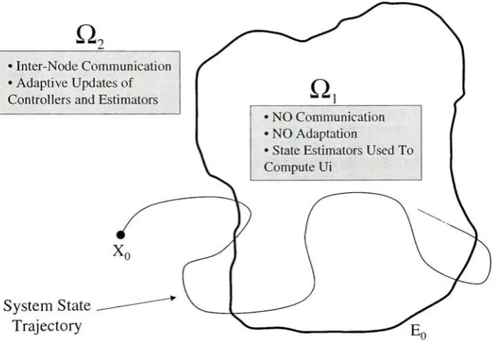
2.3

Distributed Control Method

The

controller

form

proposed

in

(2.19)

requires

that the

ith

subsystem

have

com

plete

knowledge

of

the

state vectors of

the

other

(M

1)

subsystems

(the

Xj

terms

in

this

equation).

This is

equivalent

to

a centralized controller

implementation

and

the

other

(71/

1)

subsystem at each

sampling

instant.

In

many cases, implementa

tion

constraints

(such

as

limited

communication

bandwidth)

make

this

requirement

impractical. In

order

to

limit

the

amountof communication required

between

subsys

tems,

a state estimation scheme will

be implemented

at each node.

These

estimators

will predict

the

states of

the

other nodes

in the

system.

The

subsystem controllers

can

then

use

the

output of

these

estimators

to

calculate

their

control

actions,

rather

than

requiring

the

actual states of

the

other subsystems.

As

long

as

the

estimator

outputs are used

in

the

subsystem

calculations,

no communication

between

subsys

tems

is

required.

With

this

estimation scheme

in

mind, the

control vector

for

the

ith

subsystem needs

to

be

modified

from

the

form

shown

in

(2.19).

Define

the

state

tracking

error

for

the

ith

subsystem node as

follows,

Cj

Xi

xm^

^z.zyj

Now,

the

state space of

the

system

is

partitioned

into

two

regions as

follows:

x

G

Q\

:

efe* <

El0,Vi

x

G

Q2

:

3z

]

ejei >

El0

(2.30)

where

El0

is

the

desired

performance

bound

for

the ith

subsystem.

The

controller

output will

then

be different for

each of

these two

regions.

Using

a

bounded

error

approach similar

to that

presented

in

[1]

and

[11],

the

controller

for

the

ith

subsystem

is

defined

as,

u =

[

ft*

-E&,,-*

$*;

fOT

**

i

,2 311

1

\

kJxi-^U^i^j

forxGQ2

where

Xj

G

3tNp

is

the

estimated state vector

for

the

jth subsystem.

Thus,

the

estimated states of

the

other

(M

1)

subsystems are used

to

determine

the

control

xl

II,

Plant

. Xl

ul

r(ull

*1'X3

^n

x2

n

₂ X-,

r.uii

u2

xx2,."..,xn

*n

n

, v"

rfull

Un

nications

Bus

Figure

6:

Block Diagram Of Plant With Communication

(efet

<

ElQ).

A block diagram

of

the

system under

these

conditions

is

presented

in

Figure

7.

Once

the

tracking

error grows

beyond

this

bound,

the

actual subsystem

states will

be

communicated

between

nodes and used

to

determine

the

controller

output

Ui

at each node

(see

Figure 6).

The design

of

the

controller and estimator

parameters

to

ensure

stability

and

desired

tracking

performance

using

this

scheme

will

be investigated in Section 3. Section 2.4 describes

the

proposed method

for

each

node

to

estimate

the

state vectors of

the

other nodes

in

the

system.

2.4

Adaptive

Estimation Method

One

of

the

key

features

of

the

present approach

is

the

use of an adaptive state

estimator

to

reduce

the

amount ofcommunicationsrequired

between

subsystems while

still

maintaining

acceptable

tracking

of

the

reference model states and

guaranteeing

system stability.

Rather

than requiring that

each subsystem node communicate

its

statevector

to

all of

the

other

(M

1)

nodes at each

sampling

instant,

each node uses [image:29.505.112.390.63.276.2]

r

_, Local State Estimator A

X

II,

x

Plant

r IIIII

Un

X

xn

Local State Estimator

n2

rfull

_,

riull

Un

'

X

*

Local State Estimator

rt

u1 1

nn

rfull

U

Figure

7:

Block

Diagram

Of Plant

Without Communication

state values are

then

used

by

each node

to

calculate

the

required

local

controller

output

to

achieve

the

desired

tracking

performance.

There

are

two

separate

forms for

the

proposed state estimator

that

need

to

be

considered one

for

each of

the

state space regions

defined in

(2.30).

Each

of

these

forms

will

be

considered

separately below.

2.4.1

Estimator Form For

x

G

fi2

Recall

that

full

knowledge

of

the

system states

is

assumed when x

EVt2.

As

long

as

the

state vector remains

in

this region,

communication

between

subsystems will

occur and

the

adaptive process will adjust

the

controller and estimator parameters.

For

this situation, the

state

dynamics for

the jth.

subsystem node are as

follows:

M M

Xj

=

AjXj+Bj[kJxj-Y ^kxk]

+

Bjrj

+

Bj

Y

tfkxk

k=l,k^tj

fc=l,fc^j

Define

the

local

closed

loop

state

dynamics, ignoring

the coupling

interactions,

for

the

jfth node

to

be,

ACJ

=

A,

+

BjKj

(2.33)

Ignoring

the

interactions

between

subsystems

in

(2.32),

the

following

state estimator

is

then

proposed

[12]:

%

=

AmjXj

+

(Acj

-Amj)Xj

+

B]r]

(2.34)

This

estimator

form

requires

knowledge

of

the

subsystem states

Xj

that

it is

trying

to

estimate.

The

purpose of

this

form is

to train the

estimator while

the

actual state

values are available.

Once

the

parameters of

the

estimator

have been

sufficiently

adapted, then the

estimates of

the

states can

be

used

in

place of

their

actual values.

Now,

for

the ith

node

(j ^ i)

the

actual state values

Xj

are

only

available when

there

is

communication

between

the

ith

and

jth

nodes

(when

x

G

Cl2).

Once

the

system state vector enters region

f2i,

inter-subsystem

communication will cease and

the

actual state values

Xj

will no

longer be

available.

Thus,

the

form

of

the

estimator

will need

to

be

modified

to

account

for

this.

This is discussed

in

Section

2.4.2.

The

motivation

for

choosing the

estimator

form

in

(2.35)

becomes

clearer after

a minor manipulation of

this

equation.

Using

the

fact

that

ACj

ACj

ACj

this

equation can

be

rewritten

as,

Xj

-rijjijXj "r/\qjX

j

"r -<*cjXj \

X^j'j

yZ.ooj

Now,

for

the

case where

the

output of

the

state estimator converges

to the

actual

state vector

Xj, then

Xj

>

0.

Further,

if

the

model

for

the

local

state

dynamics

ACj

converges

to that

of

the

actual

dynamics

ACj,

then

Acj

>

₀

as well.

Under

these circumstances, the

first

and

third terms

in

(2.35)

are zero and we are

left

with

Xj

=

ACjXj.

This is

is

trying

to

predict.

Thus,

if

the

adaptive process can

drive

the

state estimation error

Xj

and

the

modeling

error

Acj

to zero,

(2.35)

provides

the

appropriate

form for

the

estimator

dynamics.

The

estimator

form in

(2.35)

does

not account

for

the interactions

between

sub

systems.

However,

these terms

cannot

be

neglected

in

the

actual

system,

so

the

form

of

this

equation must

be

modified

to

account

for

this.

The form

of

the

estimator

could

be

chosen

as,

M

Xj

=

AmjXj

+

(Acj

-Amj)xj

+

BjTj

+

B3

Y

^lkxk

(2-36)

k=l,k^j

where,

ipjk

=

ipjk

ipjk

represents

the

error

in

estimating the interactions

between

nodes

j

and

k.

Unfortunately,

this

form

requires

that the

actual values of

the

esti

mation error

ipjk

be known.

Since

the

actual

interaction

terms

ipjk

are assumed

to

be

unknown, this

is

not a realistic requirement.

Thus,

a slight modification needs

to

be

made

to

(2.36).

Define

the

following:

Tj-fc

=

ipjk

(2.37)

The form

of

the

adaptive state estimator

is

then

be

written as

follows:

M

ij

=

Amjxj

+

(Acj

-Amj)xj

+

Bjrj

+

Bj

Y

^Jkxk

(2.38)

k=l,kjj

where,

Tjk

=

ipjk

is

the

actual error

in modeling the coupling

between

nodes

j

and

k

and

Fjk

represents

the

estimate of

this

error

term.

Thus,

since

the

actual

ipjk

vector

is

not available

for

measurement, this quantity

will

be

estimated.

The

choice ofadaptive

2.4.2

Estimator

Form For

x

G

fii

While

the

system state vector

is

within region

Jli,

communication

between

subsys

tems

does

not occur.

Thus,

the

actual state vectors

x3

and

xfc

in

(2.38)

are no

longer

available

to the

ith

subsystem.

Under

these circumstances, the

proposed estimator

form

needs

to

be

modified slightly.

In

particular, the

estimates of

these

states will

be

used

instead

of

their

actual values.

Temporarily

ignoring

the coupling interactions

between

subsystems and

substituting

Xj

=

j

in

(2.34)

then

produces

the

following,

'j

AcjXj

+

BjXj

(2.39)

Thus,

when x

G

Q\

the

estimate of

the

closed

loop

dynamics

of

the jth

subsys

tem

(ACj)

determines how

the

estimated state vector

Xj

will evolve.

For

the

more

general case

that

includes

the

contribution

from

the coupling

between

subsystems,

substituting

Xj

=

Xj

and

xk

=

xk

in

(2.38)

produces,

M

=

AC3x3+BJrJ

+

B]

Y

Fjkxk

(2.40)

k=l,k^j

This is

the

form

of

the

state estimator

that

will

be

utilizedwhen x

G

f^i- No

adapta

tion

of

the

estimator parameters occurs while

the

system state vector remains within

this

region.

It is

assumed

that

the

estimator

is

providing sufficiently

accurate

results,

so

long

as

the

tracking

error

for

all of

the

subsystems remains

below

the

desired

thresholds.

If

the

tracking

error

for

any

of

the

subsystems grows

beyond

its

threshold

(El),

then

communication

between

subsystems and

the

adaptive process are

both

restarted.

The

goal

is

then to

adjust

the

controller and estimator parameters

to

im

prove system performance while

the

actual state vectors of

the

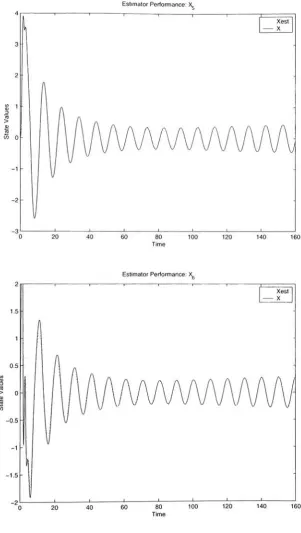
other subsystems are

3

Controller

Design

and

Stability

Analysis

The

problem presented

in

this

paper

is

to

design

a

distributed

controller

in

the

form

of

(2.31)

that

will

force

the

system states of

(2.17)

to

track

the

states of

the

desired

reference model

(2.10).

In

addition,

an adaptive state estimator

is designed for

each

subsystem which enables a reduction

in

the

required amount of

inter-node

commu

nications.

The

approach presented

here is

to

design

the

controller and estimator

parameters

using

an adaptive method

based

on

Lyapunov

stability

analysis.

Thus,

the

adaptive updates

for

the

controller and estimator parameters will

be

selected so

as

to

ensure

stability

of

the

tracking

errors

e*

and state estimation errors Xj.

In

order

to apply the

Lyapunov

stability

analysis

techniques

to the

proposed

distributed

control

scheme,

a separate

Lyapunov function (VA

will

be

identified

for

each subsystem.

The

stability

of

the

overall system can

then

be

concluded

using the

following

Lyapunov function:

M

v

=

Y^

(3-41)

2=₁

Upon

close

inspection

of

(2.31),

it is

obvious

that there

are

two

cases which require

separate consideration

in

the stability

analysis: x

G

Qi

and x

G

Q2

as

defined

in

(2.30).

Each

of

these

cases will

be

considered

separately

below.

3.1

No Adaptation

The first

case

to

be

considered

is

when

the

system state vector

is

within region

Qi

as

defined

by,

xEQi:eJei<ElQ,\/t

(3.42)

In

this case, there

is

no communicationof

the

local

statevectors

between

subsystems.

This

means

that

at each

node, the

estimator outputs

Xj

will

be

used

to

calculate

the

controller output

u{

at each

sampling instant

(see

equation

2.31).

Adaptation

of

the

estimator and

the

controller parameters

does

not occur

for

x

G

fy.

During

this

tracking

error.

It

is

assumed

that the

bounds

El0

are set such

that

the

performance

of

the

system

is

considered acceptable as

long

as x

G

^i.

In

this case,

because

the

system states are upper

bounded

by

the

given

threshold

values

ElQ,

the

system

is

bounded-input

bounded-output

(BIBO)

stable

by

assumption.

3.2

During

Adaptation

The

second case

to

be

considered

is

when

the

system state vector

is

within region

fl2

as

defined

by,

x

G

02

:

3z

|

ef

e%

>

El0

(3.43)

In

this case, the

estimator and

the

controller parameters will

be

adapted

in

an effort

to

drive

the

system states

towards those

of

the

reference model

(and

thus to

drive

the

system state vector

back into

region

fij).

In

addition,

communication

between

subsystems will

be occurring

such

that the

entire system state vector x will

be known

to

each subsystem.

This

means

that the

ith

subsystem will

have

access

to the

actual

state vectors

Xj

rather

than

just

the

estimates Xj.

This information

can

then

be

used

to

calculate

the

local

controller output

Ui

as well as

the

adaptive updates

to

local

controller and state estimator parameters.

For

these conditions,

Lyapunov

stability

theory

will

be

used

to

determine

the

appropriate controller updates

that

guarantee

stability

of

the

overall system.

In

order

to simplify the

development,

the stability

of

the

adaptive controller and

the

adaptive

state estimators are considered

separately

below.

3.2.1

Adaptive Controller

Following

the

development in

[6],

consider

the

following

Lyapunov function

can

didate for

the

ith

subsystem:

M

where,

ki

=

ki-K*

(3.45)

i>ij

=

i>ij

-ipij

(3-46)

and

Bi

is

a positive-definite matrix

that

is

the

solution

to the

following

Lyapunov

equation:

ATmiBi

+

BtAmi

=

-Qt

(3.47)

It is

clear

by

inspection

that the

function

in

(3.44)

is

positive

definite.

Taking

the

time

derivative

of

this

equation

along

the

system

trajectory

then

gives

the

following:

.

x M ._ .

x

Vl

=

eTBlel + elBlel +

k7kl

+

kikl+

Y

$!&,

+

A^j]

(3-48)

j=i,j&

Referring

to

(2.29),

the time-derivative

of

the

state

tracking

error can

be

written as

follows:

6i

Xi

xmi

^o.^ty

j

Substitution

of

(2.12)

and

(2.20)

into

this

equation

then

gives:

M

<=;

=

AiXi

+

Bi[Kjxi

-Y

V?xj

+

ri\ +

AmiXi

~

Biri

(3-50)

Now,

using

(2.21)

the

equation above can

be

rearranged

to

give:

e, =

BiKf

Xi +

Amie%

+

Bt

Y

Wjx3

(3-51)

The last four

terms

in

(3.48)

involve

the

time-derivatives

of

the

controller parameter

definitions

of

the

errors

themselves

as

follows:

Ki

= Kt-K*

(3.52)

Ki

=

Ki

(3.53)

Similarly,

for

the

error

in

the

estimates of

the

interaction

terms:

ipij

=

i>ij

~

ipij

iii

=

-A3

(3-54)

Following

the

development

in

[6],

the

proposed adaptive updates are as

follows:

Kj

=

-ejBiB.xf

(3.55)

ipzj

=

eTPiBixj

(3.56)

Substitution

of

(3.55