Deep depth-based representations of graphs through deep learning networks

This is a repository copy of

Deep depth-based representations of graphs through deep

learning networks

.

White Rose Research Online URL for this paper:

http://eprints.whiterose.ac.uk/130212/

Version: Accepted Version

Article:

Bai, Lu, Cui, Lixin, Bai, Xiao et al. (1 more author) (2018) Deep depth-based

representations of graphs through deep learning networks. Neurocomputing. ISSN

0925-2312

https://doi.org/10.1016/j.neucom.2018.03.087

[email protected]

Reuse

This article is distributed under the terms of the Creative Commons Attribution-NonCommercial-NoDerivs

(CC BY-NC-ND) licence. This licence only allows you to download this work and share it with others as long

as you credit the authors, but you can’t change the article in any way or use it commercially. More

information and the full terms of the licence here: https://creativecommons.org/licenses/

Takedown

If you consider content in White Rose Research Online to be in breach of UK law, please notify us by

Deep Depth-based Representations of Graphs through Deep

Learning Networks

Lu Bai1∗

, Lixin Cui1∗

, Xiao Bai2, Edwin R. Hancock3 1_{Central University of Finance and Economics, Beijing, China.}

2_{Beihang University, Beijing, China.} 3_{University of York, York, UK.}

Abstract

Graph-based representations are powerful tools in structural pattern recognition and

machine learning. In this paper, we propose a framework of computing the deep

depth-based representations for graph structures. Our work links the ideas of graph

complexity measures and deep learning networks. Specifically, for a set of

graph-s, we commence by computing depth-based representations rooted at each vertex as

vertex points. In order to identify an informative depth-based representation subset,

we employ the well-knownk-means method to identifyMdominant centroids of the

depth-based representation vectors as prototype representations. To overcome the

bur-densome computation of using depth-based representations for all graphs, we propose

to use the prototype representations to train a deep autoencoder network, that is

opti-mized using Stochastic Gradient Descent together with the Deep Belief Network for

pretraining. By inputting the depth-based representations of vertices over all graphs to

the trained deep network, we compute the deep representation for each vertex. The

re-sulting deep depth-based representation of a graph is computed by averaging the deep

representations of its complete set of vertices. We theoretically demonstrate that the

deep depth-based representations of graphs not only reflect both the local and global

characteristics of graphs through the depth-based representations, but also capture the

main structural relationship and information content over all graphs under

investiga-tions. Experimental evaluations demonstrate the effectiveness of the proposed method.

∗_{These authors contribute equally to this work and are co-first authors} *Manuscript

Keywords: Depth-based Representations, Deep Representations, Deep Autoencoder

Networks, Prototype Representations

1. Introduction

Analyzing data using graph-based representations has attracted an increasing

in-terest in machine learning and pattern recognition, due to the representational

pow-er of graph structures. Typical applications include a) analyzing bioinformatics and

chemoinformatics data [1] (e.g., classifying graph-based representations of proteins or

5

chemical compounds into different species), b) recognizing graph-based object

descrip-tions from images [2], c) visualizing social networks [3] (e.g., Twitter and Facebook

friendship networks, DBLP citation networks), etc. One challenge arising in

analyz-ing graph-based representations of data is how to convert the discrete graph structures

into numeric features, since this allows standard pattern recognition techniques to be

10

directly applied to graphs.

The aim of this paper is to propose a new framework of computing deep

depth-based representation of a graph through the use of deep learning networks [4]. Our

ap-proach is to identify a family of dominant depth-based representations [5] as prototype

representations, and then train a deep network that can better preserve the non-linear

15

graph structure information. The resulting deep depth-based representations of graphs

are computed through the trained deep networks.

1.1. Literature Review

Although graph-based representations are powerful tools for structural pattern

recog-nition, the main drawback associated with graph structures is the lack of a

correspon-20

dence order or labels for the vertices, i.e., we do not explicitly know how to align

different graph adjacency matrices. Compared to vector-based pattern recognition, this

in turn limits the set of standard machine learning algorithms that can be directly

ap-plied to problems of graph classification or clustering [6]. One way to overcome this

problem is to convert the graph structures into a numeric characteristics [7].

25

Generally speaking, most existing methods can be categorized into two classes,

graph kernel to characterize the similarity of different graph structures in a high

di-mensional Hilbert space. Proponents of the first class of methods tend to represent

graphs as permutation invariant features in a vector space, where standard machine

30

learning techniques designed for vector-based data can be directly employed. For

in-stance, Wilson et al. [8] have computed graph invariant from algebraic graph theory.

They use the spectral decomposition of a Hermitian property matrix as the complex

analogue of the Laplacian, and construct symmetric polynomials associated with the

eigenvectors. Bunke et al. [7] have embedded graphs into vectors by employing both

35

vertex and edge attributed statistics. Ren et al. [9] have computed vectorial graph

fea-tures via the Ihara zeta function. They first transform each graph into a directed line

graph and then identify the cycles residing on the line graph. The resulting graph

fea-tures are computed by counting the number of cycles having different lengths. Kondor

and Borgwardt [10] have computed invariant graph skew spectrum features, by

map-40

ping each graph adjacency matrix into a symmetric group function and computing the

associated bispectral invariants. Bai and Hancock [11] have developed a framework to

compute depth-based representations of graphs. Specifically, they first decompose each

graph into a family of expansion subgraphs with increasing size, and then measure the

entropy-based information content of these substructures. Unfortunately, these

state-45

of-the-art methods tend to approximate graph structures in a low dimensional vector

space, and thus discard correlation information. By contrast, the proponents of graph

kernels can characterize graphs in a high dimensional Hilbert space and thus better

preserve the structural correlations of graphs [12].

One of the most generic frameworks of defining graph kernels is the concept of

50

R-convolution proposed by Haussler [13]. The main idea underpinning R-convolution

graph kernels is that of decomposing graphs into substructures of limited sizes and

then comparing pairs of specific substructures, such as walks, paths, subtrees and

sub-graphs. Under this scenario, Kashima et al. [14] have defined a marginalized kernel by

comparing pairs of random walks associated with vertex and edge labels. Costa and

55

Grave [15] have proposed a pairwise neighborhood subgraph distance kernel, by

count-ing pairs of isomorphic pairwise neighborhood subgraphs. Bach [16] has proposed a

graphical model on the subtrees. Wang and Sahbi [17] have defined a graph kernel for

action recognition, by describing actions as directed acyclic graphs (DAGs) and

count-60

ing the number of isomorphic walk pairs. Harchaoui and Bath [18] have proposed

a segmentation graph kernel for images by counting the inexact isomorphic subtree

patterns between image segmentation graphs. Bai et al. [19] have defined an aligned

subtree kernel by counting pairs of inexact isomorphic subtrees rooted at aligned

ver-tices. Alternative state-of-the-art graph kernels based on R-convolution include a) the

65

subtree-based hypergraph kernel [20], b) the subgraph matching kernel [1], c) the

opti-mal assignment kernel [21], d) the aligned Jensen-Shannon subgraph kernel [22], and

e) the fast depth-based subgraph kernel [23].

Unfortunately, as we have stated, the R-convolution graph kernels usually employ

substructures of limited sizes. As a result, most of the aforementioned kernels only

70

reflect local graph characteristics, i.e., these kernels cannot capture characteristics of

graph structures at the global level. To address this problem, Bai et al. [2, 24] have

developed a family of graph kernels based on information theoretic measures, namely

the classical and quantum Jensen-Shannon divergence. Specifically, they use either the

classical or the quantum random walk associated with the divergence to measure the

75

similarity between graphs at a global level based on entropies. Johansson et al. [25]

have developed a global graph kernel based on geometric embeddings. Specifically,

they use the Lov´asz number as well as its associated orthonormal representation to

capture the characteristics at a global level.

One common weakness arising in most of the aforementioned state-of-the-art

meth-80

ods, either graph embedding methods or graph kernels, is that of ignoring information

from multiple graphs. This is because the graph embedding method usually captures

characteristics for each single graph structure. On the other hand, the graph kernel

only reflects graph characteristics for each pair of graphs. As a summary, developing

effective method to preserve the structural information residing in graphs still remains

85

1.2. Contribution

To overcome the shortcoming of both existing graph embedding methods and graph

kernels, in this paper, we aim to present a novel framework for computing deep

depth-based representations for graph structures. Our work links the ideas from graph

com-90

plexity and deep learning networks [4]. In particular, for a set of graphs under analysis,

we commence by computing the depth-based representations rooted at each vertex [23].

This is done by decomposing a graph structure into a family of expansion subgraphs

of increasing sizes rooted at a vertex, and then measuring the entropy-based

complexi-ties of the subgraphs and use this to construct a complexity trace, i.e., the depth-based

95

representation of the root vertex. Since the complexity trace encapsulates entropic

information flow from the root vertex to the global graph structure, the depth-based

representation can simultaneously capture both local and global graph characteristics.

With the depth-based representations of vertices over all graphs to hand, we

em-ploy the well-knownk-means method [26] to identifyk dominant centroids of these

100

depth-based representation vectors as prototype representations. Since the prototype

representations are identified by minimizing the sum of square distances between all

depth-based representations and the centroid points (i.e., the prototype representations)

of their clusters, the prototype representations can reflect representative characteristics

of all depth-based representations encountered. As a result, the prototype

representa-105

tions can encapsulate dominant characteristics over all used graphs.

In order to reflect the high dimensional structural information of graphs well, we

propose to further capture the manifolds of these prototype representations using deep

learning networks [4]. This is motivated by the recent success of deep learning [3, 27],

that has been proven a powerful tool of learning complex relationships of data [28].

110

Specifically, with the prototype representations as input data, we train a deep neural

network (i.e., the deep autoencoder network [3]) that is optimized using Stochastic

Gra-dient Descent together with the Deep Belief Network [29] for pretraining. Note that,

training the deep network associated with the smaller set of prototype

representation-s can representation-significantly reduce the burdenrepresentation-some computation arepresentation-srepresentation-sociated with depth-barepresentation-sed

115

representations of all graphs. Since the deep autoencoder network can minimize the

the dominant structural information over the vertices of all graphs, the deep network

can capture the salient information for these graphs in a highly non-liner latent space.

By inputting the depth-based representations of vertices over all graphs to the trained

120

deep network, we compute the deep representation for each vertex. The resulting deep

depth-based representation of a graph is computed by averaging the deep

representa-tions of all its vertices. We theoretically demonstrate that the deep depth-based

repre-sentations of graphs not only reflect both the local and global characteristics of graphs

through the depth-based representations, but also capture the main relationships and

125

information over all graphs under investigations. Experimental evaluation demonstrate

the effectiveness of the proposed method.

1.3. Paper Outline

The remainder of this paper is organized as follows. Section 2 reviews the

prelimi-nary concepts that will be used in this work. Section 3 details the proposed framework

130

for computing deep depth-based representations of graphs. Section 4 provides the

ex-perimental evaluation of the new method. Section 5 concludes this work.

2. Preliminary Concepts

In this section, we review some preliminary concepts that will be used in this work.

We commence by reviewing the concept of depth-based representation from

entropy-135

based complexity measures. Finally, we show how to identify the k dominant centroids

of the depth-based representation vectors as prototype representations based on the

well-knownk-means clustering method.

2.1. Depth-Based Representations

In this subsection, we review how to compute the depth-based representation

root-140

ed at each vertex of a graph [23]. The depth-based representation is a powerful tool

for characterizing the topological structure in terms of the intrinsic complexity. One

way of computing the representation is to gauge the information content flow through

a family of K-layer subgraphs of a graph (e.g., subgraphs around a vertex having

min-imal path length K) of increasing size and to use the flow as a structural signature. By

measuring the entropy measure of each expansion subgraph, Bai et al. [23] have shown

how to use this this to characterize each graph as a depth-based complexity trace

repre-sentation that gauges how the entropy-based complexities of the expansion subgraphs

vary as a function of depth.

Specifically, assume a sample graph is denoted asG(V, E), whereV andEare the

vertex and edge sets respectively. We first compute the shortest path matrix ofG(V, E)

asSGbased on the well-known Dijkstra’s algorithm. Note thatSGfollows the same

vertex permutation with the adjacency matrix ofGand each elementSG(v, u)indicates

the shortest path length between verticesuandv. Assume the neighbourhood vertex

set ofv∈V is denoted asNK

v and satisfies

N_vK ={u∈V |SG(v, u)≤K}. (1)

For each vertexv∈VofG(V, E), a family ofK-layer expansion subgraphsGK

v(VK;EK)

rooted atvis defined as

⎧

⎨

⎩ VK

v ={u∈NvK};

EK

v ={(u, v)⊂NvK×NvK|(u, v)∈E}.

(2)

Note that theK-layer expansion subgraphGK

v is the global structure ofG(V, E)ifK

150

is equal or larger than the length of the greatest shortest path starting from vertexvto

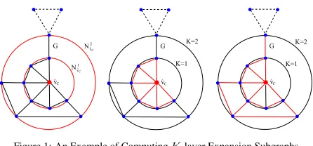
the remaining vertices ofG(V, E). Fig.1 gives an example to explain how to compute

aK-layer expansion subgraph rooted at a sample vertexˆvC∈V. The left-most figure

shows the determination ofK-layer expansion subgraphs for a graphG(V, E)which

hold|N_ˆv1_C|= 6and|N_vˆ2_C|= 10vertices. While the middle and the right-most figure

155

show the corresponding1-layer and2-layer subgraphs regarding the vertexvˆC, and are

depicted by red-colored edges. In this example, the vertices of differentK-layer

sub-graphs regarding the vertexˆvCare calculated by Eq.(1), and pairwise vertices possess

the same connection information in the original graphG(V, E).

Definition (Depth-based representations of vertices): For the graphG(V, E), let

the family ofK-layer expansion subgraphs rooted at each vertexv ∈ V be denoted

as{G1

depth-Figure 1: An Example of ComputingK-layer Expansion Subgraphs.

based representationDBL

v of vertexvis defined as

DBL

v ={HS(Gv1),· · ·, HS(GKv),· · ·, HS(GvL)}, (3) whereK≤LandHS(GvK)is the Shannon entropy ofGvKcomputed using the steady

160

state random walk [2]. ✷

We observe a number of interesting properties for the depth-based representation.

First, it is computed by measuring the entropy-based complexity on the gradually

ex-panding subgraphs rooted at a vertex, and thus encapsulates rich intrinsic depth

com-plexity information rooted at the vertex. Second, since the computational comcom-plexity

of the required Shannon entropy associated with the steady state random walk is only

quadratic in the number of vertices [2], the depth-based representation can be

efficient-ly computed [23]. Furthermore, based on Eq.(2), we observe that the famiefficient-ly ofK-layer

expansion subgraphs rooted at a vertexvsatisfy

v∈Gv1· · ·⊆GvK ⊆· · ·⊆GLv ⊆G.

This observation indicates that these expansion subgraphs form a nested sequence, i.e.,

the sequence of subgraphs gradually expand from the local vertexvto the structure

of the global graph. As a result, the depth-based representation can simultaneously

capture the local and global graph structure information.

165

2.2. Identifying Prototype Representations

In this subsection, we identify the centroids over all depth-based representation

vec-tors. In particular, assume a set ofNgraphs is denoted asG_{={G1,· · ·, Gi,· · ·, GN}.} Based on Eq.(3), for each graphGi we commence by computing theL-dimensional

nvertices over all graphs inG_{, and theL-dimensional depth-based representations of}

these vertices areDBL_{= (DB}L₁,DB2L, . . . ,DBLn). We use thek-means method [26] to identifyM centroids over all depth-based representations inDBL_{, i.e., we divide}

these representations intoM clusters and compute the mean vector for each cluster.

Specifically, givenMclustersΩ = (cL

1, cL2, . . . , cLM)whereLcorresponds to the pa-rameter of theseL-dimensional depth-based representations, thek-means method aims

to minimize the following objective function

arg min

Ω

N

$

i=1

$

DBL j∈cLi

∥DBL j −µ

L

i∥2, (4)

whereµLi is the mean of the depth-based representation vectors belonging to clustercLi.

Since Eq.(4) minimizes the sum of the square Euclidean distances between the vertex

pointsDBL

j and their centroid point of clustercLi, theMcentroid points{µL1,· · ·, µLM} can reflect main characteristics of all L-dimensional depth-based representations in

170

DBL_{. In other words, these centroid can be seen as a family ofL-dimensional}

pro-totype representations that encapsulate representative characteristics over all graphs in

G_.

3. Deep Depth-based Representations of Graphs

In this section, we introduce a framework of computing the deep depth-based

rep-175

resentations of graphs, by linking the ideas of depth-based complexity measures and

the powerful deep learning networks. We commence by reviewing the concept of deep

autoencoder network [29]. Finally, we show how to compute the deep depth-based

representation through the deep network.

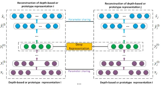
3.1. Deep Autoencoder Networks 180

In this subsection, we briefly review the concept of deep autoencoder, that is a

deep learning network [29]. This network is one kind of unsupervised model and is

composed of a encoder network and a decoder network. The encoder network consists

of multiple non-linear functions that map the input data to a representation space, i.e.,

the encoder network transforms the original data into the deep representations [3]. On

Figure 2: The Architecture of the Deep Autorencode Network.

Table 1: Terms and Notations

Symbol Definition

n number of vertexes

K number of layers

S={s1, ..., sn} the adjency matrix for the network

X={xi}ni=1,Xˆ={ˆxi}ni=1 the input data and reconstructed data

Yk

={yk i}

n

i=1 the k-th layer hidden representation

Wk,Wˆk the k-th layer weight matrix

bk_,ˆbk _{the k-th layer biases}

θ(k)_={Wk_,Wˆk_{, b}k_,ˆbk

} the overall parameters

the other hand, the decoder network consists of multiple non-linear functions mapping

the deep representations in the representation space to the reconstruction space, i.e., the

decoder network reconstructs the original data based on the deep representations. It has

been proven that the deep representation between the encoder and decoder networks

smoothly captures the data manifold embedded in a highly non-liner space. As a result,

190

the deep representation enhances the linear separability of the original data [29], and

provides an elegant way of analyzing the original data.

The architecture of the deep autoencouder network used in this work is shown in

is the input, then the hidden representations for each layer are computed as

yk i =

⎧

⎨

⎩

σ_(W(1)_x

i+b(1)) ifk= 1;

σ_(W(k)_yk−1

i +b(k)) ifk= 2, ..., K.

(5)

AfterKsteps, we obtainy(_iK)through the encoder network, i.e., we transformxiinto

y_i(K)(the deep representation ofxi). Then, after anotherKsteps, we can obtain the outputxˆiby reversing the calculation process of encoder through the decoder network,

i.e., we reconstruct the inputxiasxˆithroughyi(K). The objective of the deep autocoder network is to minimize the reconstruction error of outputxˆiand inputxi, and the loss

function is defined as

L=

n

$

i=1

∥xˆi−xi∥22 (6)

To optimize the deep autocoder network, we first use the Deep Belief Network [29]

to pretrain its parameters to avoid trapping in local optimum in the parameter space.

Then, the deep network is optimized by means of the Stochastic Gradient Descent

195

method, where the gradients can be conveniently obtained by applying the chain rule

to backpropagate error derivatives first through the decoder network and then through

the encoder network, i.e., back-propagate∂∂θLto updateθ k_.

As [3] stated, although the reconstruction process does not explicitly preserve the

original inputxi, minimizing the reconstruction error can smoothly capture the

mani-200

folds of original data and thus capture the main characteristics of the data.

3.2. The Deep Representation through Deep Networks

In this subsection, we propose a new deep depth-based representation that

repre-sents a graph as embedding vector. LetG_={G1,· · ·, Gi,· · ·, GN}be a set of graph-s. For each graphGi(Vi, Ei) ∈ G, we commence by computing theL-dimensional

depth-based representation of each vertexv∈Vibased on Eq.(3) as

DBL

i;v={HS(Gi1;v),· · ·, HS(GiK;v),· · ·, HS(GiL;v)},

where the subscriptsi,vandLcorrespond to the graphGi∈G, the vertexv∈Viand

definition in Section 2.2, we identify a family ofL-dimensional prototype

representa-tions. Specifically, with theL-dimensional depth-based representations of all graphs in

G_{to hand, we perform thek-means method to identifyMcentroids, i.e., we divide the}

depth-based representations intoMclusters and compute the means{µL

1,· · ·, µLM}of these clusters as theL-dimensional prototype representations. We further use the

pro-totype representations{µL

1,· · ·, µLM}as input data to train a deep autoencoder network proposed in Section 3.1. Training the deep network using the smaller set of prototype

representations not only avoids the burdensome computation of using depth-based

rep-resentations of all graphs inG_{, but also preserves the dominant information of these}

graphs for the training process. With the trained deep autoencoder network to hand,

for each graphGi(Vi, Ei)∈G, we use itsL-dimensional depth-based representations

DBs_G

i={DB

L

i;1,· · ·,DBLi;v,· · ·,DB L

i;|Vi|}rooted at all vertices inVias input, here the subscripts1to|Vi|ofDBsGicorrespond to the1-th toVi-th vertex inVi. Based

on Eq.(5) we obtain a set of|V|deep representation vectors of all vertices inVias

DRs_G i={y

(K)

1 ,· · ·, y(vK), . . . , y

(K)

|Vi|}, (7)

wherey(vK)is the deep representation ofDBLi;v, i.e.,y

(K)

v is the deep representation of

vertexv∈ViforGi. Then, the deep representation ofGiis

DRGi=

$

v∈_|Vi|

y(vK), (8)

i.e.,DRGiis the mean vector of the deep representation vectors inDRsGi. The

re-sulting deep depth-based representationDDBGi of each graphGi ∈ Gis computed

by performing the Principle Component Analysis (PCA) [30] on the graph deep

rep-205

resentation matrixDRG = (DRG1| · · · |DRGi| · · · |DRGN)to embed the each deep

representationDRGiofGiin a principle space. Since the deep representationDRGi

of each graphGican effectively capture the manifold of all graphs in the deep space,

the deep depth-based representationDDBGi enhances the linear separability of the

graphs. The algorithm of computing the deep depth-based representation is shown in

210

Algorithm 1Vertex labels strengthening procedure Input:A set of graphsG_={G1,· · ·, Gi,· · ·, GN}.

Output: The deep depth-based representationDDBG_iof each graphGi, and parametersθof

the Deep Autoencoder Network (DAN).

1: Initalization

• For each graphGi(Vi, Ei)∈G, compute theL-dimensional depth-based representations

DBL

i;vfor each vertexv∈Vibased on Eq(3).

• Use thek-means method to divide the depth-based representation vectors of all graphs in

GintoMclusters and compute these cluster means{µL1,· · ·, µ

L

M}as theL-dimensional

prototype representations.

2: Train the DAN with Parameters in Table.1.

• Input the prototype representations as the input dataX, and pretrain DAN through Deep

Belief Network to initialize the parametersθ_={θ(1)_{,· · ·,}θ(K)_{}for DAN.}

• Repeat

• Based onXandθ, computeXˆusing Eq.(5).

• Compute the least square error betweenXˆandXasL=!n

i=1∥Xˆ−X∥ 2 2.

• Using the Stochastic Gradient Descent to updateθ, i.e., back-propagate∂L

∂θ to updateθ.

• Untilconverge

3: Compute Deep Depth-based Representations.

• Based on Eq.(7) and (8), compute the deep representation DRG_i for each graph

Gi through the trained DAN, perform PCA on the deep representation matrix

DRG = (DRG₁| · · · |DRGi| · · · |DRG_N)to compute the deep depth-based

3.3. Discussions and Related Works

The deep depth-based representationDDBGiof a graphGi∈Gproposed in

Sec-tion 3.2 has a number of advantages.

First, unlike most state-of-the-art graph kernels mentioned in Section 1.1, the

pro-215

posed deep depth-based representationDDBGi can simultaneously capture the local

and global graph characteristics. This is because the associated depth-based

repre-sentation for our framework is computed from the entropy measures on the family of

expansion subgraphs, that gradually lead a local vertex to the global graph structure. By

contrast, the mentioned R-convolution graph kernels [1, 14, 15, 16, 17, 18, 19, 20, 23]

220

are computed by comparing pairs of subgraphs of limited sizes (e.g., paths, cycles,

walks, subgraphs and subtrees), and thus only reflect local topological information

of graphs. On the other hand, the graph kernels based on the classical and quantum

Jensen-Shannon divergence [2, 24], as well as the Lov´asz graph kernel [25] are

com-puted based on global graph characteristics (e.g., Shannon or von Neumann entropies,

225

and Lov´asz number associated orthonormal representation). These kernels can reflect

global graph characteristics, but tend to ignore local graph information. As a summary,

most existing graph kernels cannot reflect complete information of graph structures.

Second, unlike most state-of-the-art graph embedding methods mentioned in

Sec-tion 1.1, the proposed deep depth-based representaSec-tionDDBGi can effectively

cap-230

ture the manifold of the graphs in a highly non-liner latent space, and thus reflect rich

characteristics of graph structures. This is because the deep depth-based

represen-tationDDBGiis computed through the powerful deep autoencoder network, that can

smoothly capture the data manifold in a highly non-linear space. By contrast, the graph

embedding methods [6, 7, 8, 7, 9, 10, 11] tend to embed graphs from high dimensional

235

structure space in a low dimensional vectorial space, and thus lead to information loss.

Third, unlike the state-of-the-art graph kernels and graph embedding methods, the

proposed deep depth-based representationDDBGi can reflect comprehensive

charac-teristics of all graph under investigations. This is because the required deep

autoen-couder network is trained by using the prototype representations. These

representa-240

tions are identified by employing thek-means clustering method on the depth-based

S-ince the prototype representations can represent the main characteristics of all graphs,

the deep autoencoder network trained from these representations can simultaneously

capture the main information of all graphs. As a result, the deep depth-based

repre-245

sentationDDBGicomputed through the deep autoencouder network can encapsulate

all graph characteristics. By contrast, most existing graph kernels [1, 14, 15, 16, 17,

18, 19, 20, 23] compute the kernel value based on pairs of graphs. On the other hand,

the graph embedding methods [6, 7, 8, 7, 9, 10, 11] compute the graph feature vector

based on each individual graph.

250

Finally, note that, the depth-based complexity traces [11] and the fast depth-based

subgraph kernel [23] are also based on the depth-based representations. Thus, similar

to the proposed deep depth-based representation, these two existing methods can

si-multaneously capture the local and global graph characteristics too. However, as one

kind of graph embedding method, the depth-based complexity trace can only represent

255

graphs in low dimensional vectorial space, and leads to information loss. By contrast,

the proposed method can capture richer graph characteristics through the powerful deep

autoencoder network. Furthermore, both the depth-based complexity trace and the fast

depth-based graph kernel suffer from the drawback of ignoring comprehensive

infor-mation over all graphs under investigations, because these methods only capture graph

260

information for each individual graph or pairs of graphs.

The above observations reveal the theoretical effectiveness of the proposed deep

depth-based representation. The proposed method provides an effective way of

analyz-ing graph structures for classification or clusteranalyz-ing problems.

3.4. Computational Analysis 265

The computational complexity of the proposed deep depth-based representation is

governed by the following computational steps. Consider a set ofNgraphs each having

Svertices andT edges, and the greatest lengthLof the shortest paths over all these

graphs. Computing the depth-based representations of vertices for each graph relies on

the calculation of the shortest path matrix, and thus computing the representations of all

270

graphs requires time complexityO(Nlog(S)T). The identification of theMprototype

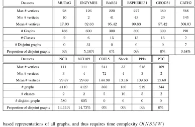
depth-Table 2: Information of the Graph-based Datasets

Datasets MUTAG ENZYMES BAR31 BSPHERE31 GEOD31 CATH2

Max # vertices 28 126 220 227 380 568

Min # vertices 10 2 41 43 29 143

Mean # vertices 17.93 32.63 95.42 99.83 57.42 308.03

# Graphs 188 600 300 300 300 190

# Classes 2 6 15 15 15 2

# Disjoint graphs 0 31 0 0 0 7

Proportion of disjoint graphs 0% 5.16% 0% 0% 0% 3.68%

Datasets NCI1 NCI109 COIL5 Shock PPIs PTC

Max # vertices 111 111 241 33 218 109

Min # vertices 3 4 72 4 3 2

Mean # vertices 29.87 29.68 144.90 13.16 109.63 25.60

# graphs 4110 4127 360 150 219 344

# classes 2 2 5 10 5 2

# disjoint graphs 580 605 0 0 0 0

Proportion of disjoint graphs 14.11% 14.73% 0% 0% 0% 0%

based representations of all graphs, and thus requires time complexityO(N SM W)

where W is the iteration number. Training the deep autoencoder network requires

time complexityO(LDCI), whereLcorresponds to the dimension of input data,D

275

is the degree of the deep network,C is the dimension of the hidden layers andI is

the iteration. As a result, computing the deep depth-based representations of all graphs

requires time complexityO(Nlog(S)T+N SM W+LDCI).

4. Experimental Results

In this section, we empirically evaluate the performance of the proposed deep

280

depth-based representations of graphs. We commence by testing the proposed method

on the graph classification problem using standard graph datasets that are abstracted

from bioinformatics and computer vision databases. Furthermore, we also compare the

proposed method with several state-of-the-art methods, e.g., graph kernels and graph

embedding methods.

4.1. Graph Datasets

We demonstrate the classification performance of the proposed method on twelve

standard graph-based datasets abstracted from both bioinformatics and computer

vi-sion datasets. These datasets include: MUTAG, ENZYMES, BAR31, BSPHERE31,

GEOD31, CATH2, NCI1, NCI109, COIL5, Shock, PPIs, and PTC(MR). More details

290

concerning the datasets are shown in Table.2.

MUTAG: The MUTAG dataset consists of graphs representing 188 chemical

com-pounds, and here the goal is to predict whether each compound possesses

mutagenic-ity [31]. The maximum, minimum and average number of vertices are 28, 10 and

17.93 respectively. As the vertices and edges of each compound are labeled with a real

295

number, we transform these graphs into unweighted graphs.

ENZYMES:The ENZYMES dataset consists of graphs representing protein tertiary

structures, and contains 600 enzymes from the BRENDA enzyme database [32]. In

this case, the task is to correctly assign each enzyme to one of the 6 EC top-level

classes. The maximum, minimum and average number of vertices are 126, 2 and 32.63

300

respectively.

BAR31, BSPHERE31 and GEOD31: The SHREC 3D Shape database consists of

15classes and 20 individuals per class, that is 300 shapes [33]. This is a standard

benchmark in 3D shape recognition. From the SHREC 3D Shape database, we

estab-lish three graph datasets named BAR31, BSPHERE31 and GEOD31 datasets through

305

three mapping functions. These functions are a) ERG barycenter: distance from the

center of mass/barycenter, b) ERG bsphere: distance from the center of the sphere that

circumscribes the object, and c) ERG integral geodesic: the average of the geodesic

distances to all other points. Details of the three mapping function can be found in

[33]. The number of maximum, minimum and average vertices for the three datasets

310

are a) 220, 41 and 95.42 (for BAR31), b) 227, 43 and 99.83 (for BSPHERE31), and c)

380, 29 and 57.42 (for GEOD31), respectively.

CATH2:The CATH2 dataset has proteins in the same class (i.e., Mixed Alpha-Beta),

architecture (i.e., Alpha-Beta Barrel), and topology (i.e., TIM Barrel), but in different

homology classes (i.e., Aldolase vs. Glycosidases). The CATH2 dataset is harder to

315

protein graphs are10times larger in size than chemical compounds, with200−300

vertices. There is190testing graphs in the CATH2 dataset.

NCI1 and NCI109: The NCI1 and NCI109 datasets consist of graphs representing

two balanced subsets of datasets of chemical compounds screened for activity against

320

non-small cell lung cancer and ovarian cancer cell lines respectively [34]. There are

4110 and 4127 graphs in NCI1 and NCI109 respectively.

COIL5: We establish a COIL5 dataset from the COIL database. The COIL image

database consists of images of 100 3D objects. We use the images for the first five

objects. For each object we employ 72 images captured from different viewpoints. For

325

each image we first extract corner points using the Harris detector, and then establish

Delaunay graphs based on the corner points as vertices. As a result, in the dataset there

are 5 classes of graphs, and each class has 72 testing graphs. The number of maximum,

minimum and average vertices for the dataset are 241, 72 and 144.90 respectively.

Shock:The Shock dataset consists of graphs from the Shock 2D shape database. Each

330

graph is a skeletal-based representation of the differential structure of the boundary of a

2D shape. There are 150 graphs divided into 10 classes. Each class contains 15 graphs.

PPIs: The PPIs dataset consists of protein-protein interaction networks (PPIs). The

graphs describe the interaction relationships between histidine kinase in different species

of bacteria. Histidine kinase is a key protein in the development of signal transduction.

335

If two proteins have direct (physical) or indirect (functional) association, they are

con-nected by an edge. There are 219 PPIs in this dataset and they are collected from 5

different kinds of bacteria (i.e., a)Aquifex4 andthermotoga4 PPIs fromAquifex

aeli-cusandThermotoga maritima, b)Gram-Positive52 PPIs fromStaphylococcus aureus,

c)Cyanobacteria73 PPIs fromAnabaena variabilis, d) Proteobacteria40 PPIs from

340

Acidovorax avenae, and e)Acidobacteria46 PPIs). Note that, unlike the experiment

in [24] that only uses theProteobacteria40 and theAcidobacteria46 PPIs as the

test-ing graphs, we use all the PPIs as the testtest-ing graphs in this paper. As a result, the

experimental results for some kernels are different on the PPIs dataset.

PTC:The PTC (The Predictive Toxicology Challenge) dataset records the

carcino-345

genicity of several hundred chemical compounds for male rats (MR), female rats (FR),

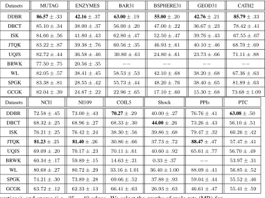
Table 3: Classification Accuracy (In%±Standard Error) Comparisons

Datasets MUTAG ENZYMES BAR31 BSPHERE31 GEOD31 CATH2

DDBR 86.57±.33 42.16±.37 63.00±.19 55.00±.20 42.76±.21 85.79±.33

DBCT 85.10±.34 38.00±.37 56.00±.20 47.00±.22 36.67±.23 78.42±.41

ISK 84.66±.56 41.80±.43 62.80±.47 52.50±.47 39.76±.43 67.55±.67

JTQK 83.22±.87 39.38±.76 60.56±.35 46.93±.61 40.10±.46 68.70±.69

UQJS 82.72±.44 36.58±.46 30.80±.61 24.80±.61 23.73±.66 71.11±.88

BRWK 77.50±.75 20.56±.35 _{−− −− −− −−}

WL 82.05±.57 38.41±.45 58.53±.53 42.10±.68 38.20±.68 67.36±.63

SPGK 83.38±.81 28.55±.42 55.73±.44 48.20±.76 38.40±.65 81.89±.63

GCGK 82.04±.39 24.87±.22 22.96±.65 17.10±.60 15.30±.68 73.68±1.09

Datasets NCI1 NI109 COIL5 Shock PPIs PTC

DDBR 72.58±.45 73.00±.43 70.27±.29 40.00±.27 76.76±.41 63.08±.50

DBCT 68.32±.25 68.96±.27 68.33±.30 44.00±.26 73.26±.43 56.10±.51

ISK 76.21±.25 76.42±.24 38.30±.56 39.86±.68 79.47±.32 60.26±.42

JTQK 81.23±.25 81.40±.26 30.86±.66 37.73±.72 88.47±.47 57.47±.41

UQJS 69.09±.20 70.17±.23 70.11±.61 40.60±.92 65.61±.77 56.70±.49

BRWK 60.34±.17 59.89±.15 14.63±.21 0.33±.37 ₋₋ 53.97±.31

WL 80.68±.27 80.72±.29 33.16±1.01 36.40±1.00 88.09±.41 56.85±.52

SPGK 74.21±.30 73.89±.28 69.66±.52 37.88±.93 59.04±.44 55.52±.46

GCGK 63.72±.12 62.33±.13 66.41±.63 26.93±.63 46.61±.47 55.41±.59

vertices), and sparse (i.e.,25−40edges. We select the graphs of male rats (MR) for

evaluation. There are344test graphs in the MR class.

4.2. Experiments of Graph Classifications 350

Experimental Setup:We evaluate the performance of the proposed deep depth-based

representations (DDBR) on several standard graph datasets, and then compare them

with several alternative state-of-the-art graph kernels and a graph embedding method.

The graph kernels used for comparison include: 1) the fast depth-based subgraph

ker-nel based on entropic isomorphism test (ISK) [23], 2) the backtraceless random walk

355

kernel using the Ihara zeta function based cycles (BRWK) [35], 2) the

Weisfeiler-Lehman subtree kernel (WL) [36], 3) the shortest path graph kernel (SPGK) [37], 4)

the graphlet count graph kernels with graphlet of size3(GCGK) [38], 5) the unaligned

the Jensen-Tsallis q-differences associated withq = 2(JTQK) [39]. The graph

em-360

bedding method for comparison is the depth-based complexity trace of graphs

(DBC-T) [11], and for each dataset the trace dimension number of the DBCT method

corre-sponds to the greatest shortest path length rooted at a vertex to the remaining vertices

over all graphs in the dataset, following the concept of the depth-based representations

developed in [11].

365

For the proposed DDBR method, we train a multi-layer deep autoencoder network

for each graph dataset, and the dimension of each layer is500,250,100and30, i.e., the

associated encoder and decoder network both have4layer learning structures.

More-over, we set 5%of the vertex number of all graphs in the dataset as the prototype

representation numberM, e.g., there are100vertices of all graphs in a dataset andM

370

is 5. Each deep network is pretained using the Deep Belief Network and then optimized

using the Stochastic Gradient Descent. With the trained deep autoencoder network for

each dataset to hand, we compute the deep depth-based representation vector as the

feature vector for each testing graph. Furthermore, we also compute the depth-based

complexity trace as the feature vector for each graph using the DBCT method. We

375

then perform 10-fold cross-validation using the Support Vector Machine

Classifica-tion (SVM) associated with the Sequential Minimal OptimizaClassifica-tion (SMO) [40] and the

Pearson VII universal kernel (PUK) [41] to evaluate the performance of the proposed

DDBR method and the DBCT method. We use nine folds for training and one fold

for testing. For each method, we repeat the experiments 10 times. All parameters of

380

the SMO-SVMs were optimized for each method on different datasets. We report the

average classification accuracies and standard errors of each method in Table.3. For

the WL and JTQK kernels, we set the largest iteration of the required vertex label

strengthening methods (i.e., the required tree-index method for the two kernels) as 10.

With each kernel to hand, we calculate the kernel matrix on each dataset. We perform

385

10-fold cross-validation using the C-Support Vector Machine (C-SVM) Classification,

and compute the classification accuracies. Similar to the SMO Classification, we also

use nine samples for training and one for testing, and each classification was performed

with its parameters optimized on each dataset. We report the average classification

ac-curacies and standard errors of each graph kernel in Table.3. Moreover, we also exhibit

the runtime of each graph kernel and graph embedding method on different datasets,

and this is measured under Matlab R2011a running on a 2.5GHz Intel 2-Core processor

(i.e., i5-3210m). We these results in Table.4. Finally, note that, the JTQK, WL

kernel-s are able to accommodate attributed graphkernel-s. In our experimentkernel-s, we ukernel-se the vertex

degree (not the original vertex labels) as the vertex label for these kernels.

395

Experimental Results:Overall, in terms of the classification accuracies exhibited by

Table.3, the classifications associated with the proposed DDBR method exhibit better

performance than state-of-the-art methods for comparisons. Specifically, among the12

testing graph datasets, the DDBR method achieves the best classification accuracies on

8datasets, i.e., the MUTAG, ENZYMES, BAR31, BSPHERE31, GEOD31, CATH2,

400

COIL5 and PTC datasets. On the other hand, for the NCI1, NCI109 and PPIs datasets,

only the accuracies of the JTQK and WL kernels is obviously better than the proposed

DDBR method, and our DDBR method outperforms the remaining methods.

More-over, although the classification associated with the proposed DDBR method does not

achieve the best accuracy on the Shock dataset method, the DDBR method is still

com-405

petitive to the DBCT graph embedding method and the UQJS kernel, and outperforms

the remaining methods.

In terms of the runtime exhibited by Table.4, the proposed DDBR method is not

the fastest method, but it can still be computed in a polynomial time. By contrast,

some graph kernels obviously have more computational time, and even cannot finish

410

the computation in one day. Furthermore, considering the impressive classification

accuracies of the proposed DDBR method on most datasets, the proposed method has a

good trade off between the classification performance and the computational efficiency.

Experimental Analysis:Table.3 indicates that the proposed method has better

perfor-mance on classification problems. The reasons for the effectiveness of the proposed

415

DDBR method are threefold. First, the proposed DDBR method can simultaneously

capture the local and global graph characteristics, through the required depth-based

representations that can lead a local vertex to the global graph structure in terms of

en-tropy measures. By contrast, the alternative graph kernels only capture local or global

graph characteristics, and thus lead to information loss. Second, the required deep

au-420

representations that encapsulate the dominant structural information over the vertices

of all graphs. Thus, only the proposed DDBR method can reflect comprehensive

in-formation of all graph under investigations. By contrast, the alternative DBCT method

and the alternative graph kernels can only reflect information of each individual graph

425

or each pair of graphs. Third, the required deep autoencouder network for the proposed

DDBR method can minimize the reconstruction error of the output and input prototype

representations and effectively capture the manifold of the graphs in a highly non-liner

latent space. As a result, the proposed DDBR method based on the deep network can

capture the salient information for these graphs in a highly non-liner latent space. By

430

contrast, the alternative DBCT method is one kind of graph embedding method that

represents a graph structure in a low dimensional space. Moreover, although the graph

kernels can well represent graph structure information in a high dimensional Hilbert

space, the proposed DDBR method can smoothly captures the characteristics of graphs

through the powerful deep autoencoder network and has better representative power to

435

preserve the graph structure information.

On the other hand, in terms of the less effectiveness of the proposed DDBR method

on the NCI1 and NCI109 datasets, Table.2 indicates that there are14.11%and14.73%

of graphs in the two datasets are disjoint graphs, i.e., some vertices have no path to

all the remaining vertices. Since the required depth-based representations for the

pro-440

posed DDBR method is computed by measuring the entropies on a family of expansion

subgraphs rooted at each vertex, the disjoint graph cannot guarantee that its gradually

expending subgraphs can accommodate any vertex. In other words, the depth-based

representations of disjoint graphs cannot fully capture the whole information of global

graph structures. This in turn leads to information loss and influences the

effective-445

ness of the proposed method on the NCI1 and NCO109 datasets. However, even under

such a disadvantageous situation, the propose methods still outperform most

alterna-tive methods except the JTQK and WL kernels on the two datasets. Furthermore, we

observe that only the JTQK and WL kernel can significantly outperform the proposed

kernel on the PPIs dataset, since only the two alternative kernels can accommodate

450

vertex labels. The proposed DDBR method outperforms the other alternative methods

Table 4: CPU Runtime Comparisons

Datasets MUTAG ENZYMES BAR31 BSPHERE31 GEOD31 CATH2

DDBR 68” 4′50” 9′39” 8′10” 7′35” 15′30”

DBCT 1” 1” 3” 3” 3” 4”

ISK 15” 3′30” 3′50” 3′10” 2′40” 9′51”

JTQK 3” 30” 1′22” 1′35” 1′17” 39′14”

UQJS 20” 4′23” 10′30” 13′48” 8′49” 1h14′

BRWK 1” 13” _{−− −− −−} >1day

WL 3” 21” 30” 25” 15” 53”

SPGK 1” 2” 11” 14” 11” 4′13”

GCGK 1” 2” 2” 2” 2” 8”

Datasets NCI1 NCI109 COIL5 Shock PPIs PTC

DDBR 20′30” 20′20” 10′21” 45” 2′10” 2′42”

DBCT 4” 4” 4” 1” 1” 1”

ISK 2h19′ 2h20” 9′55” 6” 1′40” 59”

JTQK 10′50” 10′55” 7′19” 3” 1′43” 8”

UQJS 2h55′ 2h55′ 18′20” 14” 3′24” 1′46”

BRWK 6′49” 6′49” 16′46” 8” >1day 29”

WL 2′31” 2′37” 1′5” 3” 20” 9”

SPGK 16” 16” 31” 1” 22” 1”

5. Conclusion

In this work, we have proposed a new framework of computing the deep

depth-based representation for graphs. This work is depth-based on the ideas of depth-depth-based graph

455

complexity measures and the powerful deep learning networks. We have identified a

family of prototype representations that represent the main characteristics of the

deprh-based representations of all graphs. Furthermore, with the prototype representations as

input data, we have trained a deep autoencoder network that can capture the main

char-acteristics of all graphs in a highly non-linear deep space. This deep network was

op-460

timized using the Stochastic Gradient Descent together with the Deep Belief Network

for pretraining. The resulting deep depth-based representation of a graph is

comput-ed through the traincomput-ed deep network associatcomput-ed with its depth-bascomput-ed representations as

input. The deep depth-based representations of graphs not only reflect both the local

and global characteristics of graphs through the depth-based representations, but

al-465

so capture the main relationship and information over all graphs under investigation.

Experimental evaluations demonstrate the effectiveness of the new proposed method.

Our future work is to extend the proposed method to a new deep graph

represen-tation learning method that can accommodate both vertex and edge attributed graphs.

Moreover, we will also develop a new framework of computing deep representations

470

for hypergraphs [42] that can preserve higher order information than graphs.

Acknowledgments

This work is supported by the National Natural Science Foundation of China (Grant

no. 61503422 and 61602535), the Open Project Program of the National Laboratory

of Pattern Recognition (NLPR), and the program for innovation research in Central

475

University of Finance and Economics.

References

[1] N. Kriege, P. Mutzel, Subgraph matching kernels for attributed graphs, in:

[2] L. Bai, E. R. Hancock, Graph kernels from the jensen-shannon divergence,

Jour-480

nal of Mathematical Imaging and Vision 47 (1-2) (2013) 60–69.

[3] D. Wang, P. Cui, W. Zhu, Structural deep network embedding, in: Proceedings of

KDD, 2016, pp. 1225–1234.

[4] G. E. Hinton, Deep belief networks, Scholarpedia 4 (5) (2009) 5947.

[5] L. Bai, E. R. Hancock, Fast depth-based subgraph kernels for unattributed graphs,

485

Pattern Recognition 50 (2016) 233–245.

[6] K. Riesen, H. Bunke, Graph classification by means of lipschitz embedding, IEEE

Trans. Systems, Man, and Cybernetics, Part B 39 (6) (2009) 1472–1483.

[7] J. Gibert, E. Valveny, H. Bunke, Graph embedding in vector spaces by node

at-tribute statistics, Pattern Recognition 45 (9) (2012) 3072–3083.

490

[8] R. C. Wilson, E. R. Hancock, B. Luo, Pattern vectors from algebraic graph theory,

IEEE Trans. Pattern Anal. Mach. Intell. 27 (7) (2005) 1112–1124.

[9] P. Ren, R. C. Wilson, E. R. Hancock, Graph characterization via ihara coefficients,

IEEE Transactions on Neural Networks 22 (2) (2011) 233–245.

[10] R. Kondor, K. M. Borgwardt, The skew spectrum of graphs, in: Proceedings of

495

ICML, 2008, pp. 496–503.

[11] L. Bai, E. R. Hancock, Depth-based complexity traces of graphs, Pattern

Recog-nition 47 (3) (2014) 1172–1186.

[12] M. Neuhaus, H. Bunke, Bridging the Gap between Graph Edit Distance and

Ker-nel Machines, Vol. 68 of Series in Machine Perception and Artificial Intelligence,

500

WorldScientific, 2007.

[13] D. Haussler, Convolution kernels on discrete structures, in: Technical Report

UCS-CRL-99-10, Santa Cruz, CA, USA, 1999.

[14] H. Kashima, K. Tsuda, A. Inokuchi, Marginalized kernels between labeled

graph-s, in: Proceedings of ICML, 2003, pp. 321–328.

[15] F. Costa, K. D. Grave, Fast neighborhood subgraph pairwise distance kernel, in:

Proceedings of ICML, 2010, pp. 255–262.

[16] F. R. Bach, Graph kernels between point clouds, in: Proceedings of ICML, 2008,

pp. 25–32.

[17] L. Wang, H. Sahbi, Directed acyclic graph kernels for action recognition, in:

Pro-510

ceedings of ICCV, 2013, pp. 3168–3175.

[18] Z. Harchaoui, F. Bach, Image classification with segmentation graph kernels, in:

Proceedings of CVPR, 2007.

[19] L. Bai, L. Rossi, Z. Zhang, E. R. Hancock, An aligned subtree kernel for weighted

graphs, in: Proceedings of ICML, 2015, pp. 30–39.

515

[20] L. Bai, P. Ren, E. R. Hancock, A hypergraph kernel from isomorphism tests, in:

Proceedings of ICPR, 2014, pp. 3880–3885.

[21] N. M. Kriege, P. Giscard, R. C. Wilson, On valid optimal assignment kernels and

applications to graph classification, in: Proceedings of NIPS, 2016, pp. 1615–

1623.

520

[22] L. Bai, Z. Zhang, C. Wang, X. Bai, E. R. Hancock, A graph kernel based on the

jensen-shannon representation alignment, in: Proceedings of IJCAI, 2015, pp.

3322–3328.

[23] L. Bai, E. R. Hancock, Fast depth-based subgraph kernels for unattributed graphs,

Pattern Recognition 50 (2016) 233–245.

525

[24] L. Bai, L. Rossi, A. Torsello, E. R. Hancock, A quantum jensen-shannon graph

kernel for unattributed graphs, Pattern Recognition 48 (2) (2015) 344–355.

[25] F. D. Johansson, V. Jethava, D. P. Dubhashi, C. Bhattacharyya, Global graph

kernels using geometric embeddings, in: Proceedings of ICML, 2014, pp. 694–

702.

[26] I. Witten, E. Frank, M. Hall, Data mining: Practical machine learning tools and

techniques.

[27] A. Jain, A. R. Zamir, S. Savarese, A. Saxena, Structural-rnn: Deep learning on

spatio-temporal graphs, in: Proceedings of CVPR, 2016, pp. 5308–5317.

[28] Y. Bengio, Learning deep architectures for AI, Foundations and Trends in

Ma-535

chine Learning 2 (1) (2009) 1–127.

[29] G. E. Hinton, R. R. Salakhutdinov, Reducing the dimensionality of data with

neural networks, science 313 (5786) (2006) 504–507.

[30] C. M. Bishop, Pattern Recognition and Machine Learning (Information Science

and Statistics), Springer-Verlag New York, Inc., Secaucus, NJ, USA, 2006.

540

[31] A. Debnath, R. L. de Compadre, G. Debnath, A. Shusterman, C. Hansch,

Structure-activity relationship of mutagenic aromatic and heteroaromatic nitro

compounds, correlation with molecular orbital energies and hydrophobicity, J.

of Med. Chem. 34 (1991) 786–979.

[32] I. Schomburg, A. Chang, C. Ebeling, M. Gremse, C. Heldt, G. Huhn, D.

Schom-545

burg, The enzyme database: Updates and major new developments, Nucleic

Acid-s ReAcid-search 32 (2004) 431–433.

[33] S. Biasotti, S. Marini, M. Mortara, G. Patan`e, M. Spagnuolo, B. Falcidieno, 3d

shape matching through topological structures, in: Proceedings of DGCI, 2003,

pp. 194–203.

550

[34] P. Dobson, A. Doig, Distinguishing enzyme structures from non-enzymes without

alignments, J. Mol. Biol. 330 (2003) 771–783.

[35] F. Aziz, R. C. Wilson, E. R. Hancock, Backtrackless walks on a graph, IEEE

Transactions on Neural Networks and Learning Systems 24 (6) (2013) 977–989.

[36] N. Shervashidze, P. Schweitzer, E. J. van Leeuwen, K. Mehlhorn, K. M.

Borg-555

wardt, Weisfeiler-lehman graph kernels, Journal of Machine Learning Research

[37] K. M. Borgwardt, H.-P. Kriegel, Shortest-path kernels on graphs, in: Proceedings

of the IEEE International Conference on Data Mining, 2005, pp. 74–81.

[38] N. Shervashidze, S. Vishwanathan, K. M. T. Petri, K. M. Borgwardt, Efficient

560

graphlet kernels for large graph comparison, Journal of Machine Learning

Re-search 5 (2009) 488–495.

[39] L. Bai, L. Rossi, H. Bunke, E. R. Hancock, Attributed graph kernels using the

jensen-tsallis q-differences, in: Proceedings of ECML-PKDD, 2014, pp. 99–114.

[40] J. C. Platt, Fast training of support vector machines using sequential minimal

565

optimization, Sch¨olkopf, B., Burges, C.J.C., and Smola, A.J. (Eds.) Advances in

Kernel Methods (1999) 185–208.

[41] W. Sanders, C. Johnston, S. Bridges, S. Burgess, K. Willeford, Prediction of cell

penetrating peptides by support vector machines, PLoS Computational Biology 7

(2011) e1002101.

570

[42] L. Bai, F. Escolano, E. R. Hancock, Depth-based hypergraph complexity traces