R E S E A R C H
Open Access
Mixed
H
∞
/
passive exponential function
projective synchronization of delayed neural
networks with hybrid coupling based on
pinning sampled-data control
Thongchai Botmart
1, Narongsak Yotha
2*, Piyapong Niamsup
3, Wajaree Weera
4and Prem Junsawang
5*Correspondence:
2Department of Applied Mathematics and Statistics, Rajamangala University of Technology Isan, Nakhon Ratchasima, Thailand Full list of author information is available at the end of the article
Abstract
This paper presents the problem of mixedH∞/passive exponential function projective synchronization of delayed neural networks with constant discrete and distributed delay couplings under pinning sampled-data control scheme. The aim of this work is to focus on designing of pinning sampled-data controller with an explicit expression by which the stable synchronization error system is achieved and a mixed
H∞/passive performance level is also reached. Particularly, the control method is designed to determine a set of pinned nodes with fixed coupling matrices and strength values, and to select randomly pinning nodes. To handle the Lyapunov functional, we apply some new techniques and then derive some sufficient
conditions for the desired controller existence. Furthermore, numerical examples are given to illustrate the effectiveness of the proposed theoretical results.
Keywords: MixedH∞/passive; Exponential function projective synchronization; Neural networks; Hybrid coupling; Pinning sampled-data control
1 Introduction
In the recent decades, neural networks (NNs) have been extensively investigated and widely applied in various research fields, for instance, optimization problem, pattern recognition, static image processing, associative memory, and signal processing [1–4]. In many engineering applications, time delay is one of the typical characteristics in the pro-cessing of neurons and plays an important role in causing the poor performance and in-stability or leading to some dynamic behaviors such as chaos, inin-stability, divergence, and others [5–9]. Therefore, time-delay NNs have received considerable attention in many fields of application.
In the research on stability of neural networks, exponential stability is a more desired property than asymptotic stability because it provides faster convergence rate to the equi-librium point and gives information about the decay rates of the networks. Hence, it is especially important, when the exponential stability property guarantees that, whatever transformation happens, the network stability to store rapidly the activity pattern is left invariant by self-organization [10,11].
Amongst all kinds of NN behaviors, synchronization is a significant and attractive phe-nomenon, and it has been studied in various fields of science and engineering [12–14]. The synchronization in the network is categorized into two types namely inner and outer synchronization. For inner synchronization, it is a collective behavior within the network and most of the researchers have focused on this type [15,16]. For outer synchronization, it is a collective behavior between two or more networks [17–19].
Furthermore, function projective synchronization (FPS), a generalization of projective synchronization (PS), is one of the synchronization techniques, where two identical (or different) chaotic systems can synchronize up to a scaling function matrix with different initial values. The technique has been widely studied to get a faster chemical rate with its proportional property. Apparently, the unpredictability of the scaling function in FPS can additionally improve the rate of chemical reaction. Recently, many researchers have focused on the exponential stability on function projective synchronization of neural net-works [20–22].
Passivity theory is an excellent way to determine the stability of a dynamical system. It uses only the general characteristics of the input–output dynamics to present solutions for the proof of absolute stability. Passivity theory formed a fundamental aspect of control sys-tems and electrical networks, in fact its roots can be traced in circuit theory. Recently, a lot of research has been conducted in relation to designing a passive filter for different kinds of systems, for example time-varying uncertain systems, nonlinear systems and switched systems [10,11,23]. On the other hand, the problem ofH∞control has been many
dis-cussed for neural networks with time delay because theH∞ controller design looks to
reduce of the effects of external inputs and minimizes the frequency response peak of the system. Recently, [24] was published. For these reasons, lately the passive control prob-lem andH∞control problem came to be solved in a unified framework. Then the mixed
H∞and passive filtering problem for the continuous-time singular system has been
inves-tigated [25–27]. The deterministic input is presented with bounded energy through the H∞ setting together with the passivity theory [27,28]. As stated above, a lot of research
has been conducted in this area. However, relatively little research has been conducted into the problem of mixedH∞and passive filtering design in discrete-time domain.
Con-sequently, this paper attempts to highlight the benefits of the mixedH∞and passive filters
for discrete-time impulse NCS with the plant being a Markovian jump system.
communi-cations has been addressed. The problem of exponential H∞ synchronization of Lur’e
complex dynamical networks using pinning sampled-data control has been investigated in [41]. However, a pinning sampled-data control technique has not yet been implemented for NNs with inertia and reaction–diffusion terms. These motivate us to further study this in the present work.
As discussed above, this is the first time that mixedH∞/passive exponential function
projective synchronization (EFPS) of delayed NNs with hybrid coupling based on pinning sampled-data control has been studied. Therefore, as a first attempt, this paper is meant to address this problem and the main contributions are summarized now:
- To solve the synchronization control problem for NNs, we introduce a simple actual mixedH∞/passive performance index and we make a comparison with a singleH∞
design.
- We deal with the EFPS problem for NNs, which is both discrete and distributed time-varying delays consider in hybrid asymmetric coupling, is different from the time-delay case in [25,28].
- For our control method, the EFPS is carefully studied via mixed nonlinear and pinning sample-data controls, which is different from previous work [34,40,41].
Based on constructing the Lyapunov–Karsovskii functional, the parameter update law and the method of handling Jensen’s and Cauchy inequalities, some novel sufficient con-ditions for the existence of the EFPS of NNs with mixed time-varying delays are achieved. Finally, numerical examples are given to present the benefit of using pinning sample-data controls.
The rest of the paper is organized as follows. Section2provides some mathematical preliminaries and a network model. Section3presents the EFPS of NNs with hybrid cou-pling based on pinning sampled-data control. Some numerical examples with theoretical results and conclusions are given in Sects.4and5, respectively.
2 Problem formulation and preliminaries
Notations: The notations used throughout this work are as follows:Rndenotes then -dimensional space; A matrixAis symmetric ifA=ATwhere the superscriptTstands for transpose matrix;λmax(A) andλmin(A) stand for the maximum and the minimum
eigen-values of matrixA, respectively.zi denotes the unit column vector having one element on itsith row and zeros elsewhere;C([a,b],Rn) denotes the set of continuous functions mapping the interval [a,b] toRn;L
2[0,∞) denotes the space of functionsφ:R+→Rn
with the normφL2 = [0∞|φ(θ)|2dθ]12; For z∈Rn, the norm ofzis defined byz=
[ni=1|zi|2]1/2; z(t+)
cl =max{sup–max{τ1,τ2,h}≤≤0z(t+)2,sup–max{τ1,τ2,h}≤≤0˙z(t+
)2};IN denotes anN-dimensional identity matrix; the symbol∗denotes the symmet-ric block in a symmetsymmet-ric matrix. The symbol⊗denotes the Kronecker product.
Delayed NNs containingNidentical nodes with hybrid couplings are given as follows:
⎧ ⎪ ⎪ ⎪ ⎪ ⎪ ⎨ ⎪ ⎪ ⎪ ⎪ ⎪ ⎩
˙
xi(t) = –Dxi(t) +Af(xi(t)) +Bf(xi(t–τ1(t))) +C
t
t–τ2(t)f(xi(θ))dθ
+c1
N j=1g
(1)
ij L1xj(t) +c2
N j=1g
(2)
ij L2xj(t–τ1(t))
+c3Nj=1g (3) ij L3
t
t–τ2(t)xj(θ)dθ+ui(t) +ωi(t),
yi(t) =Jxi(t), i= 1, 2, . . . ,N,
wherexi(t)∈Rnandui(t)∈Rnare the state variable and the control input of the nodei, respectively.yi(t)∈Rl are the outputs,D=diag(d
1,d2, . . . ,dn) > 0 denotes the rate with
which the celliresets its potential to the resting state when being isolated from other cells and inputs.A,BandCare connection weight matrices.τ1(t) andτ2(t) are the time-varying
delays.f(xi(·)) = (f1(xi1(·)),f2(xi2(·)), . . . ,fn(xin(·))]Tdenotes the neuron activation function
vector, the positive constantsc1,c2andc3are the strengths for the constant coupling and
delayed couplings, respectively,ωi(t) is the system’s external disturbance, which belongs toL[0,∞),Jis a known matrix with appropriate dimension,L1,L2,L3∈Rn×nare
inner-coupling matrices with constant elements andL1,L2,L3are assumed as positive diagonal
matrices,G(q)= (g(q)
ij )N×N (q= 1, 2, 3) are the outer-coupling matrices and satisfy the fol-lowing conditions:
⎧ ⎨ ⎩
gij(q)≥0, i=j,q= 1, 2, 3,
gii(q)= –Nj=1,j=igij(q), i,j= 1, 2, . . . ,N,q= 1, 2, 3. (2)
The following assumptions are made throughout this paper.
Assumption 1 The discrete delayτ1(t) and distributed delayτ2(t) satisfy the conditions
0≤τ1(t)≤τ1,τ˙1(t) <τ¯1, and 0≤τ2(t)≤τ2.
Assumption 2 The activation functionsfi(·),i= 1, 2, . . . ,n, satisfy the Lipschitzian
condi-tion with the Lipschitz constantsλi> 0:
fi x(θ)–fi α(t)y(θ)≤λix(θ) –α(t)y(θ),
whereΛis positive constant matrix andΛ=diag{λi,i= 1, 2, . . . ,n}.
The isolated node of network (1) is given by the following delayed neural network:
⎧ ⎨ ⎩
˙
s(t) = –Ds(t) +Af(s(t)) +Bf(s(t–τ1(t))) +C
t
t–τ2(t)f(s(θ))dθ,
ys(t) =Js(t), (3)
wheres(t) = (s1(t),s2(t), . . . ,sn(t))T∈Rnand the parametersD,A,BandCand the
non-linear functionsf(·) have the same definitions as in (1).
The network (1) is said to achieve FPS if there exists a continuously differentiable posi-tive functionα(t) > 0 such that
lim
t→∞zi(t)=tlim→∞xi(t) –α(t)s(t), i= 1, 2, . . . ,N,
is easy to get the following:
⎧ ⎪ ⎪ ⎪ ⎪ ⎪ ⎪ ⎪ ⎪ ⎪ ⎪ ⎪ ⎨ ⎪ ⎪ ⎪ ⎪ ⎪ ⎪ ⎪ ⎪ ⎪ ⎪ ⎪ ⎩
˙
zi(t) =x˙i(t) –α(˙ t)s(t) –α(t)˙s(t)
= –Dzi(t) +A[f(xi(t)) –α(t)f(s(t))] +B[f(xi(t–τ1(t)))
–α(t)f(s(t–τ1(t)))] +C
t
t–τ2(t)[f(xi(θ)) –α(t)f(s(θ))]dθ
+c1
N j=1g
(1)
ij L1zj(t) +c2
N j=1g
(2)
ij L2zj(t–τ1(t))
+c3Nj=1g (3) ij L3
t
t–τ2(t)zj(θ)dθ–α(˙ t)s(t) +ui(t) +ωi(t),
ˆ
yi(t) =Jzi(t),
(4)
whereyˆi(t) =yi(t) –ys(t).
Remark1 If the scaling functionα(t) is a function of the timet, then the NNs will realize FPS. The FPS includes many kinds of synchronization. If α(t) =α orα(t) = 1, then the synchronization will be reduced to the projective synchronization [17,18,26] or common synchronization, [36,37], respectively. Therefore, the FPS is more general.
Regarding to the pinning sampled-data control scheme, without loss of generality, the firstlnodes are chosen and pinned with sampled-data controlui(t), expressed in the fol-lowing form:
ui(t) =ui1(t) +ui2(t), i= 1, 2, . . . ,N, (5)
where
ui1(t) =α(˙ t)s(t) –A
f α(t)s(t)–α(t)f s(t)
–Bf α(t)s t–τ1(t)
–α(t)f s t–τ1(t)
–C t
t–τ2(t)
f α(t)s(θ)–α(t)f s(θ)dθ,
i= 1, 2, . . . ,N,
ui2(t) =
⎧ ⎨ ⎩
Kizi(tk), tk≤t≤tk+1,i= 1, 2, . . . ,l,
0, i=l+ 1,l+ 2, . . . ,N,
whereKiis a set of the sampled-data feedback controller gain matrices to be designed, for everyi= 1, 2, . . . ,N,zi(tk) is discrete measurement ofzi(t) at the sampling intervaltk. Denote the updating instant time of the zero-order-hold (ZOH) bytk; satisfying
0 =t0<t1<· · ·<tk< lim
k→+∞tk= +∞,
tk+1–tk=hk≤h, ∀k≥0,
By substituting (5) into (4), it can be derived that
The initial condition of (6) is defined by
zi(θ) =φi(θ), –θ¯≤θ≤0, (7)
Then, with the Kronecker product, we can reformulate the system (6) as follows: ⎧
The following definitions and lemmas are introduced to serve for the proof of the main results.
Definition 2.1([33]) The network (1) withω(t) = 0 is an exponential function projective synchronization (EFPS), if there exist two constantsμ> 0 and > 0 such that
Definition 2.2([34]) For given scalarσ∈[0, 1], the error system (8) is EFPS and meets a predefinedH∞/passive performance indexγ, if the following two conditions can be
guaranteed simultaneously:
(i) the error system (8) is EFPS in view of Definition2.1;
(ii) under the zero original condition, there exists a scalarγ> 0such that the following inequality is satisfied:
Lemma 2.3([6], Cauchy inequality) For any symmetric positive definite matrix N∈Mn×n
and x,y∈Rnwe have
±2xTy≤xTNx+yTN–1y.
Lemma 2.4 ([6]).For any constant symmetric matrix M∈Rm×m,M=MT> 0,b> 0, vec-tor function z: [0,b]→Rmsuch that the integrations concerned are well defined,one has
b
Lemma 2.6([6], Schur complement lemma) Given constant symmetric matrices X,Y,Z
Remark2 The condition in Definition2.2includesH∞performance indexγ and passivity
performance indexγ. Ifσ= 1, then the condition will reduce to theH∞performance index γ and ifσ= 0, then the condition will reduce to the passivity performance indexγ. The
condition corresponds to mixedH∞and passivity performance indexγ forσin (0, 1).
3 Main results
In this section, we present a control scheme to synchronize the NNs (1) to the homo-geneous trajectory (3). Then we will give some sufficient conditions in the EFPS of NNs with mixed time-varying delays and hybrid coupling. To simplify the representation, we introduce some notations as follows:
χ(t) = matrices T1,T2with appropriate dimensions,such that
where
then the error system(8)is EFPS and meets a predefinedH∞/passive performance indexγ.
Proof We consider a candidate Lyapunov–Krasovskii functional:
V2(t) =
≤–z(t) –z t–h(t)TS1
z(t) –z t–h(t)
–z t–h(t)–z(t–h)TS1
z t–h(t)–z(t–h), (18)
–τ2
t
t–τ2
fT z(s)R1f z(s)
ds
≤–τ2
t
t–τ2(t)
fT z(s)R1f z(s)
ds
≤– t
t–τ2(t)
fT z(s)dsR1
t
t–τ2(t)
f z(s)ds
≤– t
t–τ2(t)
zT(s)ds ΛTR1Λ t
t–τ2(t)
z(s)ds, (19)
–h t
t–h˙
zT(s)S2z˙(s)ds≤–Θ5TS2Θ5– 3Θ6TS2Θ6– 5Θ7TS2Θ7, (20)
– t
t–h t
θ
˙
zT(s)R2z˙(s)ds dθ
≤–2Θ11TR2Θ11– 4Θ12TR2Θ12– 6Θ13TR2Θ13, (21)
–τ1
t
t–τ1 ˙
zT(s)S3z˙(s)ds≤–Θ8TS3Θ8– 3Θ9TS3Θ9– 5Θ10TS3Θ10, (22)
– t
t–τ1
t
θ
˙
zT(s)R3z˙(s)ds dθ
≤–2Θ14TR3Θ14– 4Θ15TR3Θ15– 6Θ16TR3Θ16. (23)
From (13)–(23), we obtain
˙
V1(t) +V˙3(t) +V˙4(t) +V˙5(t) =ηT(t)[Π1+Π3+Π4+Π5]η(t), (24)
whereΠi,i= 1, 3, 4, 5, are defined in (11).
Based on the error system (8), given any matricesT1andT2 with appropriate
dimen-sions, it is true that
0 = 2zT(t)T1+˙zT(t)T2
–(IN⊗D)z(t) + (IN⊗A)f¯ z(t)
+ (IN⊗B)
× ¯f z t–τ1(t)
+ (IN⊗C) t
t–τ2(t) ¯
f z(θ)dθ+c1 G(1)⊗L1
z(t)
+c2 G(2)⊗L2
z t–τ1(t)
+c3 G(3)⊗L3 t
t–τ2(t)
z(θ)dθ+Kz t–h(t)
+ω(t) –z˙(t)
. (25)
Applying Lemma2.3and Lemma2.4, we have
zT(t)(IN⊗T1A)f¯ z(t)
≤ 1
2ε1
zT(t) IN⊗T1AATT1T
z(t) +ε1
2f¯
+ε5
Thus, under the zero original condition, it can be inferred that for anyTp
which indicates that Tp
0
σyT(t)y(t) – 2(1 –σ)γyT(t)ω(t)dt≤γ2 Tp
0
ωT(t)ω(t)dt.
In this case, the condition (9) is ensured for any non-zeroω(t)∈L2[0,∞). Ifω(t) = 0, in
view of (33), there exists a scalarδsuch that
˙
V(t) < –δz(t)2. (34)
We are now ready to deal with the EFPS of error system (8). Consider the Lyapunov– Krasovskii functionale2αtV(t), whereαis a constant. By (34), we have
d dte
2αtV(t) =e2αtV˙(t) + 2αe2αtV(t)≤e2αt[–δ+ 2αM]z(t+)
cl, (35)
where
M= 1 +τ1+τ12+τ13
λmax(P) +hλmax(S0) +h2λmax(S1)
+τ1λmax Q0+ΛTQ1Λ+Q2+ΛTQ3Λ
+τ2λmax ΛTR1Λ
+h3λmax(S2+R2) +τ13λmax(S3+R3).
From now on, we takeαto be a constant satisfyingα≤2Mδ , and then obtain from (35)
d dte
2αtV(t)≤0, (36)
which, together with (12) and (36), implies that
e2αtV(t)≤V(0) =
5
i=1
Vi(0)≤Mz()cl, (37)
and therefore
V(t)≤Me–2αtz()cl.
Noticingλmin(P)z(t)2≤V(t), we obtain
z(t)2≤ M λmin(P)
e–2αtz()cl. (38)
Lettingμ=λmin(MP)and= 2α, we can rewrite (38) as
z(t)2≤μe–tz() cl.
Hence, the error system (8) is EFPS. Thus, according to Definition2.2, the error system (8) is an EFPS with a mixedH∞and passivity performance indexγ. The proof is completed.
Theorem 3.2 Given constantsτ1,τ2,τ¯1,h,γ andσ∈[0, 1],if real positive matrices P∈ R4n×4n, Q
0,Qi, S0 Si,Ri∈Rn×n(i= 1, 2, 3),positive constantsεi,i= 1, 2, . . . , 6,and real matrices Y,Z with appropriate dimensions,such that
Θ10=z1–z3+
6 τ1
z7–
12
τ12z8, Θ11=z1– 1 hz5,
Θ12=z1+
2 hz5–
6
h2z10, Θ13=z1–
3 hz5+
24 h2z10–
60
h3z11, Θ14=z1–
1 τ1
z7,
Θ15=z1+
2 τ1
z7–
6 τ2 1
z8, Θ16=z1–
3 τ1
z7+
24 τ2 1
z8–
60 τ3 1
z9,
then the synchronization error system(8)is exponentially stable and meets a predefined H∞/passive performance indexγ.Meanwhile,the designed controller gains are given as follows:
K=Y–1Z.
Proof Denote
T1=β1Y, T2=β2Y, (41)
then the LMIs (39) can be achieved. This completes the proof.
Remark3 In Theorem3.2, we investigate the EFPS of NNs via mixed control.ui1(t) is
a nonlinear control (not pinning sampled-data control). Based on the principle of EFPS, ui1(t) needs to be applied for every node. And, based on the principle of pinning
sampled-data control,ui2(t) is a pinning sampled-data control meant to apply for the firstlnodes
0≤i≤l.
Remark4 The advantage of this paper is that this is the first time hybrid couplings are addressed containing constant, discrete and distributed delay couplings considered in the problem of exponential function projective synchronization of delayed neural networks including with mixedH∞and passivity. So, our conditions are more general than [33,34]
where these couplings are not considered. Hence, we can see that their conditions cannot be applied to our examples.
Remark5 A challenging problem of this work that is this is the first time the control prob-lem and the passive control probprob-lem of exponential function projective synchronization for neural networks with hybrid coupling based on appropriate pinning sampled-data con-trol are studied. The Lyapunov–Krasovskii functionalV(t) in (12) has effectively been ap-plied to the entire information on three kinds of time-varying delays. Moreover, some novel double and triple integral functional terms are constructed, for which Wirtinger-based integral inequalities have been employed to give much tighter upper bound on Lyapunov–Krasovskii functional’s derivative and reduce the conservatism effectively.
4 Numerical examples
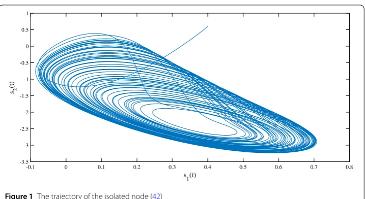
Figure 1The trajectory of the isolated node (42)
Example4.1 Consider the isolated node with both discrete and distributed delays:
⎧ c2= 0.5,c3= 0.5, and the inner-coupling matrices are given by
L1=
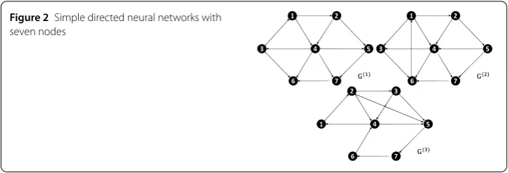
Figure 2Simple directed neural networks with seven nodes
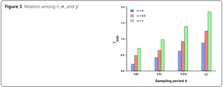
Table 1 Minimum allowable values ofγ for mixedH∞and passivity analysis satisfied with different values ofhandσ
γmin h= 0.05 h= 0.1 h= 0.15 h= 0.2
σ= 0 0.2124 0.4151 0.6210 0.8754
σ= 0.5 0.4831 0.6434 0.9212 1.2420
σ= 1 0.6967 0.9772 1.3864 1.8464
G(2)=
As presented in Fig.2, according to the pinned-node selection, nodes 1, 3, 4, 5, and 6 are chosen as controller. By applying our Theorem3.2, the relation among the parametersh, σ, andγ, are shown in Table1. Moreover, the histogram referring to the obtained relation is also plotted in Fig.3. Table2gives the maximum allowable sampling period ofhfor different values of. Thus, if we set = 0.3 andh= 0.5, then the gain matrices of the designed controllers will be obtained as follows:
Figure 3Relation amongh,σ, andγ
Table 2 Maximum allowable sampling period ofhin Example4.1
0.1 0.3 0.5 0.7 0.9
h 0.7543 0.6140 0.4814 0.3211 0.2034
Figure 4The trajectory of the isolated node (42) and network (1) with the time-varying scaling function
K6=
"
–1.4232 –0.2142 –0.1674 –2.0543 #
, K2=K7=
"
0 0
0 0
# .
Figure 5The state trajectory of the isolated nodeα(t)s(t) (42) and networkxi(t) (1)
Figure 6The EFPS error between isolate nodeα(t)s(t) (42) and networkxi(t) (1) without sample-data pinning
control (5)
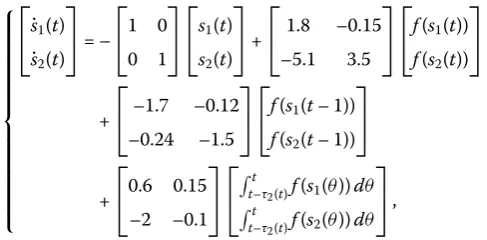
Example4.2 Consider the isolated node with both discrete and distributed delays:
⎧ ⎪ ⎪ ⎪ ⎪ ⎪ ⎪ ⎪ ⎪ ⎪ ⎪ ⎪ ⎪ ⎪ ⎨ ⎪ ⎪ ⎪ ⎪ ⎪ ⎪ ⎪ ⎪ ⎪ ⎪ ⎪ ⎪ ⎪ ⎩ ⎡ ⎣˙s1(t)
˙
s2(t)
⎤ ⎦= –
⎡ ⎣1 0
0 1
⎤ ⎦
⎡ ⎣s1(t)
s2(t)
⎤ ⎦+
⎡
⎣1.8 –0.15
–5.1 3.5
⎤ ⎦
⎡ ⎣f(s1(t))
f(s2(t))
⎤ ⎦
+ ⎡
⎣–1.7 –0.12
–0.24 –1.5
⎤ ⎦
⎡
⎣f(s1(t– 1)) f(s2(t– 1))
⎤ ⎦
+ ⎡
⎣0.6 0.15
–2 –0.1
⎤ ⎦ ⎡ ⎣
t
t–τ2(t)f(s1(θ))dθ
t
t–τ2(t)f(s2(θ))dθ
⎤ ⎦,
(43)
where f(si) =tanh(si(t)), (i= 1, 2),τ1(t) = 1+1e–t andτ2(t) = 1.2sin2(t). Then the
Figure 7The EFPS error between isolate nodeα(t)s(t) (42) and networkxi(t) (1) with sample-data pinning
control (5)
Figure 8The trajectory of the isolated node (43)
matrices are given by
L1=
"
1 0
0 1
#
, L2=
"
0.1 0
0 0.1
#
, L3=
"
0.1 0
0 0.1
# .
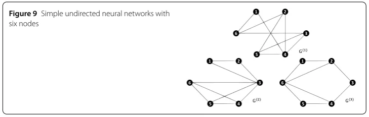
We consider the undirected NNs as shown in Fig.9, and the outer-coupling matrices are described by
G(1)= ⎡ ⎢ ⎢ ⎢ ⎢ ⎢ ⎢ ⎢ ⎢ ⎣
–2 0 0 1 0 1
0 –3 0 1 1 1
0 0 –3 1 1 1
1 1 1 –4 1 0
0 1 1 1 –3 0
1 1 1 0 0 –3
Figure 9Simple undirected neural networks with six nodes
Table 3 Maximum allowable sampling period ofhin Example4.2
0.1 0.3 0.5 0.7 0.9
h 0.8367 0.7134 0.5941 0.4723 0.3781
G(2)= ⎡ ⎢ ⎢ ⎢ ⎢ ⎢ ⎢ ⎢ ⎢ ⎣
–2 1 1 0 0 0
1 –2 1 0 0 0
1 1 –5 1 1 1
0 0 1 –3 1 1
0 0 1 1 –3 1
0 0 1 1 1 –3
⎤ ⎥ ⎥ ⎥ ⎥ ⎥ ⎥ ⎥ ⎥ ⎦ ,
G(3)= ⎡ ⎢ ⎢ ⎢ ⎢ ⎢ ⎢ ⎢ ⎢ ⎣
–2 1 0 0 0 1
1 –3 1 0 0 1
0 1 –2 1 0 0
0 0 1 –3 1 1
0 0 0 1 –2 1
1 1 0 1 1 –4
⎤ ⎥ ⎥ ⎥ ⎥ ⎥ ⎥ ⎥ ⎥ ⎦ .
As presented in Fig.9, according to the pinned-node selection, nodes 3, 4, and 6 are cho-sen as controller. Table3gives the maximum allowable sampling period ofhfor different values of. Thus, if we set = 0.3 andh= 0.5, then the gain matrices of the designed controllers will be obtained. Thus, if we set= 0.5 andh= 0.7, then the gain matrices of the designed controllers will be obtained as follows:
K3=
"
–3.2051 –1.3624 –2.3479 –2.7312 #
, K4=
"
–1.3465 –0.1384 –0.2478 –0.7543 #
,
K6=
"
–2.4312 –1.0065
–0.9431 –1.457
#
, K1=K2=K5=
"
0 0
0 0
# .
Figure 10 The trajectory of the isolated node (43) and network (1) with the time-varying scaling function
Figure 11 The state trajectory of the isolated nodeα(t)s(t) (43) and networkxi(t) (1)
Remark6 The networks in both examples of our study and the ones in the literature [21,
32,39] are different. In [21], the FPS of the network is achieved under pinning feedback controller design but the concerned network is still undirected. In [39], the conditions for pinning synchronization are suitable for directed network. In this paper, the pinning synchronization suitable for both directed and undirected networks. So, the considered networks are more general.
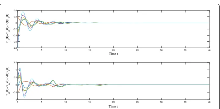
ef-Figure 12 The EFPS error between the isolate nodeα(t)s(t) (43) and networkxi(t) (1) without sample-data
pinning control (5)
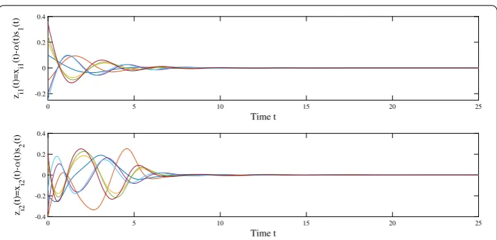
Figure 13 The EFPS error between the isolate nodeα(t)s(t) (43) and networkxi(t) (1) with sample-data
pinning control (5)
fectively save the communication bandwidth by only sending a necessary sampling signal through the network; see [42,43]. Nevertheless, considering the sampled-data controller and the digital form controller, which uses only the sampled information of the system at its instants, the important benefits in using a sampled-data controller are low-cost con-sumption, reliability, easy installation and being handy in real world problems.
5 Conclusions
In this paper, mixedH∞/passive EFPS of NNs with time-varying delays and hybrid
ex-amples are given to illustrate the effectiveness of the proposed theoretical results in this paper as well.
Funding
The first author was financially supported by the National Research Council of Thailand and Khon Kaen University 2019. The second author was supported by Rajamangala University of Technology Isan and the Thailand Research Fund (TRF), the Office of the Higher Education Commission (OHEC) (grant number MRG6180255). The third author was financial supported by Chiang Mai University. The fourth author was financially supported by University of Phayao. The fifth author was financially supported by Khon Kaen University.
Competing interests
The authors declare that they have no competing interests.
Authors’ contributions
All authors contributed equally to the writing of this paper. All authors read and approved the final manuscript.
Author details
1Department of Mathematics, Khon Kaen University, Khon Kaen, Thailand.2Department of Applied Mathematics and Statistics, Rajamangala University of Technology Isan, Nakhon Ratchasima, Thailand.3Department of Mathematics, Chiang Mai University, Chiang Mai, Thailand. 4Department of Mathematics, University of Phayao, Phayao, Thailand. 5Department of Statistics, Khon Kaen University, Khon Kaen, Thailand.
Publisher’s Note
Springer Nature remains neutral with regard to jurisdictional claims in published maps and institutional affiliations.
Received: 26 April 2019 Accepted: 8 August 2019 References
1. Cichocki, A., Unbehauen, R.: Neural Networks for Optimization and Signal Processing. Wiley, Hoboken (1993) 2. Cao, J., Wang, J.: Global asymptotic stability of a general class of recurrent neural networks with time-varying delays.
IEEE Trans. Circuits Syst. I50, 34–44 (2003)
3. Wang, J., Xu, Z.: New study on neural networks: the essential order of approximation. Neural Netw.23, 618–624 (2010)
4. Shen, H., Huo, S., Cao, J., Huang, T.: Generalized state estimation for Markovian coupled networks under round-robin protocol and redundant channels. IEEE Trans. Cybern.49, 1292–1301 (2019)
5. Alimi, A.M., Aouiti, C., Cherif, F., Dridi, F., M’hamdi, M.S.: Dynamics and oscillations of generalized high-order Hopfield neural networks with mixed delays. Neurocomputing321, 274–295 (2018)
6. Gu, K., Kharitonov, V.L., Chen, J.: Stability of Time-Delay System. Birkhauser, Boston (2003)
7. Seuret, A., Gouaisbaut, F.: Wirtinger-based integral inequality: application to time-delay systems. Automatica49, 2860–2866 (2013)
8. Maharajan, C., Raja, R., Cao, J., Rajchakit, G.: Fractional delay segments method on time-delayed recurrent neural networks with impulsive and stochastic effects: an exponential stability approach. Neurocomputing323, 277–298 (2019)
9. Zhao, N., Lin, C., Chen, B., Wang, Q.G.: A new double integral inequality and application to stability test for time-delay systems. Appl. Math. Lett.65, 26–31 (2017)
10. Maharajan, C., Raja, R., Cao, J., Rajchakit, G., Alsaedi, A.: Novel results on passivity and exponential passivity for multiple discrete delayed neutral-type neural networks with leakage and distributed time-delays. Chaos Solitons Fractals115, 268–282 (2018)
11. Zhang, X., Fan, X.F., Xue, Y., Wang, Y.T., Cai, W.: Robust exponential passive filtering for uncertain neutral-type neural networks with time-varying mixed delays via Wirtinger-based integral inequality. Int. J. Control. Autom. Syst.15, 585–594 (2017)
12. Cao, J., Chen, G., Li, P.: Global synchronization in an array of delayed neural networks with hybrid coupling. IEEE Trans. Syst. Man Cybern., Part B, Cybern.38, 488–498 (2008)
13. Huang, B., Zhang, H., Gong, D., Wang, J.: Synchronization analysis for static neural networks with hybrid couplings and time delays. Neurocomputing148, 288–293 (2015)
14. Selvaraj, P., Sakthivel, R., Kwon, O.M.: Finite-time synchronization of stochastic coupled neural networks subject to Markovian switching and input saturation. Neural Netw.105, 154–165 (2018)
15. Zhang, J., Gao, Y.: Synchronization of coupled neural networks with time-varying delay. Neurocomputing219, 154–162 (2017)
16. Yotha, N., Botmart, T., Mukdasai, K., Weera, W.: Improved delay-dependent approach to passivity analysis for uncertain neural networks with discrete interval and distributed time-varying delays. Vietnam J. Math.45, 721–736 (2017) 17. Fan, Y.Q., Xing, K.Y., Wang, Y.H., Wang, L.Y.: Projective synchronization adaptive control for different chaotic neural
networks with mixed time delays. Optik127, 2551–2557 (2016)
18. Yu, J., Hu, C., Jiang, H., Fan, X.: Projective synchronization for fractional neural networks. Neural Netw.49, 87–95 (2014) 19. Zhang, W., Cao, J., Wu, R., Alsaedi, A., Alsaadi, F.E.: Projective synchronization of fractional-order delayed neural
networks based on the comparison principle. Adv. Differ. Equ.2018(73), 1 (2018)
21. Shi, L., Zhu, H., Zhong, S., Shi, K., Cheng, J.: Function projective synchronization of complex networks with asymmetric coupling via adaptive and pinning feedback control. ISA Trans.65, 81–87 (2016)
22. Niamsup, P., Botmart, T., Weera, W.: Modified function projective synchronization of complex dynamical networks with mixed time-varying and asymmetric coupling delays via new hybrid pinning adaptive control. Adv. Differ. Equ. 2018(435), 1 (2018)
23. Samidurai, R., Rajavel, S., Zhu, Q., Raja, R., Zhou, H.: Robust passivity analysis for neutral-type neural networks with mixed and leakage delays. Neurocomputing175, 635–643 (2016)
24. Shen, H., Xing, M., Huo, S., Wu, Z.G., Park, J.H.: Finite-timeH∞asynchronous state estimation for discrete-time fuzzy Markov jump neural networks with uncertain measurements. Fuzzy Sets Syst.356, 113–128 (2019)
25. Raja, R., Zhu, Q., Samidurai, R., Senthilraj, S., Hu, W.: Improved results on delay-dependentH∞control for uncertain systems with time-varying delays. Circuits Syst. Signal Process.36, 1836–1859 (2017)
26. Song, S., Song, X., Balsera, I.T.: MixedH∞/passive projective synchronization for nonidentical uncertain
fractional-order neural networks based on adaptive sliding mode control. Neural Process. Lett.47, 443–462 (2018) 27. Mathiyalagan, K., Park, J.H., Sakthivel, R., Anthoni, S.M.: Robust mixedH∞and passive filtering for networked Markov
jump systems with impulses. Signal Process.101, 162–173 (2014)
28. Wu, Z.G., Park, J.H., Su, H., Song, B., Chu, J.: MixedH∞and passive filtering for singular systems with time delays. Signal Process.93, 1705–1711 (2013)
29. Selvaraj, P., Sakthivel, R., Marshal Anthoni, S., Mo, Y.C.: Dissipative sampled-data control of uncertain nonlinear systems with time-varying delays. Complexity21, 142–154 (2015)
30. Kumar, S.V., Anthoni, S.M., Raja, R.: Dissipative analysis for aircraft flight control systems with randomly occurring uncertainties via non-fragile sampled-data control. Math. Comput. Simul.155, 217–226 (2019)
31. Ma, C., Qiao, H., Kang, E.: MixedH∞and passive depth control for autonomous underwater vehicles with Fuzzy memorized sampled-data controller. Int. J. Fuzzy Syst.20, 621–629 (2018)
32. Rakkiyappan, R., Sakthivel, N.: Pinning sampled-data control for synchronization of complex networks with probabilistic time-varying delays using quadratic convex approach. Neurocomputing162, 26–40 (2015) 33. Wang, J., Su, L., Shen, H., Wu, Z.G., Park, J.H.: MixedH∞/passive sampled-data synchronization control of complex
dynamical networks with distributed coupling delay. J. Franklin Inst.254, 1302–1320 (2017)
34. Su, L., Shen, H.: MixedH∞/passive synchronization for complex dynamical networks with sampled-data control. Appl. Math. Comput.259, 931–942 (2015)
35. Song, Q., Cao, J.: On pinning synchronization of directed and undirected complex dynamical networks. IEEE Trans. Circuits Syst. I, Regul. Pap.57, 672–680 (2010)
36. Song, Q., Cao, J., Liu, F.: Pinning synchronization of linearly coupled delayed neural networks. Math. Comput. Simul. 86, 39–51 (2012)
37. Zhen, C., Cao, J.: Robust synchronization of coupled neural networks with mixed delays and uncertain parameters by intermittent pinning control. Neurocomputing141, 153–159 (2014)
38. Gong, D., Lewis, F.L., Wang, L., Xu, K.: Synchronization for an array of neural networks with hybrid coupling by a novel pinning control strategy. Neural Netw.77, 41–51 (2016)
39. Wen, G., Yu, W., Hu, G., Cao, J., Yu, X.: Pinning synchronization of directed networks with switching topologies: a multiple Lyapunov functions approach. IEEE Trans. Neural Netw. Learn. Syst.26, 3239–3250 (2015)
40. Zeng, D., Zhang, R., Liu, X., Zhong, S., Shi, K.: Pinning stochastic sampled-data control for exponential synchronization of directed complex dynamical networks with sampled-data communications. Neurocomputing337, 102–118 (2018)
41. Rakkiyappan, R., Latha, V.P., Sivaranjani, K.: ExponentialH∞synchronization of Lur’e complex dynamical networks using pinning sampled-data control. Circuits Syst. Signal Process.36, 3958–3982 (2017)
42. Wang, J., Chen, M., Shen, H., Park, J.H., Wu, Z.G.: A Markov jump model approach to reliable event-triggered retarded dynamic output feedback control for networked systems. Nonlinear Anal. Hybrid Syst.26, 137–150 (2017) 43. Shen, M., Pare, J.H., Fei, S.: Event-triggered nonfragile filtering of Markov jump systems with imperfect transmissions.