R E S E A R C H
Open Access
Joint maximum likelihood time-delay
estimation for LTE positioning in multipath
channels
José A del Peral-Rosado
1*, José A López-Salcedo
1, Gonzalo Seco-Granados
1, Francesca Zanier
2and Massimo Crisci
2Abstract
This paper presents a joint time-delay and channel estimator to assess the achievable positioning performance of the Long Term Evolution (LTE) system in multipath channels. LTE is a promising technology for localization in urban and indoor scenarios, but its performance is degraded due to the effect of multipath. In those challenging environments, LTE pilot signals are of special interest because they can be used to estimate the multipath channel and counteract its effect. For this purpose, a channel estimation model based on equi-spaced taps is combined with the time-delay estimation, leading to a low-complexity estimator. This model is enhanced with a novel channel parameterization able to characterize close-in multipath, by introducing an arbitrary tap with variable position between the first two equi-spaced taps. This new hybrid approach is adopted in the joint maximum likelihood (JML) time-delay estimator to improve the ranging performance in the presence of short-delay multipath. The JML estimator is then compared with the conventional correlation-based estimator in usual LTE conditions. These conditions are characterized by the extended typical urban (ETU) multipath channel model, additive white Gaussian noise (AWGN) and LTE signal bandwidths equal to 1.4, 5 and 10 MHz. The resulting time-delay estimation performance is assessed by computing the cumulative density function (CDF) of the errors in the absence of noise and the root-mean-square error (RMSE) and bias for signal-to-noise ratio (SNR) values between−20 and 30 dB.
Keywords: LTE; Positioning; OFDM modulation; Positioning Reference Signal (PRS); Multicarrier signal; Multipath channel modelling; Joint time-delay and channel estimation; Ranging
1 Introduction
Navigation and positioning technologies are every day more important in civil applications, demanding enhance-ments on accuracy, availability and reliability. Position-ing improvements are mainly achieved, thanks to the advances in Global Navigation Satellite Systems (GNSS) and the introduction of new systems, such as Galileo. However, a myriad of possible working conditions are faced in ubiquitous positioning, where the GNSS nom-inal performance is highly degraded, such as in urban environments or indoors. Thus, the use of complemen-tary terrestrial localization systems is envisaged as a major step towards the realization of anywhere and anytime
*Correspondence: [email protected]
1Department of Telecommunications and Systems Engineering, Universitat Autònoma de Barcelona (UAB), Q Building, Cerdanyola del Vallès 08193, Spain Full list of author information is available at the end of the article
positioning. A relevant example of these technologies is the Long Term Evolution (LTE), a next-generation mobile communications system with promising perspectives on positioning. Indeed, the LTE standard [1,2] specifies a dedicated downlink reference signal for observed time difference of arrival (OTDoA) localization, i.e. the posi-tioning reference signal (PRS). The LTE OTDoA method is based on the time-delay estimation (TDE) of the signals received from different source transmitters (i.e. cellular base stations). Since the LTE downlink signal is based on the orthogonal frequency division multiplexing (OFDM) modulation, the TDE is typically performed with the LTE pilot subcarriers in the frequency domain. Using this method, recent research studies, such as those in [3-5], have shown the potential of LTE to provide accurate posi-tioning. However, multipath propagation and non-line-of-sight conditions are still the main limiting factors in urban
environments, once inter-cell interference is removed. Therefore, countermeasures against multipath are needed in order to achieve the ultimate positioning performance in LTE.
In order to properly understand and mitigate the effect of multipath, it is important to have a good character-ization of the propagation conditions and reflect them on the estimation model of the receiver. Many channel models have been proposed to characterize the propa-gation conditions of the possible LTE working scenarios. Among them, the LTE standard adopted an extension of the tapped-delay line (TDL) channel models specified for the second- and third-generation mobile systems, i.e. Global System for Mobile communications (GSM) and Universal Mobile Telecommunications System (UMTS). One of these propagation models is the extended typical urban (ETU) model, described in Annex B of [6] and [7]. The ETU model is of special interest because it defines a power-delay profile (PDP) with a line-of-sight (LoS) sig-nal more attenuated (in average) than the multipath rays. This is a representative example of harsh conditions where LTE is expected to be used. In these conditions, the rang-ing performance of the correlator or matched filter is relatively poor [8]. The correlation-based TDE can be con-sidered as a conventional time-delay estimation method due to its low complexity, being the maximum likelihood (ML) estimator in additive white Gaussian noise (AWGN) channels. However, in multipath channels, the delayed reflections of the signal induce a notable bias on this con-ventional estimation. Thus, another estimator is required in order to improve the TDE performance in multipath environments.
The time-delay estimation can be enhanced by model-based estimators. These estimators use channel estima-tion models in order to counteract the effect of multipath. The aim of these models is to characterize the response of the channel, instead of identifying the physical mul-tipath components of the specific environment. There are many possibilities for these channel estimation mod-els. On the one hand, the most accurate model corre-sponds to the estimation of amplitude, phase and delay of every propagation ray. However, it is also the most com-plex model because of the many unknowns to estimate. Despite its complexity, this estimation model has been widely studied, for instance, with super-resolution tech-niques in [9,10], with the ML criterion in [11], or in a two-step approach in [12]. On the other hand, channel estimation models can be simplified by defining equi-spaced or periodic taps relative to the time delay of the first path. Since this model is based on the uniform sampling of the channel, it has been used with the com-pressed sampling theory for channel estimation, such as in [13,14], but it can also be found in multipath interference cancellation [15].
Timing synchronization for data transmission does not need to achieve the extreme accuracy required for posi-tioning. This is the reason why, in communication appli-cations, the ML approach is widely applied to channel estimation assuming the time delay to be coarsely cor-rected in a previous stage, and the residual time delay is considered negligible. There are still some contributions that propose the joint maximum likelihood (JML) esti-mation of the time delay and channel response in OFDM systems, considering a model based on equi-spaced or periodic taps, but few of them deal with the specific case of ranging applications. The authors of [16] propose an algorithm based on the JML approach and on the chan-nel length estimation, but providing only coarse timing estimates. In [17], two JML estimators are applied for syn-chronization of multiple users. The first one is a joint frequency and channel estimator, while the second one is a joint time-delay and channel estimator. A similar JML approach is used for ranging purposes considering an IEEE 802.16 system [18]. An approximation of the JML algorithm is proposed in [19] using early and late estima-tions in a delay lock loop (DLL). The JML estimation has also been studied for multicarrier ranging considering the optimal placement of pilot subcarriers in [20] and applied without data-aiding after the definition of a unified signal model in [21]. In addition, a very preliminary study of the JML in LTE for a very specific scenario is presented in [22]. Therefore, the joint estimation algorithms found in the literature have mainly focused on communication applica-tions, where a very accurate time-delay estimation is not critical in general. In our ranging application, the repre-sentation of the channel has to be improved, especially for those scenarios where multipath highly deteriorates the time-delay estimation. Thus, the channel estimation models have to be adapted to these harsh environments.
approach, is studied in this paper and used to assess the achievable positioning performance of LTE, considering a low-complexity time-delay estimation that exploits the structure of the LTE OFDM signals. This estimation is analyzed for usual working conditions, represented by typical LTE signal bandwidths with the ETU standard channel model.
The remainder of this paper is organized as follows. Section 2 defines the signal model and describes the main LTE pilot signals. Section 3 defines the propagation chan-nel model. Section 4 reviews the different chanchan-nel estima-tion models and derives the joint ML estimator, including the novel channel parameterization. In Section 5, the per-formance of the joint ML estimators is assessed with numerical results in multipath and noise channels for dif-ferent signal bandwidths. Finally, conclusions are drawn in Section 6.
2 Signal model
The downlink transmission of the LTE mobile com-munications standard is based on the OFDM modula-tion, whose complex-valued baseband representation is given by:
where C is the power of the band-pass signal,N is the total number of subcarriers,b(n)is the complex-valued symbol transmitted at the nth subcarrier, and T is the
OFDM symbol period. The symbol b(n) is defined by
b(n) = d(n)·p(n), beingd(n)the data or pilot symbol assigned with a relative power weightp(n)2, which is con-strained byNn=−01p(n)2=N. In particular, the downlink physical layer of the LTE specification [1] defines a symbol periodT of 66.67µs, which corresponds to a subcarrier spacingFsc = 1/T of 15 kHz. The transmission grid is defined in time and frequency by resource blocks (RB), which are the minimum resource allocation unit formed by seven OFDM symbols and 12 subcarriers in the normal cyclic prefix configuration. The system bandwidth is scal-able from 1.4 to 20 MHz, but the guard bands are left at the edges of the spectrum; thus, only a minimum transmis-sion bandwidth of 6 RB (i.e. 1.08 MHz) and a maximum of 100 RB (i.e. 18 MHz) can be configured [6].
Assuming the successful removal of the cyclic prefix and perfect carrier frequency synchronization, the baseband received signal is
yc(t)=xc(t)∗hc(t)+nc(t), (2)
where∗is the convolution operation,hc(t)is an unknown channel impulse response (CIR), andnc(t) is the white Gaussian noise. If the LTE receiver applies a sampling
frequencyFs, defined by the sampling periodTs =1/Fs=
T/N, the discrete-time signal model is
xd(m)=. xc(mTs)= tistically uncorrelated withnd(m) ∼ N
applying anN-point discrete Fourier transform (DFT) to
yd(m), we have
r(n)=√2C·b(n)·H(n)+w(n), (4)
where n is the index of the subcarriers, H(n) =
F{hd(m)}is the channel frequency response, beingF{·} the discrete Fourier transform operator, andw(n)are the noise frequency samples, which are statistically uncorre-lated withw(n)∼N0,σw2.
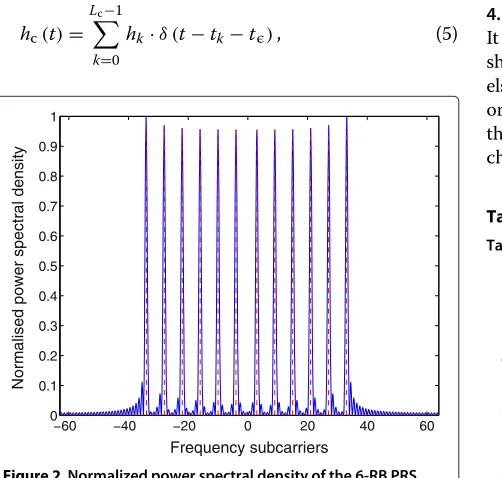
The LTE pilot signals are constituted by the synchro-nization signals and the reference signals. The primary and secondary synchronization signals (i.e. PSS and SSS, respectively) are allocated in the centre of the spectrum with 62 contiguous pilot subcarriers, and avoiding the DC subcarrier. On the other hand, the reference signals, such as the cell-specific reference signal (CRS), are scattered in time and frequency spanning the maximum bandwidth of the configuration under use. Among the different pilot signals, the PRS is of special interest because its coordi-nated transmission avoids the inter-cell interference from neighbour cells, which is produced due to the single-frequency transmission. The pilot distribution of the CRS and PRS is shown in Figure 1. It should be noticed that the total number of subcarriersNdefined in the signal model is equivalent to the bandwidth occupied by the active sub-carriers, i.e. effective bandwidth. Using only the reference signals, the equivalent bandwidth is defined byN = 12·
NRB−4, whereNRBis the number of resource blocks. As an example, let us consider that 6 RB and uniform power distribution among pilots subcarriers are used. Then, the normalized power spectral density of one PRS symbol without data transmission is shown in Figure 2. The total number of subcarriersNis equal to 68 subcarriers, which is equivalent to the effective bandwidth.
3 Propagation channel model
Figure 1Time and frequency distribution of the LTE CRS and PRS pilots.
second- and third-generation mobile communications, i.e. GSM and UMTS, which are extended to cover the wide bandwidths of LTE signals. Following the TDL model, the propagation channel model shown in (2) is defined as
hc(t)= Lc−1
k=0
hk·δ (t−tk−t), (5)
−60 −40 −20 0 20 40 60
0 0.1 0.2 0.3 0.4 0.5 0.6 0.7 0.8 0.9 1
Frequency subcarriers
Normalised power spectral density
Figure 2Normalized power spectral density of the 6-RB PRS without data transmission.
whereLcis the number of taps of the channel,hk is the complex gain for thekth path,δ (t) is the Dirac delta,tk is the tap delay relative to the first tap (i.e.t0 = 0), and
t is the time delay introduced by the channel (i.e. the time delay of the first arriving ray). The power-delay pro-file of the LTE TDL models is defined in Annex B of [6] and [7], by specifying the fixed delaytk and relative aver-age power RPk for every tap. The channel coefficientshk of these extended models are time-varying with a Rayleigh distribution, and following a classical Jakes Doppler spectrumS(f),
S(f)∝ 1
1−f/fD2
, for f ∈−fD,fD, (6)
beingfDthe maximum Doppler shift. Among these
mod-els, our interest is focused on the ETU channel model, whose parameters are shown in Table 1. As it can be noticed, the ETU model is characterized by a large delay spread of 5µs and strong multipath rays. Thus, the max-imum average energy of the CIR may be located far from the time delay of the first arriving path. This deviation causes a notable degradation on the performance of the conventional TDE. The reason is that the matched fil-ter estimates the time delay based on the maximum peak of the correlation, which coincides with the maximum energy of the CIR. Since the strongest correlation peak may not correspond to the first arriving path, a bias is produced on the time-delay estimation. Therefore, the ETU model defines a harsh environment, where the per-formance of the conventional estimator is relatively poor.
4 Time-delay estimation
4.1 Channel estimation models
It is important to note that channel estimation models should be distinguished from propagation channel mod-els. The first ones consider the response of the channel in order to later counteract its effect. The second ones model the physical channel to understand the behaviour of the channel itself. Thus, the propagation channel models are
Table 1 ETU channel model parameters
Tapk tk(ns) RPk(dB)
1 0 −1.0
2 50 −1.0
3 120 −1.0
4 200 0.0
5 230 0.0
6 500 0.0
7 1,600 −3.0
8 2,300 −5.0
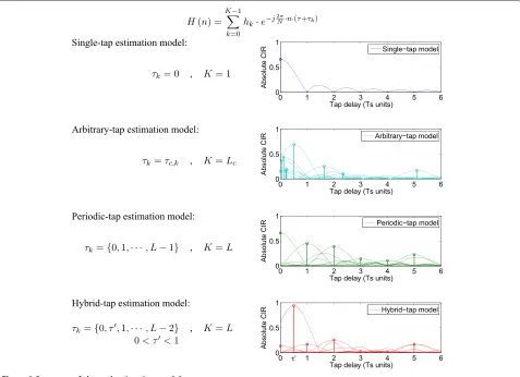
used to simulate the actual channel, while the channel estimation models are used to represent the effect of the channel on the time-delay estimation. Next, we describe those channel estimation models that are typically used, as well as a new model presented in this work.
4.1.1 Single-tap model
The most simple and used channel estimation model is the single-tap model. It assumes that the signal is just atten-uated and delayed by the channel. Thus, this estimation model is only defined by a single-channel coefficienth0, which can be complex-valued, associated to the propaga-tion time delayt. Using a bandlimited representation for the channel, the discrete CIR of this model is
hST(m)=h0·sinc(m−τ), (7)
where sinc(x) = sinπ(π·x·x) is the sinc function, and τ =.
t/Ts is the discrete-time symbol-timing error, which is the time delay to estimate. This estimation model is typ-ically applied in AWGN channels. Using this model, the derivation of the ML estimator results in the correlation-based estimator. As it was discussed at the end of
Section 3, this conventional TDE has a considerable bias in multipath channels. The main characteristics of this channel model are shown in Figure 3.
4.1.2 Arbitrary-tap model
The most accurate model is constituted by the amplitude, phase and delay of every physical multipath ray. However, this model is also the most complex because these param-eters have to be estimated for every tap. Since the taps’ delays are in positions to be determined, this model is hereafter called the arbitrary-tap model. Its discrete CIR is written as
hAT(m)= L−1
k=0
hk·sinc(m−τk−τ), (8)
whereL is the number of taps,hk is the channel coeffi-cient for the kth tap, τk is the relative delay to the first tap (i.e. τ0 = 0), and τ is the time delay. As it shown in Figure 3, the arbitrary-tap model is represented, in that case, by matching the Lc propagation taps at delay positionsτc,k. Although the channel response can be accu-rately reconstructed using this model, the implementation
complexity is a major concern. For instance, the number of unknowns substantially increases (withouta priori statis-tics) in dense multipath due to the high number of rays to estimate. Thus, the iterative methods implemented for the TDE, such as super-resolution techniques [10], have a high computational burden.
4.1.3 Periodic-tap model
The complexity of the channel estimation model is reduced by placing the estimation taps in equi-spaced or periodic delay positions. The aim is to avoid the tap delay estimation for every physical ray and focus on the prop-agation time-delay estimation. Thus, the actual physical tap positions are not estimated, and the resulting model is a sampled version of the channel impulse response. The discrete CIR of the periodic-tap model is
hPT(m)= L−1
k=0
hk·sinc(m−k−τ), (9)
where Lis the number of taps,hk is the channel coeffi-cient for thekth tap, andτ is the time delay. Ideally, the sampled model would require an infinite number of taps in order to perfectly represent the channel. The solution described in (9) is to truncate the number of taps toL, by assuming that the rest of taps have a negligible contribu-tion. However, this assumption may produce an incorrect characterization of the channel response, leading to the so-called problem of model mismatch. The periodic-tap model is represented in the example of Figure 3 consid-ering six taps. Since the tap positions are assumed to be equi-spaced, the close-in multipath, i.e. multipath close to the LoS signal, is not properly modelled when it appears between the first two samples at delay 0 andTs. Thus, the multipath energy missed between samples may severely degrade the performance of the time-delay estimation. In the opposite case, if the sampling periodTs is small
enough, the number of taps L has to expand a similar
interval to the multipath dispersion. The design ofL is beyond the scope of the paper, but it can be obtained by means of model order selection techniques, such as minimum description length (MDL) or Akaike [16], or by considering the delay spread of the channel, which can be estimated as in [24] and the references therein.
4.1.4 Hybrid-tap model
A novel hybrid solution is proposed in this paper by using the equi-spaced taps together with an additional tap in a position to be determined between the first two. Thus, the equi-spaced taps allow the estimator to capture most of the multipath energy present in the propagation model, while the additional tap models close-in multipath with only the added complexity of having one more variable. The CIR of the hybrid-tap model is defined as
hHT(m)=
whereLis the number of taps,hkis the channel coefficient for thekth periodic tap, hL−1andτdenote the channel coefficient and delay of the arbitrary tap, respectively, and τ is the time delay. As an example, the hybrid-tap model is represented in Figure 3, where the arbitrary-tap delay values ofτare fixed within 0 and 1 with respect toτ.
4.2 One-dimensional joint ML estimator
In order to derive a low-complexity time-delay estimator, the periodic-tap model is first selected. Thus, the esti-mation parameters are the time delayτ and the channel coefficientsh = [h0,· · ·,hL−1]T. The received signal of (4) can be rewritten in matrix notation as in [20-22],
r=BτFLh+w, (11)
andFL is composed of the firstL columns of the
zero-frequency-centredN×NDFT matrix,
FL=
Hence, the received signal is expressed as
r=Aτh+w. (19)
Given this formulation, the maximum likelihood criterion is applied, which results in
where (r;τ,h)is the likelihood function of the received
samples parameterized by the unknownsτ andh, which
is defined by a multivariate Gaussian distribution,
(r;τ,h)=C0exp
being C0 an irrelevant constant. Substituting the log-likelihood function in (20) leads to the following mini-mization problem:
which coincides with the nonlinear least squares (NLS) criterion, sinceτdepends nonlinearly on the received sig-nal model. The resulting two-dimensiosig-nal optimization can be separated by minimizing first with respect tohand then with respect toτ as in [25], which can be written as
ˆ
Then, the well-known least-squares solution can be applied to obtain the ML estimate of the unknown channel coefficients as
ˆ h=A†
τr, (24)
whereA†τ denotes the Moore-Penrose pseudo-inverse of
Aτ, which is defined as
being the superindexH the Hermitian conjugate. Intro-ducing the least-squares solution into (23), the ML esti-mation of the time delay results in
ˆ projection matrix onto the subspace orthogonal to that spanned by the columns ofAτ. Thus, the decoupling ofτˆ andhˆ leads to the proposed ML time-delay estimator of (26). It is hereafter calledone-dimensional joint ML( 1D-JML) time-delay and channel estimator. The 1D-JML esti-mation is computed numerically by minimizing the cost function ofP⊥A,τr2as a function ofτ. This optimization is not complex because it is a one-dimensional function that is simply evaluated within the range [−1/2, 1/2] and then minimized. This range is defined to find the residual time delay after a coarse estimation. The minimum could be obtained by solving the function with a sufficiently
fine grid of points. However, the fminbndfunction of
MATLAB is used for an efficient computation, which finds the minimum in the search interval. Instead of doing
an exhaustive evaluation, this function searches the min-imum by means of the golden section technique followed by a parabolic interpolation.
Let us study the particular case ofLequal to 1. In this case, the channel is formed only by one ray, thusAτ is a
N×1 matrix defined asAτ =BτF1. Developing further the expression of (26), the one-dimensional optimization problem results into the following maximization of the cost function:
whereR(τ)is the cross-correlation of the received signal
rwith the pilot symbolsbdefined in the scalar notation as
R(τ)=
Thus, the particular case of the 1D-JML estimation for
L= 1 reduces to the estimation based on the correlation or matched filter output. This confirms the optimality of the matched filter for time-delay estimation in the absence of multipath.
4.3 Two-dimensional joint ML estimator
The derivation of the JML estimator, using the periodic-tap channel estimation model described in (9), results in a low-complexity implementation by decoupling the prob-lem of joint time-delay and channel estimation. Now, the hybrid-tap estimation model of (10) is applied to enhance the characterization of the physical channel response. Using this novel channel parameterization, the model mismatch is reduced at the expense of adding one more estimation parameter, the arbitrary-tap delayτ. Consid-ering the derivation of the 1D-JML obtained in (26), the problem at hand is solved following the same procedure.
This leads to the two-dimensional joint ML (2D-JML)
estimator, which can be expressed as
The two-dimensional optimization of (29) is
com-puted by an exhaustive search in the τ × τ region of
[−1/2, 1/2]×[0, 1]. Since the cost function ofPA⊥,τ,τr2
only depends on two parameters, its minimum can be found with the required accuracy by evaluating the func-tion in a sufficiently fine grid of points.
5 Numerical results
The proposed JML time-delay estimator is, in principle, applicable to any multicarrier signal. Multicarrier signals show a flexible allocation of data and pilot resources that facilitates the adoption of the JML estimator. Thus, the JML estimator is used to show the achievable performance with the LTE positioning reference signals for different signal bandwidths. The TDE performance of the 1D- and 2D-JML estimators for L > 1 is compared with that of
the 1D-JML estimator for L = 1, i.e. the conventional
correlation-based technique. First, the multipath error envelope (MPEE) is used to characterize the multipath impact on the TDE. Second, the bias and the root-mean-square error (RMSE) of the JML estimators is statistically assessed over realistic multipath and noise conditions. In order to conduct these analyses, the OFDM signal is assumed to be successfully acquired, being the receiver in signal tracking mode, thus the time-delay estimation range is defined within [−Ts/2,Ts/2], or [−1/2, 1/2] since τ is inTsunits.
5.1 Multipath error envelope
The main properties of the proposed estimator can be studied through the MPEE. This metric evaluates the impact of a two-ray multipath model on the time-delay estimation. In the absence of noise, the MPEE represents the time-delay error produced by a multipath reflection (with specific delay, power and phase) when it is added to the LoS component. Thus, the received signal in the MPEE analysis is defined as
yd(m)=xd(m−τ)+a1·ejφ1 ·xd(m−τ−τ1), (31)
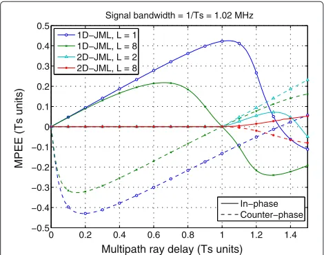
where a1, φ1 andτ1 are the amplitude, phase and delay of the multipath ray, respectively. The MPEE is computed considering−1 dB of relative power to the LoS ray within a delay range between 0 and 3·Ts/2. The multipath ray is added constructively and destructively to the LoS com-ponent, i.e. the multipath contribution is in-phase (i.e. φ1 = 0) and counter-phase (i.e. φ1 = π), respectively. In this scenario, the LTE PRS is configured for the low-est bandwidth of 6 RB, assuming no data allocation on the transmitted symbol. As it is discussed in Section 2, the 6-RB PRS bandwidth is defined byN=12·NRB−4=68 subcarriers, which results inTs=T/N=980.39 ns and a signal bandwidth equal to 1/Ts=1.02 MHz.
The resulting MPEE is shown in Figure 4, by comparing the 1D-JML estimator forL= {1, 8}with the 2D-JML esti-mator forL= {2, 8}, using expressions (27), (26) and (29), respectively. As it can be noticed, the multipath errors are normalized with respect to the sampling periodTs. It has been confirmed through simulations that the same rel-ative results are obtained for higher signal bandwidths.
Thus, the maximum errors maxof the 1D-JML estimator
are calculated in metres for constructive and destructive cases using different sampling periods, as it is shown in Table 2. Three main results can be identified:
• The effect of increasing the number of taps from L=1toL=8in the 1D-JML estimator, that is, from using a single-tap model to a periodic-tap model, improves the TDE performance, but there is still a significant bias in both cases.
• While the 1D-JML estimator forL= {1, 8}is only unbiased at certain instants (e.g.τ = {1.34, 1}, respectively), the 2D-JML estimator is completely unbiased for values of multipath delayτ1within 0 and 1 due to the matching between the channel estimation model and the propagation channel model.
• The effect of decreasing the number of taps from L=8toL=2in the 2D-JML estimator does not have the same behaviour as in the 1D-JML estimator because the hybrid approach is still unbiased for values of multipath delayτ1within 0 and 1.
5.2 Bias and RMSE of the JML estimators over realistic conditions
The multipath error envelope has shown the bias intro-duced by a particular multipath ray on the time-delay esti-mation. The results indicate the potential of the new JML
0 0.2 0.4 0.6 0.8 1 1.2 1.4 −0.5
−0.4 −0.3 −0.2 −0.1 0 0.1 0.2 0.3 0.4 0.5
Multipath ray delay (Ts units)
MPEE (Ts units)
Signal bandwidth = 1/Ts = 1.02 MHz
1D−JML, L = 1 1D−JML, L = 8 2D−JML, L = 2 2D−JML, L = 8
In−phase Counter−phase
Table 2 Maximum TDE errors of the 1D-JML in the MPEE
max,L=1(m) max,L=8(m)
Bandwidth (RB) Ts/2 (m) φ1=0 φ1=π φ1=0 φ1=π
6 147.06 127.02 −127.07 64.71 −96.11
25 33.78 29.18 −29.19 14.87 −22.08
50 16.78 14.49 −14.50 7.38 −10.97
approach to improve the TDE performance with respect to the conventional correlator-based estimator. However, the two-ray multipath model does not represent general urban channels. Thus, the ETU channel model is used to assess the performance of the estimators in more realistic conditions.
5.2.1 Low signal bandwidth (i.e. 1.4 MHz)
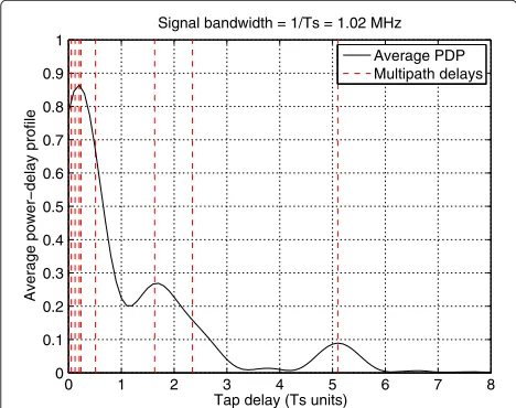
The effect of multipath on the time-delay estimation is first assessed statistically considering the ETU model and the lowest LTE bandwidth of 1.4 MHz. Within this band-width, the PRS is allocated along 6 RB without data transmission, which results in a signal bandwidth equal to 1/Ts = 1.02 MHz. For this case, 1,000 ETU realizations are computed with a Doppler shift of 500 Hz. The result-ing channel is represented with the average power-delay profile PDP in Figure 5. The average PDP is calculated with the mean absolute value of the discrete CIR for every th realizationh(m)in the interval [τ,τ +8], that is,
PDP(m)= 1 N·
N−1
=0
|h(m)|2, τ <m< τ+8, (32)
where N is the number of realizations. In Figure 5,
the multipath delays of the channel are highlighted with
0 1 2 3 4 5 6 7 8
0 0.1 0.2 0.3 0.4 0.5 0.6 0.7 0.8 0.9 1
Tap delay (Ts units)
Average power−delay profile
Signal bandwidth = 1/Ts = 1.02 MHz
Average PDP Multipath delays
Figure 5Average power-delay profile for ETU model with a 6-RB PRS bandwidth.One thousand channel realizations are used.
vertical red lines. As it can be seen, this channel model is mainly characterized by the presence of LoS signal and strong multipath in short delays. Thus, most of the multi-path energy is concentrated for delays between 0 andTs/2,
approximately. In addition, it can be seen (as specified in Table 1) that the delay spread of the ETU model is equal to 5.1·Ts. Then, if the periodic-tap estimation model is used, one can notice as the estimation taps at positions larger than the delay spread have a negligible multipath contribution. Thus, we use this prior information in order to correctly assume the truncation of the number of taps to the delay spread of the ETU model, which in the
1D-JML estimator corresponds toL = 6 and in the 2D-JML
estimator corresponds to L = 7. Using a higher
num-ber of taps, the estimators do not capture more channel energy, thus they may obtain a similar TDE performance (in absence of noise).
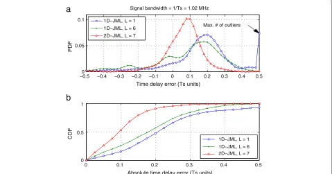
Given the generated ETU channel, time-delay errors are computed in the absence of AWG noise using the 1D- and 2D-JML estimators. The probability density func-tion (PDF) of the resulting time-delay errors is shown in Figure 6a. The performance of the 1D-JML estima-tor forL = 1 is poor, producing the highest number of outliers. The outlier estimations are defined as those time-delay estimations with an absolute error higher or equal toTs/2, which are then truncated toTs/2. In this sense, the application of the periodic-tap estimation model (with six taps) reduces the number of outliers. Nevertheless, the low sampling rate avoids this channel estimation model to properly characterize close-in multipath. Thus, using the new hybrid-tap estimation model, an additional arbi-trary tap is introduced between 0 andTs to reduce the model mismatch. The resulting 2D-JML estimator shows a notable improvement with respect to the 1D-JML esti-mators. This enhancement is highlighted by the cumu-lative density function (CDF) of the absolute time-delay error, shown in Figure 6b. For instance, the 2D-JML
esti-mator for L = 7 produces an absolute TDE error of
0.12·Ts(i.e. 35.3 m) for 67% of the cases, while the 1D-JML estimators obtain (for the same percentage of the cases) an error of 0.25·Ts(i.e. 73.5 m) withL= 1 and 0.23·Ts(i.e. 67.7 m) withL=6. Thus, the 2D-JML estimator provides an important reduction of the multipath error.
Once the impact of multipath has been assessed, AWG noise is added to the ETU channel model. The signal-to-noise ratio (SNR) takes values between−20 and 30 dB. For each SNR value, 1,000 ETU model realizations are processed. The time-delay errors (including the truncated outliers) obtained by the JML estimators for every SNR are used to compute the root-mean-square error, defined as
RMSE(τ )ˆ =
Eτˆ−τ2
−0.50 −0.4 −0.3 −0.2 −0.1 0 0.1 0.2 0.3 0.4 0.5 0.05
0.1
Time delay error (Ts units)
Signal bandwidth = 1/Ts = 1.02 MHz
Max. # of outliers
0 0.1 0.2 0.3 0.4 0.5
0 0.5 1
Absolute time delay error (Ts units)
CDF
1D−JML, L = 1 1D−JML, L = 6 2D−JML, L = 7
1D−JML, L = 1 1D−JML, L = 6 2D−JML, L = 7
a
b
Figure 6Performance of 1D- and 2D-JML estimators using ETU model without noise and 6-RB PRS bandwidth.(a)Probability density function of the time-delay estimations.(b)Cumulative density function of the time-delay estimations. One thousand channel realizations are used.
and the bias, expressed as
b(τ)ˆ =Eτˆ−τ, (34)
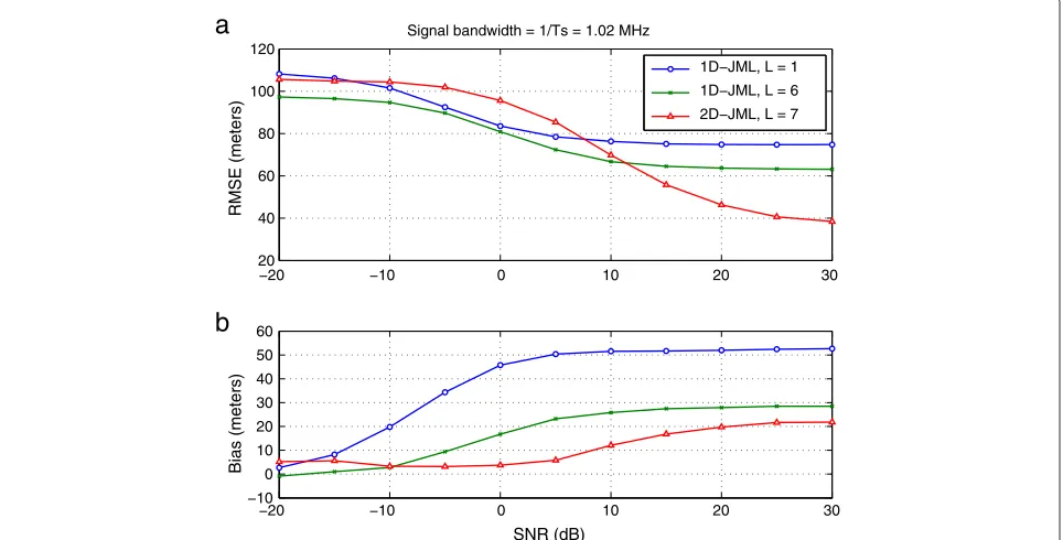
being E [·] the expectation operator. Considering both multipath and noise, the RMSE of the estimators is depicted in Figure 7a, whereas the bias of the estimators is shown in Figure 7b, being both metrics expressed in metres. Since the multipath channel changes every ETU realization, the RMSE and bias are not equal for high SNR. The lowest bias, i.e. 21.7 m, is achieved by the
2D-JML estimator forL = 7 at high-SNR values, such
as 30 dB. It obtains a major improvement with respect to the 1D-JML estimator forL= 1 (i.e. conventional TDE), whose minimum bias is equal to 52.7 m. In addition, the new hybrid estimation reduces the model mismatch error, since the 1D-JML estimator forL = 6 has a bias of 28.6 m at 30 dB of SNR. Nevertheless, the 2D-JML estima-tor is more affected by noise than the 1D-JML estimaestima-tors, which results in a higher RMSE at low SNR values. This is due to the fact that the variance of the joint ML estima-tion increases with the number of unknown parameters to estimate. Thus, there is a trade-off between the efforts to counteract multipath and the robustness against noise.
5.2.2 Typical signal bandwidths (i.e. 5 and 10 MHz)
The most usual working modes of LTE are based on the 5 and 10 MHz operating bandwidths. These configura-tions can be identified as typical modes because they are specified for most of the LTE bands, as it is shown in
Table 5.6.1-1 of [6]. The signal bandwidths associated to these modes are 25 RB (i.e. 4.5 MHz) and 50 RB (i.e. 9 MHz), respectively. Thus, the ETU model is applied with these typical bandwidths in order to represent usual LTE positioning conditions.
Using the ETU model realizations of the previous section, the average PDP is shown for both bandwidths in Figure 8. The range of the tap delay is defined between 0 and 1.96µs, which coincides with 2·Tsfor a 6-RB band-width. For the current bandwidths, the sampling period
Tsis 225 ns for 25 RB and 112 ns for 50 RB, given a total
number of N subcarriers equal to 296 and 596,
respec-tively. Thus, the time-delay estimation can be focused on the short-delay multipath. Given a higher channel band-width, the contribution of every multipath ray is more independent. In the same way, the sampling rate of the estimation model is higher, and more multipath energy can be captured by every estimation tap. Therefore, the 1D- and 2D-JML estimators can use a number of taps
Llower than the delay spread of the channel. For a 25-RB
bandwidth, we should consider L = 8 for the 1D-JML
estimator and L = 9 for the 2D-JML estimator, while
for a 50-RB bandwidth, we should consider L = 4 for
the 1D-JML estimator and L = 5 for the 2D-JML
esti-mator. A priori information of the average PDP should
be used to minimize the number of taps L according
−20 −10 0 10 20 30 20
40 60 80 100 120
a
b
RMSE (meters)
Signal bandwidth = 1/Ts = 1.02 MHz
−20 −10 0 10 20 30
−10 0 10 20 30 40 50 60
SNR (dB)
Bias (meters)
1D−JML, L = 1
1D−JML, L = 6
2D−JML, L = 7
Figure 7Performance of 1D- and 2D-JML estimators using ETU model with AWGN and 6-RB PRS bandwidth.(a)Root-mean-square error of the time-delay estimations.(b)Bias of the time-delay estimations. One thousand ETU model realizations per SNR are used.
The cumulative density function of the TDE errors obtained with the 1D- and 2D-JML estimators is com-pared using both bandwidths in Figure 9. As it can be seen, the 1D- and 2D-JML estimators forL > 1 improve the TDE performance with respect to the 1D-JML estimator forL=1 in both cases. In particular, there is a higher gain for 25-RB bandwidth than for 50-RB bandwidth. This is due to the fact that the estimation tap delays are changed with the sampling period. The best TDE performance is achieved when the estimation taps capture most of the multipath energy. In the cases under study, the periodic-tap 1D-JML estimator forL > 1 performs slightly better
than the hybrid-tap 2D-JML estimator forL > 1. How-ever, both estimators still achieve a very accurate ranging performance.
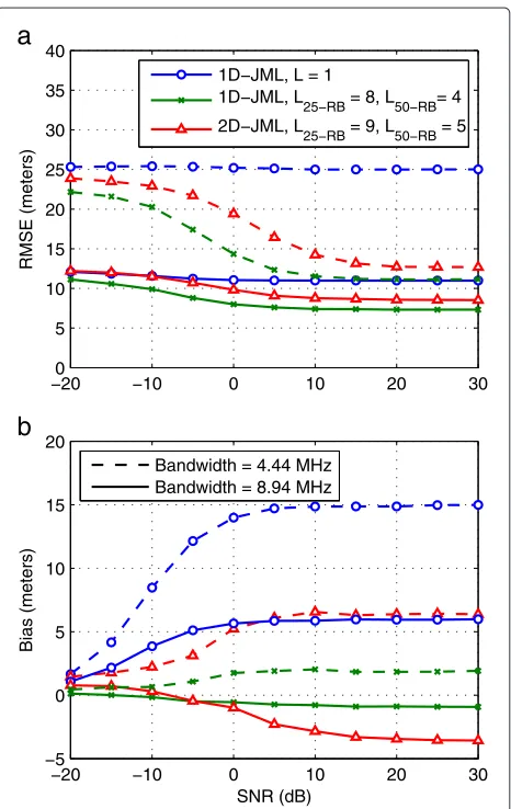
Considering the process followed in the previous section, the impact of multipath and noise is assessed for the typical signal bandwidths. The RMSE and the bias of
the 1D- and 2D-JML estimators for L > 1 outperform
the 1D-JML estimator forL = 1, as shown in Figure 10. Indeed, it is essential to use L > 1 with 25-RB band-width in order to obtain a satisfactory performance. As it can be seen in the figure, the 1D-JML estimator for
L > 1 achieves a slightly lower RMSE than the 2D-JML
0 1 2 3 4 5 6 7 8 0
0.2 0.4 0.6 0.8 1
b
a
Tap delay (Ts units)
Average power−delay profile
Signal bandwidth = 1/Ts = 4.44 MHz
0 1 2 3 4 5 6 7 8 9 10 11 12 13 14 15 16 17 0
0.2 0.4 0.6 0.8 1
Tap delay (Ts units)
Signal bandwidth = 1/Ts = 8.94 MHz
Average PDP Multipath delays
0 0.1 0.2 0.3 0.4 0.5 0
0.2 0.4 0.6 0.8 1
b
a
Absolute time delay error (Ts units)
CDF
Signal bandwidth = 1/Ts = 4.44 MHz
1D−JML, L = 1 1D−JML, L = 8 2D−JML, L = 9
0 0.1 0.2 0.3 0.4 0.5 0
0.2 0.4 0.6 0.8 1
Absolute time delay error (Ts units)
Signal bandwidth = 1/Ts = 8.94 MHz
1D−JML, L = 1 1D−JML, L = 4 2D−JML, L = 5
Figure 9CDF of the 1D- and 2D-JML time-delay estimations using ETU model without noise.(a)25-RB PRS bandwidth.(b)50-RB PRS bandwidth. One thousand channel realizations are used.
−200 −10 0 10 20 30
5 10 15 20 25 30 35 40
a
b
RMSE (meters)
−20 −10 0 10 20 30
−5 0 5 10 15 20
SNR (dB)
Bias (meters)
1D−JML, L = 1 1D−JML, L
25−RB = 8, L50−RB= 4
2D−JML, L
25−RB = 9, L50−RB = 5
Bandwidth = 4.44 MHz Bandwidth = 8.94 MHz
Figure 10Performance of 1D- and 2D-JML estimators using ETU model with AWGN and {25,50}-RB PRS bandwidth.(a) Root-mean-square error of the time-delay estimations.(b)Bias of the time-delay estimations. One thousand ETU model realizations per SNR are used.
estimator forL > 1 in both bandwidth cases. However, this difference between the 1D- and 2D-JML estimators
for L > 1 on the RMSE is as low as within 2 m for
both bandwidths. Considering the 50-RB PRS bandwidth (i.e. 8.94 MHz), the bias of both 1D-JML estimator for
L = 4 and 2D-JML estimator for L = 5 is below 5 m.
Thus, the JML estimation using the periodic-tap model and the novel hybrid-tap model exploits the LTE perfor-mance with a notable improvement with respect to the JML estimation using the single-tap model (i.e. matched filter or correlator), achieving a promising accuracy in usual working conditions.
6 Conclusions
smaller time-delay estimation errors than the matched filter, achieving a bias below 5 m.
Competing interests
The authors declare that they have no competing interests.
Acknowledgements
This work was supported by the ESA under the PRESTIGE programme ESA-P-2010-TEC-ETN-01 and by the Spanish Ministry of Economy and Competitiveness project TEC2011-28219.
Disclosure
The content of the present article reflects solely the authors view and by no means represents the official ESA view.
Author details
1Department of Telecommunications and Systems Engineering, Universitat Autònoma de Barcelona (UAB), Q Building, Cerdanyola del Vallès 08193, Spain. 2ESTEC, European Space Agency, Keplerlaan 1, 2200 AG, Noordwijk ZH, The Netherlands.
Received: 31 May 2013 Accepted: 28 February 2014 Published: 14 March 2014
References
1. 3GPP, LTE, Evolved Universal Terrestrial Radio Access (E-UTRA); physical channels and modulation (3GPP TS 36.211, version 9.1.0 Release 9), Technical specification
2. 3GPP, LTE, Evolved Universal Terrestrial Radio Access Network (E-UTRAN); stage 2 functional specification of user equipment (UE) positioning in E-UTRAN (3GPP TS 36.305, version 9.10.0 Release 9), Technical specification 3. J Medbo, I Siomina, A Kangas, J Furuskog, Propagation channel impact on
LTE positioning accuracy: a study based on real measurements of observed time difference of arrival, inProceedings of IEEE 20th International Symposium on Personal, Indoor and Mobile Radio Communications (PIMRC)
(Tokyo, 13–16 September 2009), pp. 2213–2217
4. C Gentner, E Muñoz, M Khider, E Staudinger, S Sand, A Dammann, Particle filter based positioning with 3GPP-LTE in indoor environments, in
Proceedings of the IEEE/ION Position Location and Navigation Symposium (PLANS)(Myrtle Beach, 23–26 April 2012), pp. 301–308
5. JA del Peral-Rosado, JA López-Salcedo, G Seco-Granados, F Zanier, M Crisci, Analysis of positioning capabilities of 3GPP LTE, inProceedings of the 25th International Technical Meeting of the Satellite Division of the Institute of Navigation (ION GNSS)(Nashville, 17–21 September 2012), pp. 650–659 6. 3GPP, LTE, Evolved Universal Terrestrial Radio Access (E-UTRA); user
equipment (UE) radio transmission and reception (3GPP TS 36.101, version 9.18.0 Release 9), Technical specification
7. 3GPP, LTE, Evolved Universal Terrestrial Radio Access (E-UTRA); base station (BS) radio transmission and reception (3GPP TS 36.104, version 9.13.0 Release 9), Technical specification
8. B Yang, KB Letaief, RS Cheng, Z Cao, Timing recovery for OFDM transmission. IEEE J. Selected Areas Commun.18(11), 2278–2291 (2000) 9. J Vidal, M Nájar, R Játiva, High resolution time-of-arrival detection for
wireless positioning systems, inProceedings of the IEEE 56th Vehicular Technology Conference (VTC), vol. 4 (Vancouver, 24–28 September 2002), pp. 2283–2287
10. X Li, K Pahlavan, Super-resolution TOA estimation with diversity for indoor geolocation. IEEE Trans. Wireless Commun.3(1), 224–234 (2004) 11. O Bialer, D Raphaeli, AJ Weiss, Efficient time of arrival estimation algorithm
achieving maximum likelihood performance in dense multipath. IEEE Trans. Signal Process.60(3), 1241–1252 (2012)
12. K Schmeink, R Adam, PA Hoeher, Performance limits of channel parameter estimation for joint communication and positioning. EURASIP J. Adv. Signal Process.2012(178), 1–18 (2012)
13. WU Bajwa, J Haupt, G Raz, R Nowak, Compressed channel sensing, in
Proceedings of the 42nd Annual Conference on Information Sciences and Systems (CISS)(Princeton, 19–21 March 2008), pp. 5–10
14. K Gedalyahu, YC Eldar, Time-delay estimation from low-rate samples: a union of subspaces approach. IEEE Trans. Signal Process.58(6), 3017–3031 (2010)
15. J Yang, X Wang, SI Park, HM Kim, Direct path detection using multipath interference cancellation for communication-based positioning system. EURASIP J. Adv. Signal Process.2012(188), 1–18 (2012)
16. EG Larsson, G Liu, J Li, GB Giannakis, Joint symbol timing and channel estimation for OFDM based WLANs. IEEE Commun. Lett.5(8), 325–327 (2001)
17. M-O Pun, M Morelli, C-CJ Kuo, Maximum-likelihood synchronization and channel estimation for OFDMA uplink transmissions. IEEE Trans. Commun.54(4), 726–736 (2006)
18. L Sanguinetti, M Morelli, An initial ranging scheme for IEEE 802.16 based OFDMA systems, inProceedings of the 8th International Workshop on Multi-Carrier Systems & Solutions (MC-SS)(Herrsching, 3–4 May 2011), pp. 1–5
19. H Zhou, Y-F Huang, A maximum likelihood fine timing estimation for wireless OFDM systems. IEEE Trans. Broadcasting55(1), 31–41 (2009) 20. MD Larsen, G Seco-Granados, AL Swindlehurst, Pilot optimization for time-delay and channel estimation in OFDM systems, inProceedings of the IEEE International Conference on Acoustics, Speech and Signal Processing (ICASSP)(Prague, 22–27 May 2011), pp. 3564–3567
21. JA López-Salcedo, E Gutiérrez, G Seco-Granados, AL Swindlehurst, Unified framework for the synchronization of flexible multicarrier communication signals. IEEE Trans. Signal Process.61(4), 828–842 (2013)
22. JA del Peral-Rosado, JA López-Salcedo, G Seco-Granados, F Zanier, M Crisci, Joint channel and time-delay estimation for LTE positioning reference signals, inProceedings of the 6th ESA Workshop on Satellite Navigation User Equipment Technologies (NAVITEC)(Noordwijk, 5–7 December 2012), pp. 1–8
23. J Proakis,Digital Communications, 4th edn (McGraw-Hill, New York, 2000) 24. T Yücek, H Arslan, Time dispersion and delay spread estimation for
adaptive OFDM systems. IEEE Trans. Vehicular Technol.57(3), 1715–1722 (2008)
25. GH Golub, V Pereyra, The differentiation of pseudo-inverses and nonlinear least squares problems whose variables separate. SIAM J. Numerical Anal.
10(2), 413–432 (1973)
doi:10.1186/1687-6180-2014-33
Cite this article as:del Peral-Rosadoet al.:Joint maximum likelihood time-delay estimation for LTE positioning in multipath channels.EURASIP Journal on Advances in Signal Processing20142014:33.
Submit your manuscript to a
journal and benefi t from:
7Convenient online submission 7Rigorous peer review
7Immediate publication on acceptance 7Open access: articles freely available online 7High visibility within the fi eld
7Retaining the copyright to your article