Hierarchical Classification of Liver Tumor from CT Images Based on Difference-of-features (DOF)

Hierarchical Classification of Liver Tumor from CT

Images Based on Difference-of-features (DOF)

Hussein Alahmer, Amr Ahmed

Abstract—This manuscript presents an automated classification approach to classify lesions into four categories of liver diseases, based on Computer Tomography (CT) images. The four diseases types are Cyst, Hemangioma, Hepatocellular carcinoma (HCC), and Metastasis.

The novelty of the proposed approach is attributed to utilizing the difference of features (DOF) between the lesion area and the surrounding normal liver tissue. The DOF (texture and intensity) is used as the new feature vector that feeds the classifier. The classification system consists of two phases. The first phase differentiates between Benign and Malignant lesions, using a Support Vector Machine (SVM) classifier. The second phase further classifies the Benign into Hemangioma or Cyst and the Malignant into Metastasis or HCC, using a Naïve Bayes (NB) classifier. The experimental results show promising improvements to classify the liver lesion diseases. Furthermore, the proposed approach can overcome the problems of varying intensity ranges, textures between patients, demographics, and imaging devices and settings.

Keywords—CAD system, Difference of feature, Fuzzy-c- means, Lesion detection, Liver segmentation.

I. INTRODUCTION

iver is an important organ to human where it performs vital functions such as detoxification of hormones, drugs, filter the blood from waste products, production of proteins required for blood clotting. Therefore, liver disease has to be considered seriously. The early detection and correct diagnose will-assist to reduce the cancer death and will lead to a successful treatment and full recovery. There are two classes of a liver lesion: benign and malignant. The benign lesions (noncancerous) are quite common and usually do not produce symptoms. For this work Hemangioma, and Cyst considered as benign. Malignant lesions (cancerous) are divided into primary liver cancer where originated in the liver and metastatic liver cancer which spreads from cancer sites elsewhere in the body. Metastasis and HCC considered as malignant [1].

There are several types of imaging techniques performed for examination of liver tumors such as Computed tomography (CT) scan, Ultrasound, X-Ray, and Magnetic Resonance Imaging (MRI) to diagnose liver tumors. The CT scan considers one of the most robust imaging modalities. Although during the last years, the quality of CT images has been significantly improved. Moreover, a vast amount of information can be obtained from CT [2].

Manuscript received March 17, 2016; revised March 29, 2016. Hussein Alahmer, is a PhD researcher at School of Computer Science, University of Lincoln, Brayford Pool, Lincoln, LN6 7TS (e-mail: [email protected]).

Amr Ahmed is a Faculty Members of School of Computer Science, University of Lincoln, Brayford Pool, Lincoln, LN6 7TS (e-mails: [email protected]).

However, experienced doctors face some difficulties to make an accurate diagnosis that leads to more tests and invasive procedures (biopsies) [3]. Computer-aided diagnosis (CAD) systems were proposed for liver tissue characterization and classification, and gained more attention within the evolution in image processing and artificial intelligence to adopt as a second hand for the radiologist and assist in diagnosis and reduce the number of biopsy or surgery that would otherwise have been necessary [4].

The CAD system considers feature extraction as important stage, which is used in lesion classification and applied for understanding radiological images by extracting low level features such as intensity, texture, and shape features and feed them to a classifier to diagnose liver tumors [5], [6]. Therefore, several approaches have been applied to determine the appropriate features to fuel classifiers in order to increase the diagnostic accuracy.

In this paper, an overview of various liver diseases’ classification methodologies is explained briefly. The novelty of this work lies in using the difference of intensity and texture features between a lesion and its surrounding area from normal liver tissue. The classification is done through two phases. Firstly, proposed system classified lesion into benign or malignant. Secondly, reclassify benign into Hemangioma or Cyst and malignant into Metastasis or HCC.

The paper is organised as follows. Section II presents the related literature research, section III presents the proposed work, which includes Liver segmentation and lesion detection, feature extraction, and classification; section IV deals with the experiments results and discussion while section V summarizes the study findings through the conclusion.

II.RELATED WORK

Numerous CAD systems have been developed to classify the liver tumors into benign and malignant. While other systems proposed to classify specific liver diseases such as Cyst, Hemangioma, Hepatic adenoma and Focal nodular hyperplasia (which are of benign); Metastatic, HCC, and Cholangiocarcinoma (which are malignant).

Extracting appropriate features is considered to be the most important stage in CAD system for classification of liver diseases. Hence, previous research developed the accuracy of the CAD system to classify the liver lesion based on a type of features. These features can be categorised depending on the type of features, into intensity-based features, texture-intensity-based features or combined features between intensity and texture to be fed to a classifier.

Dankerl et al. [7] proposed a CAD system where uses an image search engine exploiting texture analysis of liver

tumor image data for enquiry tumors from a database to retrieve the lesion type (Cyst, Hemangioma, HCC, and Metastasis). The radiologist has drawn ROI around the lesion. Total number of images is 80 that used for training and testing, which divided into 20 Hemangioma, 20 Metastasis, 20 HCC, and 20 Cysts and it recorded an accuracy rate 95.5%.

In yet another classification of liver tissue from CT images system was presented by Mougiakakou et al. [8]. The lesions were drawn by an experienced radiologist as a region of interest corresponding to the normal liver tissue, Cyst, Haemangioma, and HCC. Five different types of texture features are extracted for each ROI as the following, first-order statistics, spatial gray level dependence matrix, gray level difference method, Laws texture energy measures, and fractal dimension measurements. The dataset size 147; 83 have been used as training set, 32 as validation set, and 32 as testing. However, the majority of the cases in the dataset are normal liver tissue as 76 samples. CAD system depends on multiple classifier system consist from five Neural Networks (NNs), a system used one of NN as primary classifier and other four NNs trained by back-propagation algorithm with adaptive learning rate and momentum. Final classification results are based on the application of a voting scheme across the outputs of the individual NNs with obtained 90.63% accuracy for testing set and 93.75% for the validation set.

Additional study in liver classification was provided by Safdari et al. [9]. The classification system was developed to characterize the liver lesion in CT image into Haemangioma, Metastasis, and Cyst based using a visual word histogram. While the proposed system builds a dictionary for a training set using local descriptors and representing a region in the image using a visual word histogram. Where, a scan window moves across the image and is determined to be normal liver tissue or a lesion. The radiologist determined the liver boundary and drew ROI around the lesion. Totally dataset 73 cases divided into 25 Cysts, 24 Metastases, and 24 Haemangiomas. The accuracy recorded was 95%.

The most recently study in liver lesion classification was provided by Doron et al. [10]. The combination of texture features (GLCM, LBP, Gabor, and GLBP) and intensity feature (gray level intensity) are obtained from a given lesion. For classification module, SVM and KNN classifier were used to distinguish between four types of liver tissues, namely: Cyst, Hemangioma, Metastases, and Healthy tissue. The best result of 97% accuracy was obtained with combination of Gabor, LBP and Intensity features using SVM classifier.

Table I depicts a generic comparison between various proposed CAD systems as previously stated.

After surveying the published papers, many researchers try to diagnose liver disease using different techniques to increase the classification performance. However, it has been found that the previous studies on CAD systems usually used the absolute value of features, which are extracted from lesion regions. As a consequence, the performance is varied significantly under different acquisition conditions. For example, the CT machines or operators are different. In this study the surrounding normal

tissue of liver in the same image is used as reference. So for a certain feature, we calculate the difference of features between the lesion and surrounding normal liver tissue and employ it as a new feature vector in our proposed system.

TABLE I

OVERVIEW OF DISCUSSED CAD SYSTEM

Da

tas

et

size

H

CC

C

y

st

H

a

ema

ng

io

ma

M

etas

tas

is

Accuracy

Dankerl et al. [7] 80 x x x x 95.5%

Mougiakakou et al. [8] 147 x x x - 93.75%

Safdari et al. [9] 73 - x x x 95%

Doron et al. [10] 92 x x x x 97.3%

III.PROPOSED WORK

The main goal of this paper is to design a CAD system to classify CT liver lesion at the first stage into one of the two classes: benign and malignant as presented in figure 1. Then, reclassified as disease type into Hemangioma or Cyst for benign and Metastasis or HCC for malignant.

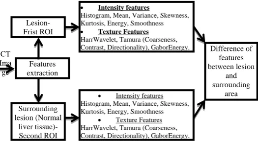
Firstly, Regions of Interest (ROIs) that reflect lesion is being detected automatically by the proposed system from CT images. Secondly, the area surrounding the lesions from the normal liver tissue are extracted by the proposed system is driven to a feature extraction module, where three different texture feature sets are obtained using HarrWavelet, Tamura (Coarseness, Contrast, Directionality) and GaborEnergy, and seven intensity features are calculating through Histogram, Mean, Variance, Skewness, Kurtosis, Energy and Smoothness. In addition to a five shape features. Namely, area, dispersion, elongation, and two circularity of lesion features. Then, the shape features and combined difference between the features value (texture and intensity) from the lesion and the surrounding normal liver tissue were fed into SVM in the first phase to classify lesions either benign or malignant. Naïve Bayes classifier is used in a second phase to classify the output from phase one into possible one of the four types of disease, Hemangioma, Cyst, HCC, and Metastasis.

 CAD system

Fig. 1. CAD system architecture

A. Liver and lesion segmentation

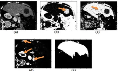
The system uses two-step processes. Firstly, segment the liver by generating the binary liver mask. The CT grayscale image is split into three classes using a memory efficient implementation of the fuzzy c-means (FCM) clustering algorithm [11], [12] as illustrated in figure 2.

Fig. 2. Liver and Lesion detection: (a) Original CT image; (b) Lesion highlighted; (c) Liver highlighted; (d) Other organs highlighted; (e) Liver mask.

The computational efficiency is achieved by using the histogram of the image intensities during the clustering process instead of the raw image data. After that the combinations of several morphological operations were applied to remove the small object outside the liver region where the liver defined as the largest connected pixel. The morphological operation is defined as follows:

𝑓 ∗ 𝑏 = (𝑓 𝑏)০𝑏 (1)

Where fis the target image, b is the structuring element, () means morphological closing, and ০ means morphological opening . Then region growing is applied to segment tumors [13], where the region is iteratively grown by comparing all unallocated neighbouring pixels to the region. The difference between a pixel intensity value and the region mean is used as a measure of similarity. The pixel with the smallest difference measured this way is allocated to the respective region. This process stops when the intensity difference between region mean and new pixel become larger than a certain threshold (t). The optimum threshold was calculated based on measures of fuzziness to detect the ambiguous pixels, such that pixels with membership values greater than or equal to the threshold will be assigned to the appropriate clusters and those pixels with membership values less than the threshold will be marked as ambiguous cluster. The process of liver and lesion segmentation from CT image is presented in figure 3.

Fig. 3. Liver and Lesion segmentation process: (a) Histogram for CT; (B) Original CT image; (C) Extracted liver with noise; (d) After morphological operation; (e) Detected lesion; (f) Segmented lesion.

After extracting the liver and defined the lesion, the proposed system will be cropped the lesion and normal liver tissue that surrounding lesion where excluded the lesion area to extract the features from both ROI.

B. Feature Extraction

The next stage in our proposed system is feature extraction, which is considered a critical step in the CAD system to classify/characterise the lesion. Basically there is a large diverse set of features to be used. Those come under three categories; intensity, shape, and texture feature.

First of all, the proposed system defines two types of ROI for extracting the features relating to intensity and texture. The first ROI is the lesion, and the second ROI is the surrounding normal liver tissue as shown in figure 4. The difference of features value between normal and lesion were used in classification.

In contrast with current trends about identification of lesions using one ROI (lesion area only), we proposed to use a second ROI which surrounds the first ROI. Moreover, the second ROI will be used as well to extract features. The difference of features between the first ROI and the second ROI will be employed as a new feature vector. But there are some constrains to identify the second ROI: (1) The second ROI must be centrally surrounding the first ROI. (2) The ratio between the first and second ROIs are 1:1.5, reached by doing several attempts. (3) The first ROI is excluded from the second ROI region. As displayed in figure 4. (d).

Fig. 4. Lesion and normal liver tissue segmentation: (a) Original CT image; (b) First ROI is red box for lesion and second ROI is blue box for surrounding normal liver tissue; (c) cropped lesion box; (d) cropped surrounding normal liver tissue box.

Test Data

Building Classification

Model Training

Data Classification

Processing (Crop lesion and surrounding

area)

Difference-features Measurements

Classification Phase 1- B/M

Phase 2- Disease type

Processing (Crop lesion and

surrounding area)

Difference-features Measurements

Model CT

Ima ge

Features extraction Lesion- Frist ROI

Surrounding lesion (Normal

liver tissue)- Second ROI

 Intensity features

Histogram, Mean, Variance, Skewness, Kurtosis, Energy, Smoothness

 Texture Features HarrWavelet, Tamura (Coarseness,

Contrast, Directionality), GaborEnergy. _{Difference of}

features between lesion

and surrounding

area  Intensity features

Histogram, Mean, Variance, Skewness, Kurtosis, Energy, Smoothness

 Texture Features HarrWavelet, Tamura (Coarseness, Contrast, Directionality), GaborEnergy.

Fig. 5. Features extraction process

The intensity features derived from histogram features, which describe the relative frequency of pixel intensity value in the image which consider Mean, Standard Deviation, Skewness, Kurtosis [16]–[18]. The mean (µ) calculates the estimation of the average level of intensity in the ROI region.

µ =1

𝑁 (𝑥,𝑦)∈𝑅𝑂𝐼𝐼(𝑥, 𝑦)

(2) Where, I(x,y) is the gray level at pixel (x,y), and I is the total number of pixel inside the ROI. The difference of mean gray level between the lesion and surrounding normal liver tissue is:

𝑑𝑖𝑓𝑓𝑒𝑟𝑒𝑛𝑐𝑒 𝜇 =1

𝑁 𝑥,𝑦 ∈𝑅𝑂𝐼𝐼𝑁𝑜𝑟𝑚𝑎𝑙 𝑥, 𝑦 − 1

𝑀 (𝑥,𝑦)∈𝑅𝑂𝐼𝐼𝑙𝑒𝑠𝑖𝑜𝑛 (𝑥, 𝑦) (3) where INormal(x,y) means the gray level at pixel (x,y) of normal surrounding liver tissue ROI, ILesion(x,y)means the gray level at pixel (x,y) of lesion ROI, M is the total number of pixels inside the ROI of normal liver and N is the total number of pixels inside the ROI of lesion.

Standard deviation (σ) is a measure of the dispersion of intensity

σ = 1

𝑁 (𝑥𝑖− μ) 2 𝑁

𝑖=1 (4)

Skewness (γ₁) is a measure of histogram symmetry

γ1= 1

𝑁∗𝜎3 𝑁𝑖=1(𝑥𝑖− μ)3 (5) Kurtosis (K) is a measure of the tail of the histogram.

𝐾 = 1

N∗𝜎4 (𝑥𝑖− μ)4

𝑁

𝑖=1 (6) Where the difference of Standard deviation, Skewness, and kurtosis between normal liver tissue and lesion is calculated in the same way as mentioned previously in the mean calculation.

As well as, three types of texture features (HaarWavelet, Gabor energy, and Tamura (Coarseness, Contrast, and Directionality)) were extracted for each ROI. Gabor feature used to measure the similarities between Gabor mask and neighbourhoods in the image. Each Gabor mask consists of Gaussian windowed sinusoidal waveforms. While Tamura’s feature extracted to calculate coarseness, contrast, and directionality. The difference of features was used to replace the lesion features absolute value.

For each lesion ROI, the feature extraction module calculates a five shape feature. Namely, area, dispersion, elongation, and two circularity of lesion features.

Area of the segmented lesion is computed by counting the number of pixels inside the ROI1.

𝐴 = 𝑛[ROI₁] (7)

Where, n[ROI₁] represents the count of number of the pixel inside lesion.

Dispersion property is estimating the irregularity of the lesion, which identifies the irregular shape by the equation below.

Dispersion =𝑀𝑎𝑥 𝑅𝑎𝑑𝑖𝑢𝑠

𝐴𝑟𝑒𝑎 (8) Elongation property is differentiating the regular oval mass from the irregular. This value is given by the following equation.

Elongation = 𝐴𝑟𝑒𝑎

(2∗𝑀𝑎𝑥 𝑅𝑎𝑑𝑖𝑢𝑠 )2 (9)

The circularity of the lesion is expressed by the following equation. Where the result takes a value of 1 for perfect circles.

circularity 1 = _{(𝜋∗ 𝑀𝑎𝑥 𝑅𝑎𝑑𝑖𝑢𝑠}𝐴𝑟𝑒𝑎 2₎ (10)

Moreover, the following formula is useful in differentiating circular/ oval lesion from irregular. Where the result takes a value of 1 for perfect circles. This value measures how a lesion is similar to an ellipse.

circularity 2 = 𝑀𝑖𝑛 𝑅𝑎𝑑𝑖𝑢𝑠

𝑀𝑎𝑥 𝑅𝑎𝑑𝑖𝑢𝑠 (11)

C. Classification

Classification is the last stage in an automated CAD system, where its input is the extracted set of feature vectors(s) from the previous stage. The goal of the classification stage is to apply a learning-based approach considering its input feature vector(s), for the purpose of disease diagnosis.

After extraction the features from liver lesion and normal liver tissues that surrounding the lesion then the difference between them is computed and used as an input to the 2-phase classifier. Phase-1 uses Support Vector Machine (SVM) to classify lesion as benign or malignant and phase-2 uses Naïve Bayes (NB) to classify types of liver disease.

IV.EXPERIMENTAL RESULTS

This section contains the experimental model. The dataset (presented later) divided into testing data and training data. The experiment focused on extract the features from both of lesion and normal liver tissue that surround the lesion then use the difference between of them to build a feature vector. A new feature vector used to feed the classifier to differentiate between liver lesion into benign or malignant for the first phase and then reclassify as a type of disease in the second phase. As shown in figure 6.

A. Dataset and experimental setup

We obtained 60 patient cases, where liver lesions are identified in CT scan and divided into malignant (18 Metastases, 15 HCC) and benign (14 Cysts, 13 Hemangioma) for training. The CT images had varied resolutions (x: 190-308 pixels, y: 213-387 pixels, slices: 41-588) and spacing (x, y: 0.674-1.007mm, slice: 0.399-2.5mm).

The experiments have been done on Intel Core I5- 3.40 GHz computer with 8 Gigabytes of RAM under windows 7 64-bit operating system. The Matlab R2014a was used to run experiments and extract the features and Weka 3.6.11 machine learning tool [21] was used for classification.

B. Evaluation and result

This section will be displayed the evaluation and result for each segmentation stage and classification lesion in our proposed system.

 Segmentation phase

The proposed system was tested on whole dataset. To measure the segmentation performance in all cases the two coefficients are used to obtain the accuracy of the liver segmentation, namely: Jaccard similarity metric (JC), also known as the Tanimoto coefficient [14], and Dice coefficient [15].

Fig. 7. evaluation of Liver segmentation: (a) Ground truth of Liver segmentation by radiologist; (b) Overlap liver segmentation proposed system and ground truth; (c) Box is ground truth of the lesion drawn by expert and red area is the mask generated by proposed system; (d) Set matching indicated are the true negative, false positive, false negative, and true positive areas.

As shown in figure 7, we define X as a set of all pixels in the image. The ground truth T ∈ X as the set of pixels that were labelled as liver by the radiologist. Similarly, we defined S ∈ X as the set of pixels that were labelled as liver by the proposed system.

A true positive set is defined as TP = T ∩ S, the set of pixels common to T and S. True negative is define as TN = T

∩ S , the set of pixels that were labelled as non-liver in both sets. Similarly, the false positive set is FP = T ∩ S and the false negative set is FN = T ∩ S .

Jaccard similarity metric, 𝐽 𝑇, 𝑆 = 𝑇∩𝑆 _𝑇∪𝑆 = _{𝑇𝑃 + 𝐹𝑃 + 𝐹𝑁} 𝑇𝑃 (12)

Dice coefficient, 𝐷 𝑇, 𝑆 =2∗ 𝑇∩𝑆 _{𝑇 + 𝑆} = _{𝑇𝑃 + 𝐹𝑁 + 𝑇𝑃 + 𝐹𝑃} 2 ∗ 𝑇𝑃 (13) The evaluate accuracy of the proposed liver segmentation method compared to the ground truth; we utilise Jaccard and Dice coefficient method which depicted in the equation 7 and 8. The accuracy of segmentation was 0.82 and 0.9 respectively.

 Classification phase

The proposed system was tested on a CT image dataset through used 12 pathological CT sets, divided into malignant (3 Metastases, 3 HCC) and benign (3 Cysts, 3 Hemangioma). The classifier output compared with original class attribute to generate confusion matrix and identifying True Positive (TP) were malignant disease classified as malignant disease correctly, True Negative (TN) benign disease classified as benign disease correctly, False Positive (FP) classified benign disease incorrectly as malignant disease, and False Negative (FN) classified malignant disease incorrectly as benign disease.

To evaluate the proposed classification performance several standard measures were used, as defined as below:

Accuracy= (TP+TN)/ (TP+TN+FP+FN) (14) Sensitivity=TP/ (TP+FN) (15) Specificity=TN/ (TN+FP) (16)

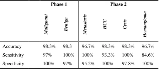
The result of the experiments is presented in table II. It shows that higher accuracy classification result is achieved when divided classification into two stages and using the novelty feature difference between normal liver tissue around the lesion and the lesion to record 97.5% comparing with other experiments without divided into two phases, and the accuracy obtained 94.17%. As The ROC curve is presented in figure 10.

Fig. 10. ROC curve of accuracy for the diagnosis of four types of lesion, using a two phases for classification and direct classification.

TABLE II

RESULT OF THE EXPERIMENT FOR BOTH PHASES (DIFFERENCE OF FEATURES TECHNIQUE WERE USED)

Phase 1 Phase 2

Ma

li

g

n

a

n

t

B

en

ign

M

etastasi

s

HCC Cys

ts

H

emangi

o

m

a

Accuracy 98.3% 98.3 96.7% 98.3% 98.3% 96.7%

Sensitivity 97% 100% 100% 93.3% 100% 84.6%

Specificity 100% 97% 95.2% 100% 97.8% 100%

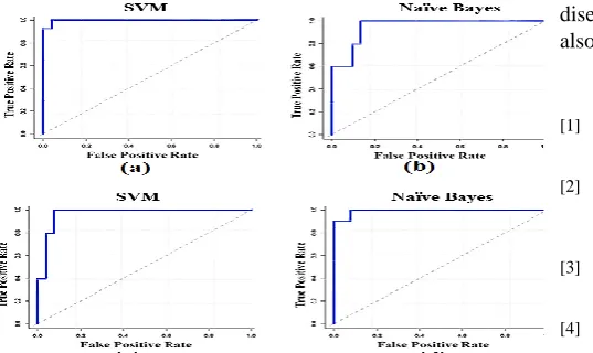
The proposed system used two type of classifier SVM and Naïve Bayes. SVM adopted to classify liver lesion into benign and malignant. Naïve Bayes used to reclassify benign into Cyst and Hemangioma, Malignant into Metastasis and HCC, where used accuracy, sensitivity and specificity to measure the performance of the proposed system as mentioned in table II.

Fig. 11. ROC curve for SVM and NB: (a) ROC curve SVM in phase one; (b) ROC curve NB in phase one; (c) ROC curve SVM in phase two; (d) ROC curve NB in phase two.

The baseline Doron et al [10] is already introduced in detail in literature section. This baseline is selected since it’s the most recent baseline. Moreover, it represents the state-of-art with its high accuracy. Due to the limited availability of the used dataset, we have regenerated the baseline by implementing [10] and applying it on our dataset. The result of the proposed system compared, to the baseline, is shown in Table III.

TABLE III

COMPARISON BETWEEN PROPOSED METHODS AND BASELINE

Malignant/Benign

M

etas

tas

is

H

CC

C

y

sts

H

ema

ng

io

ma

Baseline 91.7% 93.2% 91.5% 94.9% 93.2%

Proposed 98.3% 96.7% 98.3% 98.3% 96.7%

The importance of the proposed system is the ability to classify the liver lesion into benign and malignant with the high accuracy 98.3% through the novelty of building feature vector based on the difference of feature between a lesion and normal liver tissue that surround the lesion and reclassify benign and malignant into a specific type of liver disease (HCC, Cyst, Hemangioma, and Metastasis) to record the average accuracy 97.5%.

V.CONCLUSION

This paper proposed a two phases approach to classify liver diseases, depending on a feature-difference approach, from CT scan images. In the first phase, it classifies a lesion into benign or malignant. Then, in the second phase, it further classifies the lesion into Cysts, Hemangioma, Metastasis, or HCC. The novelty of the proposed approach is the use of difference-of-features (DOF) from the lesion and the surrounding normal tissues. Also, the hierarchical classification approach helps in improving the classification further into the four diseases. This DOF has improved the accuracy to 98.3% for benign and malignant in the first phase, and to 97.5% for Cysts, Hemangioma, HCC and Metastasis in the second phase. More importantly, the DOF helps overcoming one of the major issues, namely the variation of intensity and texture ranges between different patients, ages, demographics and/or imaging devices. The proposed system can be extended for other types of liver

diseases such as cholangiocarcinoma, and abscesses and also for other types of medical images like MRI.

REFERENCES

[1] A. Jemal, F. Bray, Center, M. Melissa, J. Ferlay, E. Ward, and D. Forman, CA: A Cancer Journal for Clinicians. 61: 69–90. doi: 10.3322/caac.20107, 2011.

[2] M. Arne, T. Hager, F. Jager, C. Tietjen, and J. Hornegger. "Automatic detection and segmentation of focal liver lesions in contrast enhanced CT images." In Pattern Recognition (ICPR), 2010 20th International Conference on, pp. 2524-2527. IEEE, 2010

[3] I. Sporea, A. Popescu, and R. Sirli. Why, who and how should perform liver biopsy in chronic liver diseases. World journal of gastroenterology: WJG, 14(21): 3396, 2008.

[4] P. Dankerl, A. Cavallaro, M. Uder, and M. Hammon. Automatisierte Segmentierung und Annotation in der Radiologie. Der Radiologe, 54(3): 265-270, 2014.

[5] A. Depeursinge, C. Kurtz, C. Beaulieu, S. Napel, D. Rubin, “Predicting Visual Semantic Descriptive Terms From Radiological Image Data: Preliminary Results With Liver Lesions in CT," Medical Imaging, IEEE Transactions on, 33(8): 1669-1676, 2014.

[6] P. Taylor, " A review of research into the development of radiologic expertise: Implications for computer-based training." Academic radiology, 14(10): 1252-1263, 2007.

[7] P. Dankerl, A. Cavallaro, A. Tsymbal, J. Costa, M. Suehling, R. Janka, and M. Hammon,. "A retrieval-based computer-aided diagnosis system for the characterization of liver lesions in CT scans".

Academic radiology, 20(12): 1526-1534, 2013.

[8] S. Mougiakakou, I. Valavanis, K. Nikita, A. Nikita, and D. Kelekis. "Characterization of CT liver lesions based on texture features and a multiple neural network classification scheme." In Engineering in Medicine and Biology Society, 2013. Proceedings of the 25th Annual International Conference of the IEEE, vol. 2: 1287-1290. IEEE, 2013. [9] M. Safdari, R. Pasari, D. Rubin, and H. Greenspan. "Image

patch-based method for automated classification and detection of focal liver lesions on CT". In SPIE Medical Imaging (pp. 86700Y-86700Y). International Society for Optics and Photonics. 2013.

[10] Y. Doron, N. Mayer-Wolf, I. Diamant, and H. Greenspan. "Texture feature based liver lesion classification." In SPIE Medical Imaging, pp. 90353K-90353K. International Society for Optics and Photonics, 2014.

[11] Wu, Kuo-Lung, and Miin-Shen Yang. "Alternative c-means clustering algorithms." Pattern recognition, 35(10): 2267-2278, 2002.

[12] Yang, Miin-Shen, Yu-Jen Hu, Karen Ren Lin, and Charles Chia-Lee Lin. "Segmentation techniques for tissue differentiation in MRI of ophthalmology using fuzzy clustering algorithms." Magnetic Resonance Imaging, 20(2): 173-179, 2002.

[13] Zhao, Binsheng, Lawrence H. Schwartz, Li Jiang, Jane Colville, Chaya Moskowitz, Liang Wang, Robert Leftowitz, Fan Liu, and John Kalaigian. "Shape-constraint region growing for delineation of hepatic metastases on contrast-enhanced computed tomograph scans."

Investigative radiology, 41(10): 753-762, 2006.

[14] P. Jaccard, "The distribution of the flora in the alpine zone. 1." New phytologist, 11(2): 37-50, 1912.

[15] L. Dice, "Measures of the amount of ecologic association between species." Ecology, 26(3): 297-302, 1945.

[16] K. Rodenacker, and E. Bengtsson. "A feature set for cytometry on digitized microscopic images." Analytical Cellular Pathology, 25(1): 1-36, 2003.

[17] CAO, Jian, Hai-sheng LI, Qiang CAI, and Shi-long Guo. "Research on Feature Extraction of Image Target." Computer Simulation, 30(1): 409-413, 2013.

[18] A. Chadha, M. Sushmit, and J. Ravdeep. "Comparative Study and Optimization of Feature-Extraction Techniques for Content based Image Retrieval." arXiv preprint arXiv:1208.6335, 2012.

[19] R. Entezari-Maleki, R. Arash, and B. Minaei-Bidgoli. "Comparison of classification methods based on the type of attributes and sample size." Journal of Convergence Information Technology 4.3: 94-102, 2009.

[20] J. Huang, L. Jingjing, and X. Charles. "Comparing naive Bayes, decision trees, and SVM with AUC and accuracy." In Data Mining, 2003. ICDM 2003. Third IEEE International Conference on, pp. 553-556. IEEE, 2003.