The ECL Optimization and Experiment of HSPMSM with Improved Method

Abstract — The eddy current loss should be optimized to be as less as possible for the stability of permanent magnet in high speed permanent magnet synchronous motor (HSPMSM) rotor and ensure the high efficiency and low temperature of the motor. This paper analyzes the eddy current distribution in rotor, with consideration of the conflict of the thickness of sleeve and diameter of the rotor, calculating the eddy current loss (ECL) and the thermal distribution via Separation of variables method for solving Maxwell's equations with analytical hieratical model of ECL constructed. The optimization result of ECL of the HSPMSM whose power and rated speed is 30kw 48000r/min can be got by multi-objective optimization method, combined weighting coefficient method and traversal algorithm based on chaotic local search particle swarm optimization (CLSPSO), utilizing ECL analytical model and other analytical constraints. Related experiment and measurement has been implemented with new approach of loss separation.

Index Terms—eddy current loss, multi-objective optimization (MOO), electromagnetic analysis, equivalent hierarchical method

I. INTRODUCTION

As for the HSPMSM, the ECL of rotor of which has higher speed occupies higher percentage of total loss especially in similar power level [1-4]. The component of ECL consists of spatial harmonic loss and time harmonic loss which occupies the mainly part when the HSPMSM reach more fast speed[5-7]. The higher ECL causes higher temperature rise and higher thermal stress, which threatens the operating stability of HSPMSM. The ECL in the rotor is usually appears significant when the PMSM operates at a higher speed [8].the harmonics ECL caused by space harmonics and time harmonics of flux density increase the temperature of rotor. This article mainly focus on

investigation of ECL mainly caused by harmonics in rotor and the reduction approach of it via optimization process.

With consideration of the PWM harmonics and the ECL caused by differential electromotive force, the main source of ECL is caused by harmonics [9-15]. Therefore, The ECL in rotor can be separated by each order harmonic ECL, which is asynchronous with the stator current, on which we based, the ECL analysis method of asynchronous motor can be used in PMSM, by which each order harmonic ECL can be calculated. During that computation process, the equivalent current sheet method can be utilized in equal to stator current density.

Since the ECL impacts the performance of the HSPMSM in every aspect, the optimization should be considered both in temperature rise and structural strength of rotor, as well as based on the ECL amount. The conventional multi-objective optimization mainly focused on weighted coefficient method [16-18], since its stable convergence, however, with the instability to arrive at the PARETO front ignored. Besides, the GA [19] and other evolution algorithms such as

Response Surface Methodology [20].et have been utilized in MOO with practical model involved [21-22]. The traversal algorithm runs lack of stability of convergence [23-24]. Thus, the combination of those two approaches can be utilized in MOO of HSPMSM via improved algorithm and adjusted parameters. The constraints are often transformed to penalty functions added to the objective function based on particle swarm optimization (PSO) [25-26] and harmony search (HS) [27] algorithm.et [28-29].

ECL and other loss of HSPMSM are separated and measured by drag system, which approach has been implemented on varieties of motors. The computation of core loss and copper loss of coils has related mature method. The core loss [30-35] is calculated by loss coefficient method, while the copper loss [36-43] can be calculated by analysis method with AC effect considered. Besides, to measure the loss effectively and precisely, some improve modification of experiment has been proposed [44-45].

This article first establishes the mathematical model of ECL by analytical electromagnetic field method, accounting for the curvature effect of rotor and the cylindrical magnet. The calculation results including equivalent hierarchical method and other methods such as FEM, experiment approaches are compared, on which based, the analytical expression of ECL can be deduced and applied to MOO, which combine the weighting coefficient method and traversal algorithm based on penalty function, generated from geometric, strength and thermal constraints. There exists conflict among the thickness of sleeve, length of air-gap and outer diameter of rotor, in virtue of the

electromagnetic effect, amount of ECL and the stress existing in sleeve, with temperature rise.et, resulting in contrary correlativity together, such as increase of sleeve thickness leads to improve its strength, however, also increase ECL in it, and so on, which brings about the significance of MOO. The results of MOO, processed by chaotic local search particle swarm optimization (CLSPSO) algorithm, have been validated by finite element method (FEM) via electromagnetic analysis, thermal simulation and structural strength computation. Afterwards, the prototype is manufactured and implemented experimental test for loss separation. The performance of HSPMSM has been validated via drag system, besides, which is utilized to separate ECL. Core loss and coil loss are separated by measurement via related instrument combined with some calculations, with consideration of AC effect in copper loss of coils and proper modification of loss coefficient in core loss. More practical approach on wind frictional loss separation has been proposed and proved by experimental measurement.

II. ANALYTICAL MODEL OF ECL

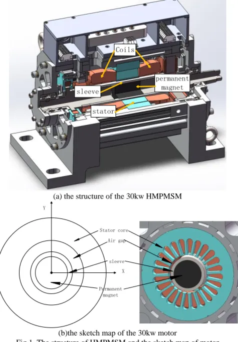
The structure of the 30kw HMPMSM shows in Fig.1(a),

The ECL optimization and experiment of HSPMSM with improved method

Xu Liu

1,2*

,

Member

,

IEEE

1

School of Instrumentation Science and Optoelectronics Engineering, Beijing University of Aeronautics and Astronautics, Beijing 100191, China

2

Beijing Engineering Research Center of High-Speed Magnetically Suspended Motor Technology and Application, Beijing University of Aeronautics and Astronautics, Beijing 100191, China

E-mail: [email protected]

consisting of motor, magnetic bearing, touchdown bearing, motor enclosure and other parts, in which the main loss generated in the motor part, consisting of stator, coils, sleeve wrapped outside of rotor, and permanent magnet, a cylinder embedded in the middle of it, comes down to the sketch map which is illustrated in Fig.1(b), of which the equivalent hierarchical model is left middle in Fig.1(b). The section of motor part of HSPMSM is in the right of Fig.1(b).

Coils

stator sleeve

permanent magnet

(a) the structure of the 30kw HMPMSM

Stator core Air gap

Permanent magnet

X Y

sleeve

(b)the sketch map of the 30kw motor

Fig 1. The structure of HMPMSM and the sketch map of motor The eddy current here we mainly consider the time harmonics which is produced by PWM modulation, ignoring the one generated by the spatial distribution of the windings and other spatial harmonics, such as tooth permeance harmonics.

The 30kw HSPMSM here, 48000r/min rated speed, mainly controlled by Three-phase six-step control strategy which permit two-phase simultaneous conduction.

With consideration of the ending effect, we compute the ECL by 3-d electromagnetic approach as the followings:

The structure of the motor, as is shown in Fig 1(b), in which the component of the rotor is stratified, including the sleeve and the permanent magnet, the magnetic field intensity and magnetic induction in every layer can be derived by Maxwell's equations, of which the component form is adopted.

First, five basic approximate assumptions are made here as the followings:

a.The current (magnetic potential) of stator three phase symmetrical windings is equaled by the line current on the stator inner surface. The effect of the stator tooth is analyzed with gap coefficient.

b.There is infinite length of the stator and the rotor, only the axial component considered.

c.Stator core unsaturated, of which permeability s  is

provided, while, the hysteresis influence of ferromagnetic material is negligible.

d.The orthogonal coordinate system is adopted, ignoring the curvature impact of the rotor, otherwise we may consume a lot of time in Bessel functions.

e.The fundamental component and those time harmonics in larger proportion would be calculated as like steady alternating field.

Based on those assumptions above, the general calculation model is illustrated as Fig.2. In coordinate system, x means circumferential direction,

x

_s means that is

fixed to stator,

x

_r is fixed to rotor, y means radial direction, and the z represents axial direction.

Above all. The coil current Jsz should be alternated by equivalent line current density located at the junction between the stator and air-gap, with sinusoidal distribution, transformed into Fourier series

as: 0,  

,

4 1

sin 1,3,5,...

k s j kp t ax

sz k

k v n r

n

J J e z n

n L







  

 _{ } 

 



(1)

1 0,

1

2 _{dp slot k}

k

K K N I J

D



 (2)

Where the Kdpis effective coil coefficient per phase of the

stator winding; Kslot is slot coefficient;

N

1 is number of turns; D1 represents inner radius of the stator; a

p





 ,

2 a

D p



 is the polar distance, where

D

a here is armature

diameter, namely the inner diameter of stator here; k and

v

are time and space harmonic order respectively. The related calculation expressions are listed as the followings:

0

0

sin 2

2

s slot

s b v

R K

b v

R

 

 

 

 (3)

where

b

₀ is slot width;

R

_s is inner diameter of stator.

dp pv dv

K



k

k

(4) Where the coil pitch coefficient

k

pv is:

sin

2

y pv

k







v











(5)

Where the



y is coil pitch angle.

The coil distribution coefficient

k

dv is:

1

1

sin

2

sin

2

dv

q

k

q































(6)

Where 1

2

p

Q







, the electrical pitch angle;

2

Q

q

mp



,

slot

Q



24

, phase number

m



3

, number of pole-pairs

1

p



.

z

y

x

stator

airgap

sleeve

Permanent magnet

1

,

1

 

2

,

2

 

3

,

3

 

4

,

4

 

Fig.2 the 3-D equivalent hierarchical model of motor The 3-D equivalent hierarchical model of motor and its conductivity and permeability in every layer is showing Fig.2.

The electromagnetic equations in every medium such as air-gap, sleeve and permanent magnet are listed as (7), (8), and (9) relatively:

2 2 2

2 2 2

0

g g g

A

A

A

x

y

z



















(7)

2 2 2

2 2 2

s s s

r s s s

A

A

A

j

A

x

y

z

  



















(8)

2 2 2

2 2 2

p p p

r p p p

A

A

A

j

A

x

y

z

  



















(9)

where the

A

g,

A

s, and

A

p is axial component of vector

magnetic potential. As the

A

_{p y}



C

,



s,



p are

conductivity of sleeve and permanent magnet respectively,

s



,



p are magnetic permeability respectively. Thus, the

solution of (10)-(12) can be listed as:





 11

sin k

j t ax

g gn n n n

n e

n

A C ch y D sh y e z

n L

 

    

  _{ }

 



(10)





 1

sin k

j s t ax

s cn cn cn cn

n e

n

A C cha y D sha y e z

n L

    

  _{ }

 



(11)

 

2

1

sin

n k

a y j s t ax

p n

n e

n

A

C e

z

n

L





 

















(12)

Where the

C

gn,

D

n,

C

cn,

D

cn and

C

2n are undetermined

constants. The other coefficients are: 1

2 ₂

2

2 2

cn k

r

n

a

a

jS

L



  



































(13)









 

3

3 2

2

k

j w t ax

cn cn n

cn

cn cn

a th

a l

a

D

e

th

a l

a









 





 

















(14)

1

2 ₂

2

3 3

n k

r

n

a

a

jS

L



  



































(15)

1 2 ₂ 2

n

r

n

a

L











 























(16)

To confirm the undetermined constants, the following

boundary and interface conations are listed as:

2 2

2 0 3 0

3 2

2 0 3 0

3 4

3 4

3 4

1

1

1

1

1

sz y g

y y

y y

y d y d

y d y d

A

J

y

A

A

A

A

y

y

A

A

A

A

y

y













 

 

 

 





























































(17)

where the d is the thickness of the

sleeve.

0 50 100 150

0.00 0.05 0.10 0.15 0.20 0.25 0.30 0.35 0.40

am

plitud

e o

f flu

x de

nsity(

T)

harmonic order Modulation and

commutation harmonics

Slot harmonics Coil distribution

harmonics

Fig.3 the harmonic component

The harmonic components, k-th order time harmonic and

the v-th order space harmonic, of air-gap flux density are

shown in Fig.3. The distribution harmonics, mainly

concentrate in 5,7,11,13th _{orders, resulting in 110W, as the} Fig.4 shows after all computation processes. Modulation

harmonics mainly concentrate in 160th _{order, occupying} little percentage, as the same as the slot harmonics, which

1W. However, the commutation harmonics, bringing about

197W ECL, occupies the largest percentage of total ECL.

Thus, the undetermined constants can be got via (13)-(17):

























2 0, 4 4 4 2 0, 2

4

4

n k gn cn cn

n n cn n

n

r cn cn n

cn

n cn cn

cn cn n

cn n

n n cn cn

a d

k cn cn cn

n

cn

n n cn n

n

J

C

C

a

sh

g

D ch

g

a th

a d

a

D

a th

a d

a

a th

a d

a

a

D

a th

a d

a

J e

ch

a d

D sh

a d

C

a

sh

g

D ch

g





































































 

















 

















































(18)

Where the 4

3 r









Substituting (18) into (10)-(12), the concrete expression of

2

A

,

A

₃,

A

4 and other electromagnetic terms can be got. For the sleeve, the axial component of the electric field intensity and the tangential component of the magnetic field intensity are the following expressions:





 

3

3 3 3 3 3

r r

j skp t ax

z r

A

E jskp C cht y D sht y e

t           (19)





  3 3

3 3 3 3 3

3 3

1

j skp _rt ax_r

x

A

t

H

C sht y

D cht y e

y



















(20) where,

1 2 3 , 3

3 1 2 3 2

sz k

K

J

C

aK shag

K chag

 



 

 



(21)

2 2 3 , 3

3 1 2 3 2

sz k

K

J

D

aK shag

K chag

 



 

 



(22)





2

3, 4,5

i r i i

t



a



jskpw

 

i



(23) The magnet thickness depends on its equivalent electromagnetic thickness, namely the thickest depth of penetration

d

4, whose expression is (30).

Thus, the expression of the ECL can be deduced by 3-d electromagnetic method from (28),

According to the complex Poynting power density method of sinusoidal magnetic field, the average power of one cycle current density vector, namely the average Poynting vector calculation formula is as the followings：

1

Re

2

av

S







E H













(24) Therefore, the average power density of the closed surface S is integrated to get the average electromagnetic power of the closed surface S:

1

Re

2

av s

P







E H









ds







(25) As long as the complex power

S

_3d has been obtained, as the (38), (39) shows:

4 5 3 5 3 4

1 4 4 4 4 3 4 4 4 4 3

5 4 5 3 4 3

K

 

sh d



ch d



ch l



 

ch d



 

sh d



sh l



 

 

 

































(26)

4 5 3 5 3 4

2 4 4 4 4 3 4 4 4 4 3

5 4 5 3 4 3

K

 

sh d



ch d



sh l



 

ch d



 

sh d



ch l



 

 

 

































(27)

 





 

2 2

1 0, 2

3 r,n,

2

, 2

4

k

k

j w t ax g k cn

r d k r r

k n k n cn cn cn cn j w t ax

n n n n

n n

jS

J

a D e

S

S

D L

a D

a D

n a

sh

g

ch

g

sh

g

e

ch

g

 

















 







 









 





 







(28)

    2 2 1 0, 2 2 2

2

k k

j w t ax g k c c

r d r r

j w t ax

k c c c c

jS

J

D e

S

D L

D

D

a

shag

chag

shag

e

chag

a

a

 









 







 







 





 





₍₂₉₎

where

4

0 4 4

1

d

f

  



(30)

The ECL caused by end of winding could be calculated by

subtracting

P

r d2 from

P

r d3 , which can be got from integrating by

S

r d2 and

S

r d3 , reaching about 24W showing in Fig.4





2

3 3 3 3

Re

r a r

skp

L

p

 

jC D t



 



(32)

Here, in order to get the end-effect factor, the 2-d formation of (29) and (31) are calculated in two-dimensional electromagnetic field, the similar expression of ECL by 2-d electromagnetic equation can be deduced, afterwards, the total rotor eddy current losses generated by motor can be got, and the difference between it and the one of the motor section calculated by subtraction between them, is just the eddy current loss of the winding end. When 2d electromagnetic field equation is utilized, the expression of the total complex power coming into the rotor surface is listed as formula (29). Besides, the compare of the 2d and 3d calculation results are shown in Fig.24.

The varieties of flux density harmonic component in air-gap that penetrate into the whole surface of the rotor,

generating corresponding ECL

P

_k, show in Fig.4

For the permanent magnet, the axial component of the electric field intensity and the tangential component of the magnetic field intensity are the following expressions:





 

4

4 4 4 4 4

r r

j skp t ax

z r

A

E jskp C cht y D sht y e

t



 



    

 (33)





 

4 4

4 4 4 4 4

4 4

1 j skp rt axr

x

A t

H C sht y D cht y e

y











  

 (34)

Thus, the Poynting vector that penetrate into the magnet is:







4 4 4

4

4 4 4 4 4 4 4 4 4

1 Re

2 2

Re

r

z x

y l y l

skp

S E H

jt C cht l D sht l D cht l C sht l

 



 

 

 

    

 

 

 _{ } 

 

(35)

So, the corresponding average electromagnetic power is:







2

4 4 4 4 4 4 4 4 4

3 Re r a m

skp L

P   jt C cht l D sht l D cht l C sht l



 

 

  _   _ (36)

So, the average electromagnetic power generated in sleeve is:

s r m

p



p



p

(37) The total ECL in sleeve is:

, sleeve s

k v

P





p

₍₃₈₎

,

mag m

k v

P





p

₍₃₉₎

Similarly, the

P

_r in permanent magnet can also be

deduced from the recurrence relation described as the above process accounting for the recurrence relation(15), (16) and solution(21) and (22) can still be applied in permanent magnet. The total loss result is listed in Fig.24 .

6

197

110

0.56 24 4

223

95

0.664 29

0 50 100 150 200 250

ending slot harmonic distribution

modulation

ECL(W)

ECL style

analysis(W) FEM(W)

motion

Fig.4 Comparison of various ECL between analysis and FEM

III. THE MULTI-OBJECTIVE OPTIMIZATION(MOO) OF THE ECL

Considering the different position, conductivity, temperature capability and the failure criteria, the different optimization weighting factor should be given to permanent magnet and the sleeve. A MOO method, which make use of the utilization method to limite the ECL here, accounting for those considerations can be adopted. The objective function can be expressed as:

 

 

1 1

2 2

sleeve

mag

F X P

F X P

 

 

 _

 (40)

The convergence evaluation function is listed as:

 

1

 

2

 

F X F X F X (41) Here we use the utilization method from [25]-[28]. The

1



and



2 form the utilization vector which ensures the optimization margin and constraints of every objective.

The optimization variables, listed in TABLE 2, are mainly from the structure parameters of the rotor, while the ones of the stator as the constrain, including the temperature limitation, via the air gap to contact with the ones of the rotor.

The constraints are:

1, The permanent magnet maximum demagnetizing working point under load condition should be guaranteed over the inflection point of the demagnetization curve:

The maximum demagnetization magnetic motive force of direct axis per-unit value

f

ad is:

0 0 0

1.35 2.7

2 ad 2 dp ad dp

ad h ad h

c c c

K NK K N

F

f I K I

F F p  pF

   (42)

where the maximum demagnetization current of direct axis

h

I

is :







2 2 2 2 2 2

0 0 1 0

2 2

1

d d d

h

d

E X E X R X E U I

R X

   



 (43)

Based on equivalent magnetic circuit computation, when

I

h

is injected in coils, the working point under load condition is:

(1 f )

1

1

1

ad

mn mn

n

n ad

mn mn

n

b

f

f

h









































(44)

Thus, the maximum demagnetization working point of permanent magnet is



b_mn,h_mn



,

satisfying the constraint:

mn k

mn k

b

b

h

h











(45) 2, The maximum temperature of each part among the motor should be below the allowable temperature with permitted allowance reserved.

T Ah

 

  (47)

where  is heat flux; A is area of dissipation; h is equivalent coefficient of heat conductivity or dissipation.

The heat source in every layer is the eddy current loss pn in every layer. Thus, the maximum temperature increase of the original HSPMSM model, calculated by equivalent thermal network method as Fig.5 shows, exists the outer surface of the sleeve, 96K.

Maximum temperature:130℃

Fig.5 Equivalent thermal network node graph (steady state) 3, Strength constraint of rotor sleeve:

The Von-Mises stress of sleeve



_vmh is:

2 2 2

1

(

)

(

)

(

)

2

h

vm rm m rm m



























(48)

which should satisfy the constraint:

max h h vm

n







(49)

where

 

rm

,

m are radial and tangential equivalent stress

respectively; the max 1146 h

Mpa



 is allowable limit of GH4169, the material of sleeve, with

n



1.3

, the safety coefficient.

4, Electric load constraint of winding:

1

0 1

dp

mNI K

A

A

p







(50)

Where

A

₀

 

7 10

5

A m

/

, the allowable limit of electric load with some allowance reserved.

5, Thermal constraint of winding:

1 1 0

AJ



AJ

(51)

1 1

1 2 2 2

11 12

1 2 2

2

2 2 t

t t

I I

J

d

d d _{a N}

a



N N



 

 _{   }  _{ }



 _ _ _ _  _ _

 

 

(52)

where

a

is number of parallel branches;

N

t is number of

wires per conductor;

d

is diameter of wire with its insulation.

2 3

1 0

650

/

AJ



A

mm

, the allowable limit of thermal load.

6, Constraint of spacer factor:

2

100%

t c c

a j

N

n

d

k

S

S

 







(53)

where

n

_c is number of conductors per slot；

S

a is area of

slot；Sj is area of slot insulation. According to the actual local level of wire assembly process of motor and the motor cooling requirements, the

k

c



70%

constraint.

7, length constraint of winding end:



'



2

E e

L  dl (54)

'

0

2 cos

y e

l





 (55)

' 0

sin

d e

f



l



(56) 2

1 2 0 2 1 2

2 2

s

i s s s

y

b

D h h h







 _{   } 

 

 

 (57)

max E

l



l

, where the

l

max



110mm

, the limit length of ending depends on the HSPMSM assembly.

8, length constraint of electromagnetic air-gap:

Here, with consideration of the cylindrical shape of the magnet, the air-gap flux density can be deduced by the following expression:

 



 





 



 





2

' '

0

0 1 '

cos cos

2

, , ; , ,

N

n k

k

MR

B S n n r R n

N

I r z R n z

    

 

 

 





_   _

(58)

which will be calculated in radial and circumferential direction respectively to get the total number.

2 4

max

2

1

10

em ef s

T





B L R A

_



 (59)

1 3

2 2 10

b s

b Fe pt B A

R 

 





 (60)

Thus, the electromagnetic air-gap



e satisfy the constraint:

0

e

R

s

R

m

R

h

R

m













(61) 9, length constraint of mechanical air-gap



m:

0

e m

R

s

R

h













(62)

10, Other geometric constraints

Thus, the constraint conditions in form of penalty function is used to construct the augmented objective function, which uses outer point method, the nonlinear constrained optimization problem is transformed into an unconstrained optimization problem with polynomial

penalty function, in which the

g

_i

(x)

is constraint,

u

_i

(g )

_i

is unit step function, ( )k

r

is penalty factor, which satisfy the following condition:

1 2 1

0

 

r

r

...

 

r

_k

r

_k

...

, the argumented objective function is:

 

 

 

(k) (k) 2

1

, r F r [g ] g

m

i i i i i

i

F X X X u



   

 



The unit step function

u

_i

(g )

_i is:

0, g (x) 0, (g )

1, g (x) 0,

i i i

i

if constraint is satisfied u

if constraint is not satisfied 



  _



(64)

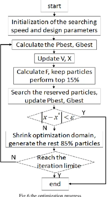
The optimization progress adopting above method by chaotic particle swarm optimization is illustrated as Fig.6.

Fig.6 the optimization progress

Chaotic particle swarm algorithm calculation process is shown in the Fig , the specific operation process is as follows:

1.Random initialization of the particle swarm: set the reliable population size, the initial position of the particle and the initial velocity, inertia factor and other parameters 2.Evaluate and compute the current adaptation value of

every particle; the position and the adaptive value of each particle are stored in the pbest of each particle, and the position and the adaptive value of the optimal individual in all pbest are stored in the gbest.

3.Update the current velocity and position of the particle according to the velocity and position function, the speed and position function is as follows:

 

 

 

 

, 1 , 1 1 1 , , 2 2 g, ,

i j i j i j i j j i j

v t wv t c r p_ x t _c r_p x t _

(65)

 

 

 

,

1

, ,

1 ,

1, 2,...,

i j i j i j

x

t

 

x

t



v

t



j



d

(66)

where weights w update under the following type adaptively:











max min min

min

min max

,

,

avg avg

avg

w w f f

w f f

f f

w

w f f

 



 

 _

 

 _



(67)

4.Calculate the objective function value of each particle, and then retain the best performance of the 15% particles in the group

5.In the population, the best particle in the swarm is searched, and the pbest and population of gbest are

updated. The search procedure is as follows:

(1) make k=0, The decision variables

x

k_j

,

j



1, 2,...

n

are mapped into chaotic variables

s

k_j varying in  0,1 _:

min, max,

, 1, 2,... k

j j

k j k

j j

x x

s j n

x x



 



(68)

Where

x

max,j and

x

min,j are the lower and upper bounds

for the j-th dimensional Searching variablerespectively. (2) Calculation of chaotic variables for the next iteration:





1

4

1

,

1, 2,...

k k k

j j j

s





s



s

j



n

(69) (3) Transform chaotic variable

s

k_j1 into design variable:





1 1

min, max, min,

,

1, 2,...n

k k

j j j j j

x





x



s



x



x

j



(70)

(4)Evaluate new solution according to design variable

x

k_j1: If new solution is better than initial solution which

is

X

(0)

 



x

1(0)

,

x

2(0)

....

x

n(0)





or the steps of chaotic searching progress reach top limitation of the iteration, set new solution as the result of chaotic searching progress, otherwise, change to step(2).

6.If the stop condition (preset convergence precision and maximum number of iterations) is satisfied, the searching progress stops and output results, otherwise, change to step 7.Contract search area under according to the followings:









min, min, , max, min,

x jmax x j,xg jr x jx j , 0 r 1

(71)









max, max, , max, min,

x jmin x j,xg jr x jx j , 0 r 1

(72)

Where

x

g j, represents the j-th dimensional design variable.

8.Compute the evaluation function F(x); if the expression

 

 

1

k k f

F  x F x 



is satisfied, iterations can be jumped as convergence.

9.The remaining 85% of the particles are randomly generated within the space of contraction.

After MOO optimization, the optimal design variables are listed as the following TABLE

Design parameters that exists in the design vector X is listed in TABLE 1 as the following form:

TABLE 1 the design parameters after optimization

Motor parameter Design variable

Design value Original optimal Rated power

（kW） 30 30

Rated voltage

（V） 480dc 480

Rated speed 48000r/min 48000r/min

Polar numbers 2 2

Slot numbers 24 24

Outer radius of

stator (mm) x1 150 178

Inner radius of

stator (mm) x2 62 67.6

Stator length

(mm) x3 60 60

Lamination factor

of stator 0.95 0.95

Stator material 20WTG1500 20WTG150

slot sketch

Slot notch height Hs0

(mm) 0.5 0.5

Slot shoulder height

Hs1(mm) 0.6 0.6

Slot body height Hs2 (mm) x4 20 24

Slot notch width Bs0(mm) x₅ 2 1.86 Slot upper width Bs1(mm) x₆ 4.9 5.6

Slot bottom width

Bs2(mm) x7 10.2 11.34

Rotor outer radius (mm) x₈ 55 59 Sleeve outer radius (mm) x₉ 55 59

Sleeve thickness (mm) x₁₀ 5 6.5

Magnet outer radius (mm) x₁₁ 45 46 Magnet axial length(mm) x₁₂ 60 60

Sleeve material GH4169 GH4169

Magnet thickness (mm) solid solid

Remanence (T) 1.05 1.05

Connection mode of

winding Y Y

Number of parallel

branches 2 2

Pitch 12 12

Conductor diameter (mm) 0.8 0.8

insulation thickness (mm) 0.06 0.06 Number of conductor per

slot 12 10

Number of wires per

conductor 8 10

Slot insulation thickness

(mm) 0.35 0.35

Layer insulation thickness

(mm) 0.35 0.35

Slot full rate(%) 41 42

Insulation grade H H

Axial length of the

winding end (mm) 50、60 49,58

The optimization performance is listed as the followings:

40 45 50 55 60 65 70 75 80 240

260 280 300 320 340

F2

F1

Fig.7 Pareto Front

The optimization point (258,77) is selected from Pareto Front as Fig.7 shows, accounting for other constraints requirements such as the strength, geometric and temperature increase.

The evaluation function converges after 51 iterations as Fig.8 shows. The ECL increase first, due to increase of the reluctance of air-gap, then decrease as the air-gap increase,

resulting from the increase of coil current gaining the upper hand, with air-gap continued increase, as Fig.9 shows.

0 10 20 30 40 50

290 300 310 320 330 340 350 360 370

F

iteration

F

Fig.8 Convergence curve of convergence evaluation function

6.5 7.0 7.5 8.0 8.5 9.0 9.5 10.0 10.5 11.0

338 340 342 344 346 348 350 352 354 356 358

ECL (W)

airgap (mm) ECL

Fig.9 ECL varying with air-gap

The ECL increase as the slot width increase, owing to more high order harmonics penetrating into the rotor from slot, as Fig.10 shows.

1.6 1.8 2.0

320 340 360

ECL (W)

slot width (mm) ECL

Fig.10 ECL varying with slot width

The sleeve plays the role of shield, of which the thickness increase leading to the ECL decrease of magnet, while, that increase of sleeve gains the upper hand as the sleeve thickness increase over 6.5mm.

5 6 7 8

280 300 320 340

ECL of

sleeve

(W)

sleeve thickness (mm) ECL of sleeve ECL of sleeve ECL of sleeve

40 60 80

ECL of

ma

gn

et

(W)

320 340 360 380

ECL of

ro

tor

(W)

IV. RESULTS VALIDATION VIA FEM

Here the finite element method(FEM) is used to validate the computation results got from above method.

First, the electromagnetic optimization results are validated by FEM. The control equation in eddy current generation field is:





=-0

A

A V A

t A

t

  

 

_{ } _{ } _{ } 

 

 _{  }

 

   

_{ }  _

    



(73)

The equivalent variation expression is:

 



 



0

F A A A d A Ad

t A A

    

 



 _{       }

 _

   





(74)

With proper boundary condition exerted in FEM model, the eddy current loss in total rotor of the original model is computed as 356.7W approximately as the Fig.12 shows:

Fig.12 the total ECL of the original rotor

(a)the ECL (b) the ECL density Fig.13 the ECL and the ECL density

Fig.14 the ECL of the optimal rotor

The total ECL of the optimal rotor is 294W, calculated by FEM, consisting of ECL in sleeve 237W and in permanent magnet 56.9W respectively, as Fig.14 shows, which has 12% error with the analysis results 335W.

Second, the thermal optimization results are examined by FEM as illustrated as the followings:

FEM process of three dimensional steady thermal field and fluid field of this PMSM deserves fundamentals of heat transfer, namely, with regard to analyzation of steady thermal field, steady heat conduction equation does not

contain the time term, meanwhile, including heat source and medium, which can be expressed under the Cartesian coordinate system as the shown below:

















,

, ,

0 , , Adiabatic Surface

, , Radiating Surface

x y z

f

T T T

k k k q

x x y y z z

x y z T

x y z n

T

k T T x y z n 

   _    _    _{ }

_{ } _ _{ }  _  _ _{ } _

 



 _



 _{ }

  

_  _{  }

 _



(75)

Where, T is temperature to be solved; K k k k



x, y, z



is thermal conductivity along each direction, W/(m.K); q is volume density summary of each heat source existing in solution domain, 3

/

W m ;  is surface coefficient of heat transfer, _W/



_{m K}2



; Tf is the temperature of fluid around

heat surface, K.

The fluid flow is governed by the laws of physical conservation, accounting for the fundamentals of fluid dynamics and heat transfer, the principle of mass, momentum and energy conservation are satisfied in the motor.When the fluid in motor is incompressible and flowing steadily, the corresponding three dimensional governing equations can be simplified as:









div

 

u



div



grad





S

(76) Where,



is general variable,



is the density fo fluid,

3

/

kg m ;



is spreading coefficient; S is the source term.

(a)the temperature of rotor (b) the temperature of motor Fig.15 the temperature of the motor

The highest temperature is 142℃ located in the positive center in cylindrical permanent magnet as Fig.15(a) shows. The biggest strength reached 478Mpa, satisfying the strength constraint of sleeve commendably, at the interface between between sleeve and permanent magnet showing in Fig.16(a).

(a) strength (b) strain Fig.16 the strength and strain of the rotor

(a) the prototype (b) the controller and driver Fig.17 the prototype and its controller

V. EXPERIMENT

The motor prototype is designed in the laboratory, and its electromagnetic losses are expressed in the form of heat, therefore, the total electromagnetic loss of the motor is equal to the heat generated by the motor excluding the windage loss in the unit time.

The total input power of the motor that the total input

electromagnetic power of the motor

p

_in can be tested by

power analyzer WT3000. The electromagnetic loss of the

motor

p

_e can be calculated as the followings:

e in f

p



p



p

(77) The

p

f is windage loss, which can be tested by draging

test showing in Fig.18

Output power analyzer

Water cooling Cooling fan

Temperature patrol instrument Motor-generator drag

system

Test line of input power analyzer

Magnetic bearing control system

motor control system

Motor Generator

Fig.18 the dragging experiment site

Fig.19 the sketch of the drag system First, when the motor reach the rated speed

The electromagnetic loss of stator consist of the core loss and the winding loss in which the effect of AC resistence should be considered, with the LCR analyzer as the Fig.22

shows its testing.

With the difference of loss component between the motor and the generator, the power composition of them is:

m m

m w fe e g

p



p



p



p



p

(78)

g g

g w fe e l

p



p



p



p



p

(79)

In equation (78),

p

_m is the input power of motor,

measured by power analyzer(Fig.24(a)).

p

_w is the windage

loss considering be the same value in both motor and

generator owing to the same speed of them,

p

m_fe is the core loss of the motor,

p

_em is the eddy current loss of the motor. In equation (79),

p

g is the input power of the generator,

g fe

p

and

p

_eg are core loss and eddy current loss of the generator respectively,

p

_l is the final load power. Since the

g fe

p

and

p

_eg in generator consist of sinusoidal fundamental component caused by the sinusoidal EMF owing to the parallel magnetization of the permanent magnet which can

be calculated by analytical method precisely. The

p

_m and

l

p

can be read from power analyzer. Then

p

m_fe and

m e

p

can be calculated by the following method:

The stator iron loss is measured by the testing instrument

of the TPS-500M which mainly measure the unit core loss

coefficient of silicon lamination steel in the laboratory as the

Fig.20 shows. The related correction factor is given by (60).

(a) the equipment (b)the test interface Fig.20 Test equipment iron loss and test interface of core loss per unit mass

of steel iron core lamination

0 100 200 300 400 500 600 700 800 900 0

100 200 300 400

loss p

er

un

it ma

ss (W/kg

)

Frequency (Hz) 0.2T

0.4T 0.6T 0.8T 1T 1.2T 1.4T 1.5T

The steel iron core, made of 20WTG1500, whose testing

results of core loss per unit mass of steel iron core

lamination shows in Fig.21, in which the loss per unit mass

curve is fitted by BP method.

According to the characteristics of the mechanical loss of

the magnetic suspension motor in the laboratory, a method

to calculate the iron loss by the power coefficient method is

presented, based on the phase voltage measurement. The

separation results generated by the traditional method

according to the test standard of the International Electrical

Commission IEC60034-2: under constant speed load, the

power value P and

U

2 displaying on the power analyzer that is recorded. The method is suitable for low speed (more

slowly than 10000r/min), which can be used for PWM

control strategy of the core loss measurement.

Only when the fundamental action is considered, owing to:

3 dc

f U

Bf C

 

   (80)

Iron loss caused by Fundamental magnetic density can be

expressed by the following formula:

2 2

h e h e

C

P P P k k C

f

    (81)

So the traditional method with curve P and 2

U

intercept

approximation to calculate wind friction loss and iron loss,

the traditional iron loss formula:

 





_{2 2}





1.5

1

a

h m c m a m

P



k



K



B

fB



k f B



k B f

(82)

In above formula,

 

1

n

p i

i

D

K B

B B

  





, generally, D=0.65;

the loss coefficients can be got by BP fitting method as

Fig.21 shows:

0.271; 0.698; 1.6

172.716; 2

h c e

K  K  K 





The high frequency characteristic and the high frequency

loss of high speed motor are mainly composed of 3, 5, 7 and

9 harmonic orders, which is D=0.73

The core loss with this modification method is 295W in

55000r/min, while with original method 278W.

The principle of measuring total AC resistance is: 2

1 2 1 n

i i ac dc

n i i

I

K R R

I n n





 







(83)

c a

R



R K

(84) In above formulas, Ii is every harmonic current,

R

a is

direct resistance, while

R

_c, is AC resistance, measured by

testing method as Fig.22 shows, of which the measurement results showing in Fig.23. AC resistance has slow growth before 1kHz, while the AC inductance has smaller changes, however, which has sudden change in initial increase stage of frequency.

(a) the LCR instrument (b) the coils embedded in stator

Fig22. the site of measurement of AC resistence

0 1000 2000 3000

20 40 60 80 100

frequency (Hz) resistence_U inductance_U resistence_V inductance_V resistence_W inductance_W resistance_individual wire inductance_individual wire

192 193 194 195 196

20 40 60 80 100

194 196

20 40 60 80 100

192 193 194 195 196

400 600 800 1000 1200

250 252 254 256 258 260 262 264

Fig.23 measurement results of AC resistance and inductance

The effective value of the phase current of the oscilloscope

can be calculated, so the AC armature loss

p

_a, is 93W at

55000r/min rotation speed, can be calculated as:

2 2

2 2

a p c k ck

k

p  I R 



I R ₍₈₅₎

where

R

_c has been illustrated and measured by (83)-(84).

Thus, the electromagnetic loss of the rotor is the total

electromagnetic loss minus the total loss of the stator:

r e s

p  p p (86)

(a) full load (b) whole motion course

Fig.24 display of the full load and whole motion course

During the whole load process, the display of oscilloscope

arranged as the followings:

15000 20000 25000 30000 35000 40000 45000 50000 55000 60000

0

5

10

15

20

25

30

inpu

t p

ower

of

th

e m

oto

r(

kw)

speed(r/min)

input power of the motor(kw) phase current of motor(A) phase current of generator(A) output power of generator（kw） phase voltage of motor(V) phase voltage of generator(V)

50

100

150

200

ph

ase

volta

ge

of

mo

tor

(V)

10

20

30

40

50

60

ph

ase

cur

re

nt

of

mo

tor

(A)

50

100

150

200

ph

ase

volta

ge

of

ge

ne

ra

tor

(V)

0

20

40

60

ph

ase

cur

re

nt

of

ge

ne

ra

tor

(A)

-2

0

2

4

6

8

10

12

14

16

18

20

22

24

26

28

30

ou

tpu

t p

ower

of

ge

ne

ra

tor

（

kw

）

Fig.25 measurement data during whole loading process

26500 27000 27500 28000 28500 29000 29500 30000

0.2 0.4 0.6

P

Linear Fit of Sheet1 B"P"

P(kw)

U^2(V^2)

Equation y = a + b*x Weight No Weighting Residual Sum of Squares

0.12426 Pearson's r -0.15224 Adj. R-Square -0.46524

Value Standard Error P

Intercept 0.94448 2.68488 Slope -2.13104E-5 9.78273E-5

Fig.26 wind friction separation based on searching the negative slope

mutation point

30220 30240 30260 30280 30300 30320 30340 30360 30380 30400 30.96

30.98 31.00 31.02 31.04 31.06 31.08 31.10 31.12

31.14 P _{Linear Fit of Sheet1 B"P"}

P(kw)

U^2(V^2)

Equation y = a + b*x Weight No Weighting Residual Sum of Squares

0.00167 Pearson's r 0.95733 Adj. R-Square 0.88865

Value Standard Error P Intercept 0.95596 5.25032 Slope 9.93531E-4 1.73154E-4

Fig.27 the fitting result of the wind friction separation

The wind friction loss should be separated by

P U

-

2

relation curve method to get the intercept by fitting the data

point which is obtained from power analyzer(whose

corresponding display interfaces located in corresponding

points relatively nearby, showing in Fig.26)

The traditional method is searching the key point which

leading the curve fit to the one with negative intercept,

which method has weakness that the point that leading to fit

the curve to the one with negative slope, which is often

located in front of the former, make the curve deviation

from the actual. Thus, the improved fitting method,

searching the key point that lead to the curve fit to the one

with negative slope, is utilized to fit the curve(Fig.27). The

first point that generate the negative slope, afterwards, the

points that located after that are retained, which are used for

fitting the genuine curve. The wind friction loss(WFL) is

956W after improved fitting process, which corresponds to

the result 865W, generated by traditional fitting method.

The simulation result is 1161W generated by CFX.

The wind friction loss separation result at the speed of

55000r/min is listed as the following diagram:

82 93 93

245368 278410 295387 1161

865 956

1865

1646 1731

simulation experiment improved fitting mthod 0

500 1000 1500 2000 2500

winding

loss (

W)

three loss-apartment method winding loss stator core loss rotor eddy current loss windage loss total loss

Fig.28 compare of the loss separation results

As Fig.28 shows, ECL in rotor separated by improved fitting method reaches 387W, which is more close to the temperature increase, when used for heat resource in CFD, of rotor surface measured in the following steps. Besides, WFL occupies the largest percentage, play the main heat source of rotor in high speed working condition, so, WFL should be considered in next optimization.

Related computation, simulation and experimental results show as the followings, which shows the ECL varieties by rotation speed:

0 10000 20000 30000 40000 50000 60000

0 50 100 150 200 250 300 350 400 450

ECL (W)

ratation speed (r/min) ECL(by equivalent hierarichal method) ECL(3d EM computation)

ECL(2d EM computation) ECL(experimental) ECL(FEM)

Fig.29 the diagram of ECL data changing with rotation speed via various analytical, simulation and experimental method

and some performance prediction of HSPMSM. The equivalent hierarchical method listed in Fig.29 is dividing sleeve and permanent magnet into many thin layers to avoid curvature effect resulted from rectangular Cartesian

coordinate system.

The temperature of rotor surface is measured by infrared radiation thermometer as the Fig.30(a) shows, with the upper cover left, as the Fig.30(b) shows, immediately, just right as the HSPMSM stops operating.

(a ) infrared radiation (b) site of measurement thermometer of rotor surface temperature Fig.30 the site of measurement of rotor surface temperature

Coils

infrared radiation thermometer

sleeve

Measurement point stator

rotor

Fig.31 the sketch of measurement of rotor surface temperature

The temperature rise of rotor surface is given in Table2 Table2 Test measurement results of rotor surface temperature rise at stable

running of 48000r/min

speed 48000r/min

Axial ventilation × √ √ ×

Water cool × × √ √

Rotor temperature

increase 95K 9K 8K 89K

The temperature rise of the rotor surface is measured by

infrared radiation thermometer, reaching 95K+28K (ambient

temperature). The temperature rise of the other part of the

motor body is measured by thermistor PT100, whose

placement location is showing as:

5 7 3 1 2 4 8 6

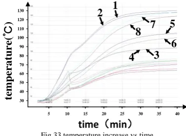
Fig. 32 Probe position of thermal resistors in high-speed machine and temperature rise curve

The maximum temperature of HSPMSM exists in coils, which has F-level insulation, and stators, reach 131℃ and 128℃ respectively. After adding water cooling, the temperature can decrease more than 19℃ at least. Besides, the temperature of rotor surface, with the slot surface, holds

less than 125℃, which keeps sleeve’s strength and magnetic performance of permanent magnet safe.

time

（

min

）

te

m

p

e

r

at

u

r

e

(

℃

)

5 10 15 20 25 30 35 40 30

40 50 60 70 80 90 100 110 120

130

1

2

7

8

6

5

3

4

Fig.33 temperature increase vs time

The temperature measured by those PT100, embedded as Fig.32 shows, is showing in Fig.33. The highest temperature rise in motor is iron core, the next is the inner surface face to the rotor surface.

VI. THE RESULTS AND CONCLUSIONS

The loss is less 17% than the original one after MOO process, decreasing from 356.7W to 294W, with appropriate treatment of the conflict among the sleeve thickness, outer diameter of rotor and air-gap length. The maximum temperature in sleeve and the permanent magnet is also less 11% and 16% respectively than the original design model. Both of the above results are all configured by FEA and tests. Though, the ECL results calculated by the 3-d electromagnetic method is closest to the experiment, so the expression of the ECL generated from that method should be better chosen as the optimization objective model, which can be improved in follow-up improvement.

Ⅶ.ACKNOWLEDGEMENT

SUPPORTED BY THE FUNDAMENTAL RESEARCH FUNDS FOR THE CENTRAL UNIVERSITIES. NATIONAL NATURE SCIENCE FOUNDATION OF CHINA:61573032, 61421063 AND 61403015.

References

[1] Yulong, L. Xing, L. Yi and C. Feng, "Effect of air gap eccentricity on rotor eddy current loss in high speed PMSM used in FESS," Electromagnetic Launch Technology (EML), 2014 17th International Symposium on, La Jolla, CA, pp. 1-6, 2014.

[2] A. Hemeida, P. Sergeant and H. Vansompel, "Comparison of Methods for Permanent Magnet Eddy-Current Loss Computations With and Without Reaction Field Considerations in Axial Flux PMSM," in IEEE Transactions on Magnetics, vol. 51, no. 9, pp. 1-11, 2015.

[3] F. Dubas and A. Rahideh, "Two-Dimensional Analytical Permanent-Magnet Eddy-Current Loss Calculations in Slotless PMSM Equipped With Surface-Inset Magnets," in IEEE Transactions on Magnetics, vol. 50, no. 3, pp. 54-73, 2014.

[4] X. Yongxiang, Y. Qingbing, Z. Jibin and W. Hao, "Influence of periodic carrier frequency modulation on stator steel core loss and rotor eddy current loss of permanent magnet synchronous motor," Electrical Machines and Systems (ICEMS), 2014 17th International Conference on, Hangzhou, pp. 2094-2100, 2014. [5] K. H. Kim, H. I. Park, S. M. Jang, D. J. You and J. Y. Choi,

"Comparative Study of Electromagnetic Perfor