Single Channel auditory source separation with neural network

(1)

Single Channel auditory source separation

with neural network

Zhuo Chen

Submitted in partial fulfillment of the requirements for the degree of Doctor of Philosophy

in the Graduate School of Arts and Sciences

COLUMBIA UNIVERSITY 2017

(2)

(3)

c 2017 Zhuo Chen Some Rights Reserved

This work is licensed under the Creative Commons Attribution 4.0 License. To view a copy of this license, visithttps://creativecommons.org/licenses/by/4.0/or send a letter to Creative Commons, 171 Second Street, Suite 300, San Francisco, California, 94105, USA.

(4)

(5)

Abstract

Single Channel auditory source separation with neural network

Zhuo Chen

Although distinguishing different sounds in noisy environment is a relative easy task for human, source separation has long been extremely difficult in audio signal processing. The problem is challenging for three reasons: the large variety of sound type, the abundant mixing conditions and the unclear mechanism to distinguish sources, especially for similar sounds.

In recent years, the neural network based methods achieved impressive successes in various problems, including the speech enhancement, where the task is to separate the clean speech out of the noise mixture. However, the current deep learning based source separator does not perform well on real recorded noisy speech, and more importantly, is not applicable in a more general source separation scenario such as overlapped speech.

In this thesis, we firstly propose extensions for the current mask learning network, for the problem of speech enhancement, to fix the scale mismatch problem which is usually occurred in real recording audio. We solve this problem by combining two additional restoration layers in the existing mask learning network. We also proposed a residual learning architecture for the speech enhancement, further improving the network generalization under different recording conditions. We evaluate the proposed speech enhancement models on CHiME 3 data. Without retraining the acoustic model, the best bi-direction LSTM with residue connections yields 25.13% relative WER reduction on real data and 34.03% WER on simulated data.

Then we propose a novel neural network based model called “deep clustering” for more general source separation tasks. We train a deep network to assign contrastive embedding vectors to each time-frequency region of the spectrogram in order to implicitly predict the segmentation labels of the target spectrogram from the input mixtures. This yields a deep network-based

(6)

analogue to spectral clustering, in that the embeddings form a low-rank pairwise affinity matrix that approximates the ideal affinity matrix, while enabling much faster performance. At test time, the clustering step “decodes” the segmentation implicit in the embeddings by optimizingK-means with respect to the unknown assignments. Experiments on single-channel mixtures from multiple speakers show that a speaker-independent model trained on two-speaker and three speakers mixtures can improve signal quality for mixtures of held-out speakers by an average over 10dB.

We then propose an extension for deep clustering named “deep attractor” network that allows the system to perform efficient end-to-end training. In the proposed model, attractor points for each source are firstly created the acoustic signals which pull together the time-frequency bins corresponding to each source by finding the centroids of the sources in the embedding space, which are subsequently used to determine the similarity of each bin in the mixture to each source. The network is then trained to minimize the reconstruction error of each source by optimizing the embeddings. We showed that this frame work can achieve even better results.

Lastly, we introduce two applications of the proposed models, in singing voice separation and the smart hearing aid device. For the former, a multi-task architecture is proposed, which combines the deep clustering and the classification based network. And a new state of the art separation result was achieved, where the signal to noise ratio was improved by 11.1dB on music and 7.9dB on singing voice. In the application of smart hearing aid device, we combine the neural decoding with the separation network. The system firstly decodes the user’s attention, which is further used to guide the separator for the targeting source. Both objective study and subjective study show the proposed system can accurately decode the attention and significantly improve the user experience.

(7)

List of Figures

2.1 The ideal ratio mask . . . 7

2.2 Different rules in speech spectrograms . . . 8

2.3 The NMF working pipeline . . . 11

2.4 An example for NMF decomposition . . . 12

3.1 The feedforward network and recurrent network . . . 16

3.2 The Pipe line for noisy auto encoder . . . 21

4.1 Feature mapping and mask learning . . . 24

4.2 The CHiME 2 speech enhancement evaluation . . . 26

4.3 Architecture of the extended mask learning with pre- or post- restoration layers 28 4.4 Architecture of the residue-learning based speech enhancement model . . . . 30

4.5 Speech recognition accuracy performance with residual learning . . . 34

5.1 The permutation problem and the output dimension mismatch problem . . . 38

5.2 Example of three-speaker separation . . . 44

5.3 Scatter plot for the input SDRs and the corresponding improvements . . . 51

5.4 Example spike-triggered spectrogram averages with 50-frame context . . . 52

6.1 The system architecture for deep attractor network . . . 55

6.2 Location of T-F bins in the embedded space . . . 57

6.3 Location of attractor points in the embedding space . . . 59

7.1 Structure of the Chimera network . . . 63

7.2 Example of separation results for music separation . . . 67

7.3 A schematic of our proposed system . . . 69

7.4 DNN output correlation analysis . . . 78

7.5 Decoding accuracy analysis . . . 80

7.6 Dynamic switching of attention . . . 81

7.7 Dynamic switching of attention results 2 . . . 82

7.8 Psychoacoustic Results . . . 83

(12)

(13)

List of Tables

4.1 Speech recognition word error rate (WER) comparison mask learning with/without scale restoration . . . 32 4.2 Speech recognition WER performance comparison for feature mapping . . . . 32 4.3 Speech recognition accuracy comparison for residue learning . . . 33 4.4 Speech recognition accuracy performance comparison for single-channel

far-field speech enhancement using bLSTM with input residue connection . . . . 34 5.1 SDR improvements (dB) for different separation methods . . . 43 5.2 SDR improvements (dB) for different embedding dimensionsD and activation

functions . . . 43 5.3 SDR improvement (dB) for mixtures of three speakers . . . 44 5.4 SDR (dB) improvements using the ideal binary mask (ibm), oracle Wiener-like

filter (wf) . . . 49 5.5 Decomposition of the SDR improvements (dB) on the two-speaker test set . 49 5.6 SDR (dB) improvements on the two-speaker test set for different architecture

sizes . . . 49 5.7 SDR (dB) improvements on the two-speaker test set after training with 400

frame length segments . . . 50 5.8 Generalization across different numbers of speakers . . . 50 5.9 Performance as a function of soft weightedK-means parameters . . . 50 5.10 SDR / Magnitude SNR improvements (dB) and WER with enhancement

network . . . 51 6.1 Evaluation for networks with different configurations . . . 60 6.2 Evaluation results for three speaker separation . . . 60 7.1 Evaluation metrics for different systems in MIREX 2014-2016 on the hidden

iKala dataset . . . 66 7.2 SDRi (dB) on the DSD100-remix and the public iKala datasets . . . 66 7.3 The number of electrodes retained for each frequency band and each patient. 73

(14)

(15)

List of Abbreviations

• FFT - Fast Fourier Transform • DFT - Discrete Fourier Transform • STFT - Short Time Fourier Transform

• CASA - Computational Auditory Scene Analysis • NMF -Non Negative matrix factorization

• DNN - Deep Neural Network • RNN - Recurrent Neural Network • ASR - Automatic Speech Recognition • SE - Speech Enhancement

• AE - Auto Encoder • DC - Deep Clustering

• DAnet - Deep Attractor Network

• MIREX - Music Information Retrieval Evaluation eXchange • LSTM - Long Short Term Memory

• BLSTM - Bi-directrional Long Short Term Memory • SDR - Signal to Distortion Ratio

• SIR - Signal to Interference Ratio • SAR - Signal to Artifact Ratio • SNR - Signal to Noise Ratio

• MMSE - Minimum Mean Square Estimators • PESQ - Perceptual Evaluation of Speech Quality • RMS - Root Mean Squared

• SGD - Stochastic Gradient Descent

(16)

(17)

Acknowledgments

This thesis is dedicated to my wife Jie and my daughter Claire. Jie, I feel so lucky that I can have you accompanied for the journey of my PhD, I love you. Claire, having you is the best thing that happened to me.

A special thanks to my parents, I can’t even count how much help I received from you. It is your selfless love and help that led me to where I am. I’d like also to express my gratefulness to my parents-in-law. Without your help to take care of Claire, I would need at least another two years to finish my PhD, thank you so much!

Being very fortunate, I had a chance to work with Professor Dan Ellis during my master in 2011. From this opportunity, I started my career in audio research. Dan, words can’t express my gratefulness to you. It is you who led me into this exciting field and I can always remember each guidance and help from you, Thank you so much!

After starting my PhD in 2012, I had the opportunities to get in touch with many professors. They are all very kind and from them I built a concrete background for my later research. Here I’d like to thank them all. Among them I’d like to specially express my gratefulness to Professor John Wright, who taught me in three different classes, where I extend the course project to my first publication.

In LabROSA, I am happy to meet and collaborate with many friends, who are all great researchers. Not only I learnt different perspective in research from them, more importantly, the time we spend together helped me to understand and adopt the entirely different culture in US. Colin, Dawen, Brian, H´el`ene, Byung Suk, Matt, Thierry, Courtenay, Rachel, Cyril, Diego, Minshu, James, Andy, and Douglas, thank you!

In 2014, I started an eight-month internship in Mitsubishi Electric Research Lab in Cambridge, which is definitely one of the most exciting experience in my life. Together with John, Shinji, Jonathan and Hakan, we made so many exciting works and I benefited so much from the collaborations, meetings and even casual chats. Here I would like to express my deepest appreciation to them. And I want to also thank my dear friends in MERL, Scott, Umut and Takuya, for the constructive discussions and the fun we had.

Then I had another three-month internship in Microsoft in Bellevue, which is also extremely beneficial. Although the time is short, with the help of my colleagues and friends there, we made full use of it. Those memory there is so nice that I decide to join Microsoft as my next stop after PhD. Jinyu, Yan, Yifan, Shixiong, Yong, Qiang, Min, Kaisheng, Yun, thank you for all the help and let’s build something greater together!

(18)

In early 2016, I started the collaboration with Professor Nima Mesgarani, who is extremely talented and helpful. With this help, I start to actually unveil the mystery of deep network. Here I’d like to express my very special appreciation to Nima. Nima, thank you so much and I am sure we can keep making great work together even after I graduate. And I’d also like to express my thanks to my labmates in NAPlab. It is the first time in my life to study in a place where there are more girls than men. Tasha, Bahar, Laura, James, Rashida, Prachi, and Hassan, I always enjoyed the atmosphere the collaboration and the conversation we had, thank you so much! And a special thanks to Yi, who I have the honor to mentor since 2016, I am impressed by your altitude and efficiency.

And I’d like to thank all my friends in New York and China, thanks a lot for the support and the fun we had.

Finally, it might be a little strange, but I’d also like to express my appreciation to all the researchers in this field. I am always exciting to read the new and cool works you made. Thank you for all of your excellent works that opened this exciting era in artificial intelligence.

(19)

1

Chapter 1

Introduction

The world is filled with an extremely large variety of sound. Most of the audio that human percept daily contain more than one audio source. For example, the average ambient noise in quite rural area is 30dB. And in more noisy cases, such as car. The noise level can reach 77dB(acoustics,2016). Fortunately, human is especially good at separating the mixed sound. It is a natural gift for human to separate target sound under even very challenging environment. For example, even a child could easily distinguish and understand the voice of their parents, in very noisy environment such as restaurant and street.

More impressively, the whole separating process in brain is usually performed uncon-sciously(Mesgarani and Chang,2012). Most people rarely notice the separating process. And the study showed that the separation could be largely enhanced when the attention is paid on specific sources(O’Sullivan et al.,2015a).

A natural question arisen, can this process be modeled with mathematical model? Solving the audio separation could not only help to build a better understanding for both audio signal and human brain, more importantly, it also has great practical value. The most obvious example is automatic speech recognition. Nowadays the best automatic speech recognition(ASR) system can reach human level performance when tested in matched conditions(Xiong et al.,

2016b;Amodei et al.,2015). When tested under more complex environment, however, the recognition error rate increased greatly (Amodei et al., 2015). In recent years, as home intelligence becoming popular such as Amazon echo, further demand for robustness is required because usually the distance between the speaker and the sensor is much larger than the traditional ASR applications in cell phone. And the ability for noise and reverberation removal is even more important. In some other applications, the separation itself is the main feature, one such example is on music, where the task is to separate each instrument, which can be further used in applications such as audio resynthesis or karaoke.

(20)

1.1 background 2

1.1

background

Inspired by the observation on human and the practical demand, researchers started the odyssey for searching computational models for audio source separation in very early age of modern digital signal processing. In 1950s, the “cocktail party problem” was first introduced by Colin Cherry(Cherry,1953), where the task was to separate each individual speaker in a cock-party, when all participant are talking simultaneously. Unfortunately, though the task seems easy for people, when researchers tried to build mathematical model to simulate the process, they found it was surprisingly difficult.

The problem of audio source separation is generally divided into two categories, multi-channel separation and the single channel source separation, where the number of the sensor(micro-phones) applied in the signal recording are different. Since the multi channel recording contains more than one sensor, the spatial information for each source can be inferred based the on time delay between microphones, i.e. the beamforming process(Fischer and Simmer,

1996;Anguera et al., 2007;Benesty et al.,2007;Kellermann,1997). And this information provides extra clue for separation. In this thesis, we mainly focused on single channel recording, which is more challenging but common in real world scenarios.

In past six decades, different models were proposed, which can be roughly divided into signal processing based methods(Ephraim and Malah, 1985; Hu and Loizou,2008,2007), rule based methods(Brown and Cooke, 1994; Wang and Brown, 2006; Ellis, 1996b), and decomposition based methods(Raj et al.,2010;Chen and Ellis, 2013;Schuller et al.,2010). Unfortunately very few of them could achieve robust and high quality separation. In recent years, with increased data amount and stronger computational power, the deep neural network(DNN) based system brought revolution to this long stand problem. The DNN based systems significantly increased the separation performance for speech and noise. More impressively, by special design(Chen et al.,2016;Isik et al.,2016b;Hershey et al.,2016b;Yu et al.,2016), the DNN also demonstrates the ability to separate more challenging mixtures, such as unknown number of overlapped speakers. The successes with DNN model provided important steps towards eventually solving the cock-tail party problem.

1.2

Contribution

In this thesis, the problem of single channel audio source separation is analyzed and discussed in depth. The previous models proposed for this problem are systematically reviewed. We also introduce two extensions for deep neural network based speech enhancement system, which provided significantly better result for both separation and the recognition of the noisy speech.

We introduce two novel neural network - based models, deep clustering(DC) and deep attractor network(DAnet ), which are designed for more general source separation problem, when the mixing sources are from similar sound families(within family separation), e.g. speech vs. speech, other than just speech vs. noise(cross family separation). In within family separation, we show that the separation is limited by two major difficulties, the permutation problem and the output mismatch problem. In deep clustering, the two problem was solved by using a clustering based objective function. This objective function also allowed the

(21)

1. Introduction 3

system to have many attractive features such as number of source invariance. We showed that DC outperformed the previous state of the art the by more than three times, and decreased the word error rate for recognition from 89.81% to 30.12%.

The deep attractor serves as the updated version of deep clustering, which enables several advantageous properties such as end-to-end optimization, flexible objective, reduced com-putational complexity etc. We discuss several variations of the DAnet, and show that the DAnet can provided even better result than DC.

We introduce two applications using the proposed model–the neural attention guided sep-aration and music sepsep-aration. In neural attention guided sepsep-aration, the attention of the patient is firstly decoded from the neural signal collected with an invasive sensor, which controls the separation process for specific source. This application provide an important practice for the next generation of hearing aid devices. In music separation, we combine the DC and a classification objective, and achieve the state of the art performance in singing music separation. And we show that even under highly mismatched condition, the system can robustly separate the sining voice and background music with high quality.

Finally, we provide the code and a application program interface(API) for all the proposed system in this dissertation.

1.3

Overview

The thesis is organized as follows: background material about source separation is presented in Chapter2. In Chapter3, a brief introduction on feedforward and recurrent neural networks is given, with emphasize on the application in audio processing. The neural network based speech enhancement system is described in Chapter4, where several aspects from modeling to implementation are discussed. In Chapter5and Chapter6, the deep clustering and deep attractor network are introduced in detail. Chapter7 and describes the applications of the proposed model. Finally the possible extensions and further works are discussed in the last chapter8.

(22)

1.3 Overview 4

(23)

5

Chapter 2

Background

In this chapter, we introduce several basic aspects of signal channel audio source separation, including basic concepts and background methods.

2.1

Audio mixture

Since the sound is fundamentally the energy in medium, the mixture of the sound is the summation of the energies from individual sources. Mathematically, this relation can be represented as (2.1), where y(t) is the audio mixture at time t and xi(t) refers the ith

individual source.

y(t) =X

i

xi(t) (2.1)

After recorded with microphone, the signal is usually discretized by sampling, while the additivity remains, which leads to (2.2), wherenis used to represent each individual sample. And we usually refer this representation as time-domain representation.

y[n] =X

i

xi[n] (2.2)

Though recently several new works(Li et al.,2016;Sainath et al., 2015b,a) showed that the model directly build in time domain could lead good performance in speech recognition and synthesis, the Fourier analysis is most commonly applied for audio processing. In Fourier analysis, the time domain signal is projected into a space that are support by the sinusoid functions with different frequencies, shown in (2.3), whereXi andY are transformed single

sources and the mixture.

Y(ω) =X

i

X(ω) (2.3)

When processing with long time series signal, such as audio. The time domain signal is often divided into overlapped segments, and then processed with Fourier transform separately.

(24)

2.2 Mask 6

This process is called short time Fourier transform(STFT). Since the Fourier transform is linear, the additivity remains, resulted in (2.4), where X and Y are the transformed time domain signal. The transformed representation is referred as spectrogram, and frame and bin are used to refer the time index t and frequency index f in spectrogram. Each number in spectrogram is known as T-F bin. We refer this spectrogram as frequency-domain representation.

Y(f, t) =X

i

Xi(f, t) (2.4)

Since the Fourier transformation often results in complex values, the magnitude, phase and power of spectrogram are referred as magnitude spectrogram, phase spectrogram and power spectrogram, accordingly. Study showed that phase is not very informative(Schluter and Ney,2001), and since it is more difficult to process complex number, the phase information is usually discarded. Magnitude spectrogram or power spectrogram are usually selected for further processing. Such procedure would break the additivity, but when the mixing sources are not correlated, the additivity could be approximately preserved, as suggested in (2.5). Moreover, for applications in speech recognition, study showed that removing phase would not affect the recognition performance.

|Y(f, t)| ≈X

i

|Xi(f, t)| (2.5)

2.2

Mask

The mask is one of the most commonly used the representation in audio separation. As its name suggests, a maskM in_RF×T _{is a matrix that can applied on the mixture spectrogram,}

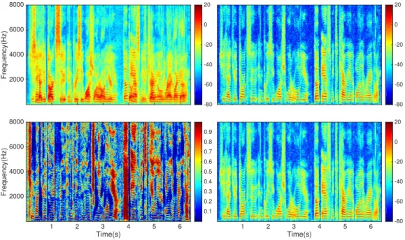
by point-wise multiplication, to mask out the interference for the target source. Depend on the choice of the value, the mask can be roughly divided into three type: Binary mask, Ratio mask and Complex mask. In binary mask, each TF-bin in mask has the binary value, which means each TF bin can only belong to one source. Such mask is usually easier to optimize but has worse separation. In contrast, in ratio mask the elements have continuous value between 0 and 1, i.e. the soft assignment for each TF bin. In complex mask, all the elements have complex value, which could be directly applied on the complex mask. An example of mask is shown in fig 2.1. In fig2.1, we can see that the ideal ratio mask can generate almost perfect separation.

(25)

2. Background 7 Frequency(Hz)₂₀₀₀ 4000 6000 8000 -80 -60 -40 -20 0 20 Time(s) 1 2 3 4 5 6 Frequency(Hz)₂₀₀₀ 4000 6000 8000 0.1 0.2 0.3 0.4 0.5 0.6 0.7 0.8 0.9 Time(s) 1 2 3 4 5 6 -80 -60 -40 -20 0 20 -80 -60 -40 -20 0 20

Figure 2.1: Upper left: The spectrogram of the the mixture between a male and a female speaker. Bottom left: The ideal ration mask for the female speaker. Upper right: The clean speech for the female speaker. Bottom right: The masked mixture.

2.3

Signal processing based source separation

In signal processing based source separation was mainly designed for speech enhancement, and was the first algorithm family proposed for this problem, in early 1970s. In this algorithm family, speech is usually assumed to follow specific distribution such as Gaussian or Laplacian. Then a maximum likelihood model is build based on this assumption. The noise is assumed to be stationary, whose statistical properties don’t change through time. In practice, a voice activity detector is usually applied to noisy speech first, then the silent frames are collected to calculate the noise statistics, followed by the maximum likelihood optimization to get the speech.

Since most of the signal processing based model make over simplified assumption on speech, e.g. following gaussian distribution, and those method are not date driven, which means that the system could not learn from the actual data, the performance of signal processing based method are usually unsatisfiable and will not be further discussed in this thesis. We refer the reader who are interested in this family to (Ephraim and Malah, 1985; Hu and Loizou, 2008, 2007) for a more detailed description.

(26)

2.4 Rule based source separation 8

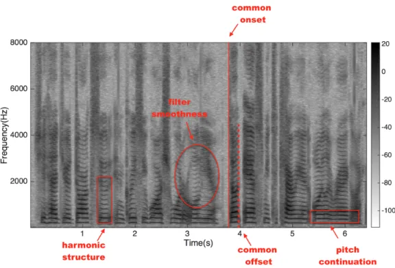
Figure 2.2: The rules formed from the observation.

2.4

Rule based source separation

Because of the physical structure, the speech contains several properties. Based on this observation, researchers proposed a serious of rule based separation(Brown and Cooke,1994;

Wang and Brown,2006;Ellis,1996b;Bregman,1994), also referred as computational auditory scene analysis(CASA). The rules can be roughly summarized as follows.

• The common onset and/or offset • Harmonic

• Pitch continuity • Vocal tract continuity • Pitch exclusiveness • Common special location • Common temporal modulation

(27)

2. Background 9

Among all rules, pitch is usually the most powerful ones. Because of the physical structure of human’s vocal track, the changing of pitch involves several muscles, which decides that the change of pitch must be continuous. Meanwhile, human can only produce one pitch at a time. Therefore, for regions that contain two or more pitches, there must be more than one sources. The harmonic and onset can also provide useful supplement since the harmonic of the sound must be the multiples of the fundamental frequency, and all the harmonic start simultaneously.

Based the those clues, in a typical CASA system, for each sample, a feature by choice is firstly calculated. Then based on hand designed rules, the TF bins are grouping into sources. Finally, a binary mask is formed based on the assignment of each TF bin, to segment the mixture. A example set of rules is cited (Shao et al.,2010) as follows:

• Low-frequency signals are grouped based on periodicity and temporal continuity. • High-frequency signals are grouped based on amplitude modulation and temporal

continuity.

• For unvoiced sounds, use a auditory segmentation and segment classification.

For CASA based system, the feature extraction step are usually the most important one, since the feature has to clearly demonstrate the grouping effect, in order to guarantee the further clustering step to generate meaningful result. Therefore, the choice of pitch tracker (Wang and Seneff,2000;Huang and Seide,2000;Lee and Ellis,2012) is essential in all CASA

systems.

Though the idea in CASA is very intuitive, it suffers from many drawbacks. The most obvious one is that it only works on speech, where there is only one pitch per time, no pitch jump and has clear continuous structure. However, for a broader perspective of audio source separation, such assumptions usually don’t hold. Another very important limitation is that all the rules are hand designed, based on the simple observation on few samples, which is clearly sub-optimum since no guaranteed that the formed rules can generalize, especially on the unvoiced sound. And since the final segmentation is based on the assignment, the best possible result is to form a oracle binary mask, which has been showed to be suboptimal in different scenarios (Wang,2005;Kjems et al.,2009). Finally, the entire system largely depend on the accuracy of pitch tracker, however, the robustness of pitch tracker can usually not guaranteed under complex acoustic condition, which leads to less robustness in separation as well.

2.5

Decomposition based source separation

In rule based system(CASA), the rules are formed based the observation on spectrogram. A natural extension is to build a system that can automatically discover the rules from data. The decomposition based model is an early attempt for this direction. The basic assumption for the decomposition based model is that the audio spectrogram has low rank structure, which can be represented with a small number of basis, as shown in (2.6).

(28)

2.5 Decomposition based source separation 10

Y =W H (2.6)

In (2.6), the spectrogramY ∈RF×T is decomposed into the matrix product of two matrix

W ∈RF×K andH ∈RK×T, whereK is the hyper-parameter, usually much smaller thanF

andT, which resulted in the low rank approximation of Y.

With different constraint, the decomposition can resulted in different specific representation. For example, the additional orthogonal constraint changes 2.6 into principle component analysis(PCA)(Jolliffe,2002), the sparsity constraint would lead to the sparse coding. In audio processing, the most popular decomposition is non-negative matrix factorization(NMF)(Lee and Seung,2001), whereW andH is constrained to be non-negative.

2.5.1

Non-negative matrix factorization

The basic formulation for NMF is shown in equation 2.7, where c is the index for each source. In2.7, each source is firstly modeled by the low rank approximation then sum to the mixture. Since both W andH are non-negative, in reconstruction of Y, there is no cancellation between sources, which models the additivity between sources in mixture, as discussed above. Y =X c WcHc Wc≥0 Hc≥0 (2.7) min W,HD(Y||W H) s.t.W ≥0, H≥0 (2.8)

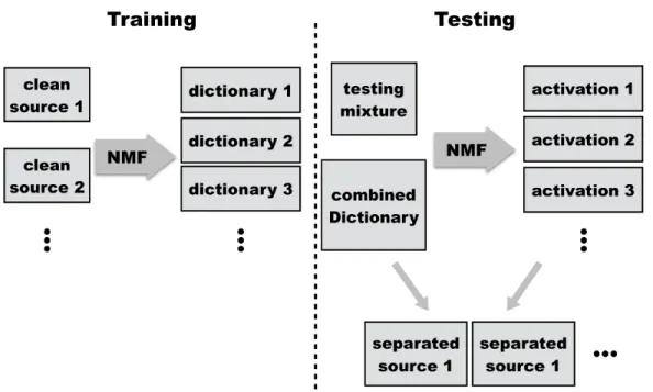
However, since the decomposition process is not convex, and the whole system is under-determinated, simply apply the decomposition on the mixture would most likely not lead to any meaningful results. In practice, the NMF based system usually has the following pipeline, as shown in fig2.3.

In training stage, the source model is usually leant by applying the decomposition on the clean sources, e.g. speech, noise, music etc. Through the decomposition, each clean source is mapped into a set of basis and activations. During the testing stage, the learnt bases for each source are fixed and only optimize the activation for each source, which makes sure that optimization is convex and a global optimum can be achieved. And finally each source is reconstructed by the pre-learnt bases and the corresponding activation. The basic NMF algorithm is given as follows. An example of NMF decomposition is given in fig2.4.

(29)

2. Background 11

Figure 2.3: Left: The training process, where a set of dictionary is learnt for each individual source. Right: The testing process, where the dictionary is fixed. After the decomposition, the reconstructed source is synthesized by each source dictionary and corresponding activation.

2.5.2

Variation of NMF

Different extensions on NMF based system were proposed based on different observation on audio signal, which is briefly summarized below.

2.5.3

Sparse NMF

Sparse NMF(Hoyer,2004;Schmidt and Olsson,2006; Virtanen,2007) further constraint the activationH to be sparse. Since the the dictionaries for each source usually shares a large amount of common pattern, e.g. pitch, the sparse constraint would increase the discrimination between sources. Moreover, since the complex pattern could usually be generating by simple patterns(for example, the white noise could be generated by the combination of all pitches), the sparsity activation would increase the robustness of the decomposition. The objective of sparse NMF is shown in2.9, where the sparsity is introduced with an additional L1 penalty on activationH.

min

W,HD(Y||W H) +αkHk1

s.t. W ≥0, H ≥0

(30)

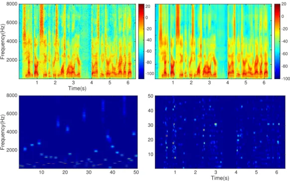
2.5 Decomposition based source separation 12 Time(s) 1 2 3 4 5 6 Frequency(Hz)₂₀₀₀ 4000 6000 8000 -100 -80 -60 -40 -20 0 20 10 20 30 40 50 Frequency(Hz)2000 4000 6000 8000 1 2 3 4 5 6 -100 -80 -60 -40 -20 0 20 Time(s) 1 2 3 4 5 6 10 20 30 40 50

Figure 2.4: Upper left: The spectrogram of clean speech. Upper right: the reconstructed speech. Bottom left: the learnt bases through the decomposi-tion. Bottom right: the learnt activadecomposi-tion.

2.5.4

Convolutional NMF

In Convolutional NMF(Behnke, 2003; Bello, 2010; Chen et al., 2014), the spectrogram is decomposed into the convolution between the basis and activation, rather than the matrix multiplication, as shown in eqn. 2.10,Here, {W(τ)} ⊂ RF+×K, τ = 1, ..., P is a set of time-varying basis elements, where each W(τ) encodes the spectra pattern of each patch at its τth frame. H ∈_RK×T

+ is the corresponding set of non-negative convolutive activations, and

τ→

H refers the “shift” operation, which padsτ zero-columns to the left ofH and truncates its rightmostP−τ columns to maintain shape, with←

τ

H defined analogously for left-shift. Compared with NMF model, the proposed model decomposes speech as the sum of convolutions between the dictionary elements and their corresponding activations. Rather than individual speech spectra, the dictionary now consists of two-dimensional “patches” of speech, which capture the energy distribution in each frequency bin over subsequent points in time. Modeling temporal dependencies in this way prevents the speech model from erroneously capturing transient noise bursts.

(31)

2. Background 13 min W,HD(Y|| P−1 X τ=0 W(τ) τ→ H) +αkHk₁ s.t. W ≥0, H ≥0 (2.10)

2.5.5

Robust NMF

Based on the observation that the noise usually has low rank structure, but hard to predict before hand, the robust non-negative matrix factorization(RNMF) combine the the NMF with robust principle component analysis(RPCA)(Cand`es et al.,2011;De la Torre and Black,

2001), another commonly used decomposition technic(Zhang et al.,2011;Chen and Ellis,

2013). In RNMF, the spectrogram is decomposed into a dictionary reconstruction and a low rank residual, as shown in eqn2.11. RNMF is specifically designed for the problem of speech enhancement, where the low rank residual models the noise and the dictionary models the speech. In eqn2.11, an additional noiseLis incorporated in the objective function. The noise is constraint to have low rank structure, which is enforced by minimizing its nuclear norm.

min H,L,EkEk 2 F+λHkHk1+λLkLk∗+I+(H) s.t. Y =W H+L+E (2.11)

2.5.6

Limitation

The main limitations for decomposition based method lays in three aspects.

Firstly, the decomposition is linear, in other words, the spectrogram is the linear combination of basis. Such assumption is made to simplify the computation, however, it omits several very important aspect of audio, for example, the long time dependence, the modulation etc. More importantly, the representation learnt through the decomposition is “shallow”. In other words, to required number of parameter increases linearly with the data variation. Therefore, it is extremely difficult to model the audio signal in detail with reasonable model size. This limitation fundamentally prevent the decomposition model to achieve high quality separation.

Additionally, the run time complexity for the decomposition model is expensive. Most of the decomposition based models are solved through iterative method, which usually require dozens of iteration to converge, even during the testing time. Therefore it is difficult to build application for the real time application. To increase the speed, the complexity of the model has to decrease.

(32)

2.5 Decomposition based source separation 14

(33)

15

Chapter 3

Neural Network

This chapter mainly introduced several fundamental aspects about artificial neural network. Inspired from the biology observation that, though the basic nerve cells are very simple. The most common neuron is named as perceptron(Hagan et al., 1996), which has the form in 3.1. In 3.1, o is the output, ik refers different input, with corresponding weight wk

and biasb,f(·) refers a non-linear function, which convert the weighted sum into a binary decision. By combining a large amount of neurons, neural network was designed to have the ability of modeling arbitrary functions. With different architecture, the network has different properties.

o=f(X

k

ikwk+b) (3.1)

3.1

Feed forward network

The feedforward neural network was the first and simplest type of artificial neural network devised(Zhang et al.,1998;Morgan and Bourlard,1990). In this network, the information moves in only one direction, forward, from the input nodes, through the hidden nodes (if any) and to the output nodes. There are no cycles or loops in the network. Each layer of the feedforward network consists the concatenation of perceptrons, followed by a non-linear function. as shown in fig3.1. The common choices of non-linearity are sigmoid, softmax and rectifier linear function, as shown in eqn3.2.

softmax: f(xi) = exi P iexi sigmoid: f(xi) = 1 1 +e−xi ReLU: f(xi) = max(0, x) (3.2)

(34)

3.2 Recurrent network 16

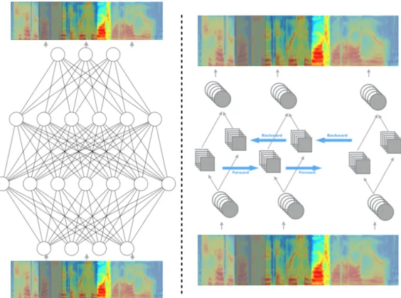
Figure 3.1: Left: An auto-encoder that consists of four layer fully connected network, with the input of the spectrogram with context window. Right: An auto-encoder of bi-directional recurrent neural network.

3.2

Recurrent network

A recurrent neural network (RNN) is a class of artificial neural network where connections between units form a directed cycle(Mikolov et al.,2010;Funahashi and Nakamura,1993). This creates an internal state of the network which allows it to exhibit dynamic temporal behavior. Unlike feedforward neural networks, RNNs can use their internal memory to process arbitrary sequences of inputs. In each layer of RNN, the relation between input and the output is given in eqn3.3. In eqn 3.3, t indexes the time step,x, handy are input, hidden states and network output,Wh and theWy are the weight with respect to the input

for hidden state and output, with corresponding biasbh andby, andU refers the weight

between consecutive hidden states, finally, the non-linearity for the hidden state and output are denoted asf(·) andg(·).

As we can see from 3.3, compared with feed forward network, the recurrent network has an additional hidden stateh, which is coupled by the additional weight U and passed through time steps. Therefore, the input from previous step could also affect the current output through this coupling, and the output at any time is the accumulation of all previous input, in other words, the network has the “memory” of the past input. This property makes the

(35)

3. Neural Network 17

RNN very appealing in audio processing since such dependence through time is one of the key feature in audio. A typical RNN is shown in fig3.1.

ht=f(Whxt+U ht−1+bh)

yt=g(Wyht+by)

(3.3)

3.2.1

Long short term memory

Although designed for the sequence processing, RNN usually suffers from the “vanishing gradient” problem, which prevent the network from capturing the long time dependency. The main reason for “vanishing gradient” comes from the coupling between time steps. In RNN, the time is captured by the multiplication of a weight matrix, i.e. Whin3.3. Then when the

eigenvalue ofWhWhT is not one, the gradient through time will explode or vanishing, a more

detailed discussion can be found in (Bengio et al.,1994).

To fix this problem, in(Hochreiter and Schmidhuber, 1997), researchers proposed a novel structure to replace the multiplicative coupling, i.e. the long short term memory(LSTM) network. The standard LSTM memory block consists of one memory cell and three gates: input gate, output gate and forget gate. The memory cell stores the state of the memory block while the gates controls the flow of activation and error, which decide the behavior of memory cell. The input gate and output gate control the flow of the activation enter and leave the memory cell. To enable the memory block to model the dependency in subsequences, the forget gate controls the memory cell to “forget” the previous activations.

We consider an LSTM memory block at nth layer with an input vectorhn_t−1 and output activationhn_t at framet (here, we omit the utterance index). Note that the input vector at the first layer corresponds to the observation vector, i.e.,h0t =yt. We first define the

concatenated vector of output activationhnt−1 at previous time framet−1 and then−1th layer output activationhn_t−1at current time frame tasmn_t _,[(h_tn−1)>,(hn_t₋₁)>]>. Then, the LSTM memory block has a memory cell (return: ct), which are obtained from the input

gate (return: it) and forget gate (return: ft):

in_t =σ(W_imn mn_t +W_icncn_t₋₁+bn_i),

f_tn=σ(W_{f m}n mn_t +W_{f c}ncn_t₋₁+bn_f),

cn_t =f_tncn_t₋₁+in_t tanh(W_cmn mn_t +bn_c),

(3.4)

whereW andbare affine transformation parameters to be estimated at the training step. , σ(·), and tanh(·) denote the element-wise product operation, sigmoid function, and hyperbolic tangent function, respectively. The memory cell and input and forget gates are calculated from the concatenated activation vectormn

t and the cell vectorcnt−1 at the previous frame. The relationship betweencn

t andcnt−1 is controlled by the forget gateftn

dynamically, which enables to retain the long-range dependency of the cell, unlike the hidden state in standard RNNs.

(36)

3.3 Objective function 18

Once we obtain cell vectorcn

t, we can calculate output gate vectoront, and finally calculate

output activationhn

t as follows:

on_t =σ(W_omn mn_t +W_ocncn_t +bn_o),

hn_t =on_t tanh(cn_t). (3.5)

A set of these equations is a basic feed-forward operation of the LSTM memory block at nth layer. At the top layer (N), output activationhNt is further calculated by the following

affine transformation:

ˆ

ht=WNhNt +b

N_. _(3.6)

This final activation ˆht would be used for the regression, classification through the softmax

operation, or masking function through the sigmoid operation.

Similar to the LSTM, Bi-directional LSTM has the same memory block as the basic unit. Instead of propagating the information in one time direction, in BLSTM layer, there are two separated propagation sequences from the both time directions. Therefore, unlike equation (3.6), the BLSTM neural network obtains the final activation ˆht by using both the final

activations from the pasthN→

t and futurehNt ←, as follows:

ˆ

ht=WN→h→t +W

N←_h←

t +b

N_. _(3.7)

This property enables the BLSTM network further explore the connection within contexts, and often lead to better performance than LSTM.

3.3

Objective function

For each neural network, a objective function is needed to measure the “correctness” of the model during the training stage. The difference between the network output and the objective can be used to update the network parameters, and lead to better accuracy. For speech enhancement, the most commonly used objective is the sum of square error(SSE), as defined in3.8. In3.8,y andxrefer the label and network output,iindexes the dimension. The euclidian distance between y andx across each dimension is summed, and used to optimize the network.

L=X

i

(yi−xi)2 (3.8)

3.4

Back propagation

The back propagation(Chauvin and Rumelhart, 1995) is a common method of training artificial neural networks and used in conjunction with an optimization method such as gradient descent. The algorithm repeats a two phase cycle, propagation and weight update.

(37)

When an input vector is presented to the network, it is propagated forward through the network, layer by layer, until it reaches the output layer. Then the network parameters are updated with gradient based optimization methods. In the back propagation process, the chain rule is used to pass the gradient backward through layer, as shown in eqn3.9

L=f(x) ∂L ∂x = ∂L ∂f ∂f ∂x (3.9)

3.5

Regularization

Due to their tendency to overfit, some form of regularization is typically necessary to ensure that the optimized neural network’s variance is not too high. A common regularizer which is used in many machine learning models is to include in the loss function a penalty on the norm of the model’s parameters. In neural networks, adding the L2 _penalty_λP

iθ

2

i

whereλis a hyperparameter andθi are the model’s parameters (e.g. individual entries of

the weight matrices and bias vectors) is referred to as “weight decay” (Hanson and Pratt,

1989). This can prevent the weight matrix of a given layer from focusing too heavily (via a very large weight value) on a single unit of its input. A related term isλP

i|θi|which

effectively encourages parameter values to be zero (Bengio,2012).

A completely different regularization method which has recently proven popular in neural networks is “dropout” (Hinton et al., 2012b). In dropout, at each training iteration each unit of each layer is randomly set to zero with probabilityp. After training, the weights in each layer are scaled by 1/p. Dropout intends to prevent the units of a given layer from being too heavily correlated with one another by randomly artificially removing connections. More simply, it provides a source of noise which prevents memorization of correspondences in the training set and has been shown empirically and theoretically (Wager et al., 2013) to be an effective regularizer.

In practice, the technique of “early stopping” is almost always used to avoid overfitting in neural network models (Prechelt,2012). To utilize early stopping, during training the performance on a held-out “validation set” (over which the parameters of the network are not optimized by gradient descent) is computed. Overfitting is indicated by performance degrading on the validation set, which simulates real-world performance. As a result, early stopping effectively prevents overfitting by simply stopping training once the performance begins to degrade. The measure of performance and criteria for stopping my vary widely from task to task (and practitioner to practitioner) but the straightforwardness and effectiveness of this approach has led it to be nearly universally applied.

(38)

3.6 Neural network in audio processing 20

3.6

Neural network in audio processing

3.6.1

Context window

The context window is one the most commonly used trick in the audio processing(Hermansky et al., 2000; Hinton et al., 2012a). Context window refers the a moving window on the input, which extents the current input to a combination of feature within a time range. The intuition behind the context window is straightforward. In English, syllable is the the shortest meaningful acoustic unit, which usually has length around 100ms, while in most speech processing application, the spectrogram frame rate is 10ms. Therefore if viewed individually, each frame in spectrogram often contain limited information and large amount of randomness, which cause difficulties for the neural network to generalize. Adding the context window could form more robust feature, thus simplify the learning process. This trick has been shown to be very effective in applications such as automatic speech recognition, speech enhancement, machine translation etc.

3.6.2

Noisy auto-encoder

A typical auto-encoder network(Deng et al.,2010;Sainath et al.,2012;Lange and Riedmiller,

2010) is shown in fig 3.2. It consists of two parts, an encoder and a decoder. With the encoder, the network first embeds the input to a fixed dimension “code”, which usually has fewer dimension than the input. Then another set of parameter, the decoder, is used to convert the embedded representation back to the input. The whole system maps the input to itself, thus called “auto-encoder”.

Auto-encoder is an important model in neural network for two reasons. Firstly, the auto-encoder maps the input to a lower dimension representation, which is invertible. In other words, it can discover a more compact representation for the data, and remove the unnecessary variances. In other words, it can have a better generalization of the data, which is essential for data processing. More importantly, since the auto-encoder learns a mapping to itself, it doesn’t require additional label to generate the gradient. Therefore, the data amount is always sufficient for auto-encoder network. Because of these two properties, the auto-encoder is usually used to initialize the network.

In practice, to improve the robustness and prevent overfit of the auto-encoder, a random noise is usually added into the input of the network, which converts the system to “noisy auto-encoder”. Experiments showed that the noisy auto encoder can learn a significantly more robust embedding of the input(Bengio et al., 2013;Rifai et al.,2011;Vincent et al.,

2010).

The noisy auto-encoder learns a transformation that can convert the noisy input to its clean version, which perfectly match the requirement for speech enhancement, where the task is to remove the noise from the noisy speech. Thus most of the neural network based speech enhancement system uses the auto-encoder based architecture(Xu et al.,2014; Narayanan and Wang,2013b). The neural network based speech enhancement system is introduced in chapter 4.

(39)

Figure 3.2: The input is firstly combined with additional noise and pass through the encoder to form the lower dimensional embedding. Then the embedding is used to generate the input through the decoder.

(40)

3.6 Neural network in audio processing 22

(41)

23

Chapter 4

Neural Network based speech

enhancement

As an universal function approximater, neural network has been successfully applied in different applications. In the problem of speech enhancement, the neural network also achieved significant performance improvement, when compared with traditional models introduced in chapter 2.

As discussed in last chapter, most of the speech enhancement system use auto-encoder architecture. Among them, two branches are most commonly adopted, the feature mapping network and mask learning network.

4.1

Feature mapping

The feature mapping network is straightforward. The network takes the noisy spectrogram as inputY, and targets at the clean spectrogramX, with the objective function shown in 4.1. In4.1, Φ(·) refers the non-linear transformation of neural network, andDrefers the distance between the output and the reference. Usually euclidian distance is chosen. The feature mapping network is simple but effective. The feature mapping network achieved significant performance improvement in comparison to the traditional models.

L=D(X||Φ(Y)) (4.1)

However, the feature mapping network also suffers from several drawbacks. The most obvious one is the unbounded dynamic range. Since the network directly output the clean spectrogram, which is unbounded, the output dynamic range has to be large enough to cover all possible volumes. Such procedure will largely increase the redundancy for the learning task. For example, for the same utterance with different amplitude, the feature mapping network need to generate completely different result, which will make the network more difficult to converge.

(42)

4.2 Mask learning 24

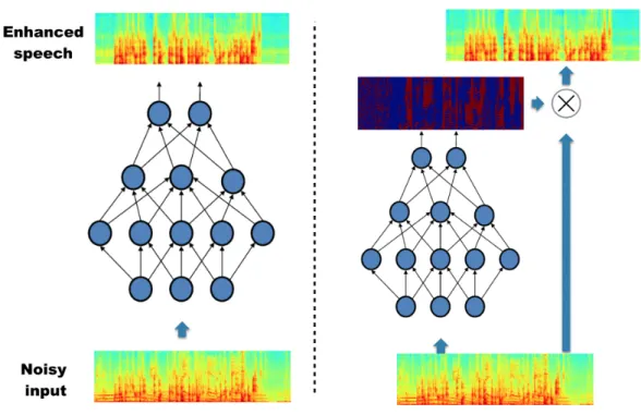
Figure 4.1: Left: the feature mapping architecture. Right: the mask learning architecture

4.2

Mask learning

Another commonly used architecture is the mask learning network. Different with the feature mapping network that directly output the clean spectrogram, the mask learning network output a mask, which can be applied back to the noisy signal and mask out the noise, as shown in figure4.1. A typical objective function is shown in6.2, whereY andX refer the input feature and clean reference accordingly. Φ(·) refers the non-linear function learnt by the neural network andD(·) refers the distance measure, which is usually euclidean distance.

L=D(X||Φ(Y)) (4.2)

There are two ways to learn the mask. The first one is called mask approximation (MA) which directly minimizes the distance between the learned mask and the target mask (Narayanan and Wang,2013a,2014b,a;Wang et al.,2014a). The second is called signal approximation (SA) which minimizes the distance between the target signal and the signal constructed by applying the estimated mask to the distorted signal (Weninger et al.,2014b;Erdogan et al.,

2015b).

Since the mask is bounded(e.g. the mask usually has value in [0,1]), the mask learning network has the fixed dynamic range. Therefore it is easier for the the mask learning network to generalize different noises, conditions. Moreover, as shown in fig4.1, during the separation,

(43)

4. Neural Network based speech enhancement 25

since the mixture is re-introduced to the computation, the network only needs to filter out the noisy part. Compared with the feature mapping network, where the system need to both remove the noise and remember the clean reference, the learning task for mask based system is easier, and thus usually leads to better performance, as reported in (Narayanan and Wang,

2013b;Wang and Wang,2013;Healy et al., 2013)

We choose signal approximation based mask learning in this study. It is shown in (Weninger et al.,2014b) that SA is better than MA as its final target is directly related with the source signal. The objective of SA based mask learning for speech enhancement is:

L=kX−Φ(Y)Mk2₂, (4.3)

where X and M are clean speech and noisy speech in the mask learningoutput feature domain;Y is the noisy speech in the mask learning input feature domain; Φ(·) is the mask estimation function learnt from neural networks. Φ(Y)∈[0,1] is the learnt soft mask. The effectiveness of the auto-encoder based speech enhancement has been shown in different works(), one of the most representative one is on the 2nd CHiME speech separation and recognition challenge, where different speech enhancement methods were evaluated under different frame work.

The noisy data in ChiME challenge was constructed from the Wall Street Journal dataset. The clean 16kHz WSJ data was firstly convolved with the room impulse response to model the reverberation. Then the reverberated speech was mixed with the recorded background noise the at 6 different SNRs from−6dBto 9dB. The training set contains 7138 utterances from 83 speakers, totaling 14.5 hours. The development set contains 4.5 hours data, which consists of 2460 utterances from 10 speakers that are disjoint with the training set. The test set consists of 1980 utterance from 8 speakers, 4 hours in total.

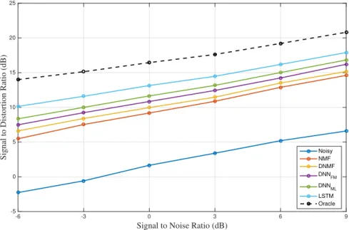
Four models were evaluated(Le Roux et al., 2015a; Weninger et al., 2015; Chen et al.,

2015), including two mask learning based models using feedforward network(DNN) and bi-directional long short term memory(BLSTM) network. The DNN consists of three layers, each layer had 1024 nodes, with hyperbolic tangent function for non-lineariry, followed by an output layer, which was a feedforward layer of 100 nodes with sigmoid function. The input feature for the DNN were the 100 dimension log mel-filterbank, withT = 9 context window. The spectrogram was calculated using 25 ms window size and 10 ms window shift. For the BLSTM network, each BLSTM layer had 300 forward LSTM cell and 300 backward cell. Similar to DNN network, an output layer was added after the BLSTM network to generate the mask. No context window is used for the BLSTM network. All the input feature was normalized with zero mean and unit variance.

The discriminate non-negative matrix factoration(DNMF) and plain NMF were included as the baseline. The spectrogram was calculated using 25 ms window size and 10 ms window shift. With 9 consecutive frames, the concatenated spectrogram was used as feature. The dictionary size was set to 1000. The performance of NMF based models on the same data was cited from (Le Roux et al.,2015a). And the full evaluation is shown in fig4.2.

In fig4.2, the neural network based methods outperformed the NMF based model by a large margin on every condition. As discussed in previous chapter, the LSTM network outperforms the DNN, because of the sequence modeling. The dash line showed in fig4.2refers the result

(44)

4.2 Mask learning 26

Signal to Noise Ratio (dB)

-6 -3 0 3 6 9

Signal to Distortion Ratio (dB)

-5 0 5 10 15 20 25 Noisy NMF DNMF DNN FM DNN ML LSTM Oracle

Figure 4.2: The CHiME 2 speech enhancement evaluation

using oracle ratio mask. Note that the LSTM is only 3.34Db on average lower than the oracle, showing its effectiveness.

(45)

4.3

Improving the mask learning network

The mask learning network showed significant performance in contrast to previous models. However, there are several limitations.

4.3.1

Scale Mismatch Problem

The main limitation for mask learning network lies in the assumption that the scale of the masked signal is the same as the clean target. Using masks as the training target is supposed to remove only the noise distortion. If the distorted signal is also impacted by the channel distortion, an additional feature mapping function has to be learned to remove the channel distortion in the enhanced speech feature estimated via mask learning. This problem is even more severe in the far-talking scenarios. With a few exceptions for some synthetic data, this assumption is usually not applicable for most real recorded parallel data due to the varied sound source location and the differences in microphones. We refer this as “scale mismatch problem”.

When the mixture (M), clean speech (X), and the noise (N) are strictly additive, i.e. M =X+N, the clean speech can be perfectly recovered from the ideal mask (i.e. _XX₊_N) learned from the neural network. Nevertheless, the same scale assumption in mask learning is only true on some synthetic data.

For real recorded data, due to the sound source location and microphone differences between far-talk and far-talk channels, their recordings can vary significantly both in scale and spectrum. This is the “scale mismatch problem”.

In real parallel recording, mixture from a far-talk microphone (M) and clean speech (X) can be represented as

M =f(g(X) +N), (4.4)

wheref(·) is the non-linear transformation introduced by the channel mismatch;g(·) repre-sents the spectral difference between the two recordings.

The masking process Φ (Y)M would fail to recover the clean speech due to the cascaded non-linearities, even with the ideal mask.

4.3.2

Mask Learning with Restoration Layer

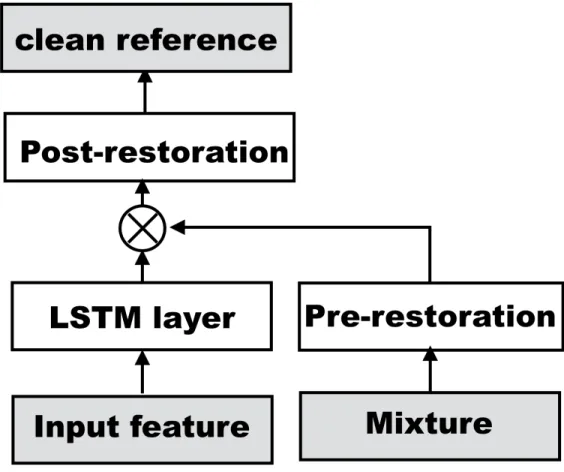
We propose to extend the mask learning with two types of restoration layers before or after the mask to address the scale mismatch problem, namely pre- and post-restoration layers. In the mask learning with pre-restoration layers, the noisy speech first passes through fully connected neural network layers with rectifier linear unit activation (ReLU); then combines with the learnt [0,1] mask φ(Y). Since ReLU is unbounded, the pre-restoration layer is designed to learn the scale mismatch between the mixture and the reference. Alternatively,

(46)

4.3 Improving the mask learning network 28

in the mask learning with post-restoration layers, the scale restoration happens after the mask learning through fully-connected neural network layers.

Figure4.3depicts the architecture of the extended mask learning with pre- or post-restoration layers. Both pre- and post- restoration layers are designed to fix the scale mismatch problem in mask learning. The key differences lie in that post-restoration layers, as the last step in speech enhancement, have the potential to fix the additional scale-related spectral patterns re-introduced during masking.

Figure 4.3: Input feature, mixture and clean reference blocks correspond Y, M andX in Equation 5.1, and the remaining white blocks are neural network parameters(Φ(·) in Equation5.1)

With this extension, the mask learning based speech enhancement can be applied to a wide range of real world scenario. We will present results on the mask learning with restoration layers on CHiME3 task in Section6.5.

(47)

4.4

Residual Learning Feature Mapping

In this section, we introduce applying the residue learning architecture to speech enhancement.

4.4.1

Background of Residual Network

Deep residual learning makes use of short cut connections between neural network layers for fast convergence. It was first proposed in (He et al.,2015) for image recognition. Lately its efficacy was also confirmed in large vocabulary speech recognition (Xiong et al.,2016a). In residue network, neural network layers are explicitly reformulated to learn residual functions with respect to the layer inputs. The short-cut connection in deep residue learning effectively addresses gradient vanishing/exploding problem in very deep neural network. Thus it is generally believed that very deep neural networks with residue connections is easier to optimize. The residue learning helps to maintain consistently improved accuracy performance in increasingly deeper and more complicated neural network.

Most previous work in applying residue learning focuses on improving network optimization for very deep network.

4.4.2

Residual Learning for Speech Enhancement

Unlike solving gradient vanishing/exploding problems and ease of training of very deep net-work, the motivation behind our work in applying the residue learning in speech enhancement has straightforward physical meaning in signal reconstruction.

Multiplication in linear scale corresponds to summation when performed in logarithm scale. In a feature mapping network, when the input feature is in logarithmic scale, e.g. log-spectrogram, log-mel-filterbank, etc., adding the additive residual connection between layers is equivalent to perform the masking learning.

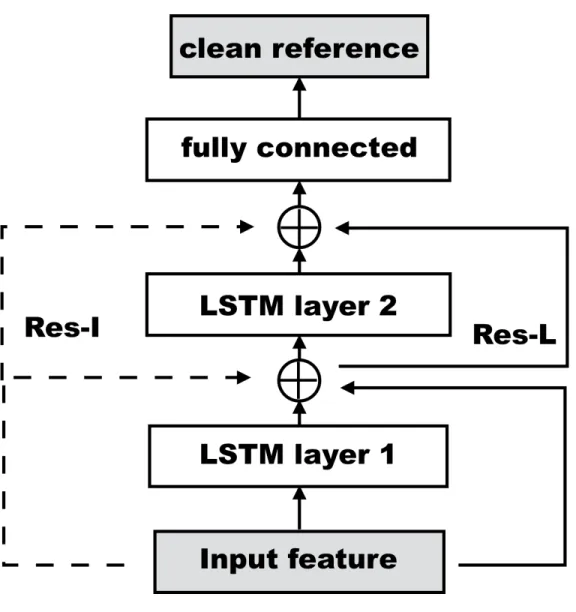
Based on this observation, we propose a residual learning based architecture for enhancement. Two types of residual connection are proposed: input residual connection and layer-wise residual connection. In the input residual connection, the shortcut connection between input and the output of each layer is incorporated in the network. In layer-wise residual connection, the shortcut is added between the output of each layer and its previous layer.

Figure4.4presents the architecture of residual learning based speech enhancement usinginput

residue connection and/orlayer-wise residue connection. Introducing residue connections in feature mapping network allows us to benefit from both feature mapping and mask learning. This architecture alternates between the feature mapping and mask learning cross different neural network layers. Therefore, it can potentially outperforms speech enhancement with the mask or the feature mapping only.

(48)

4.5 Experiment 30

Figure 4.4: Architecture of the residue-learning based speech enhancement model

Architecture of the residue-learning based speech enhancement model

4.5

Experiment

In this section, we present our speech enhancement experimental results on the CHiME3 task.

(49)

4.5.1

CHiME 3 and ASR Back-End

CHiME 3 (Barker et al.,2015a) data is recorded using a 6-channel microphone array mounted on a tablet. The training data consists of 1600 real noisy utterances and 7138 simulated utterances. The real data is recorded in different live environments. The simulated data is obtained by mixing clean utterances into different background recordings. For both real and simulated data, four environments are selected: cafi (CAF), street (STR), public transport (BUS), and pedestrian area (PED).

We train a fully connected deep neural network (DNN) on close-talk clean speech. The DNN has 7-hidden layers, each with 2048 hidden units. The input consists of a 2640-dim feature vector formed by 80-dim LFB feature and its accelerating feature components with a context window of 11 frames (80*3*11=2640). The output layer has 3012 senone states. We adopt the RBM pre-training before the fine-tuning of the full network using the cross-entropy criteria. We use WSJ 5K word 3-gram LM for decoding throughout this paper.

The model is then evaluated on the multi-channel enhanced speech audio provided by the CHiME 3 speech challenge (Barker et al.,2015a) and the single-channel far-field noisy speech. The proposed single-channel speech enhancement models are applied as a plug-in module before decoding.

4.5.2

Extended Mask Learning with Restoration Layers

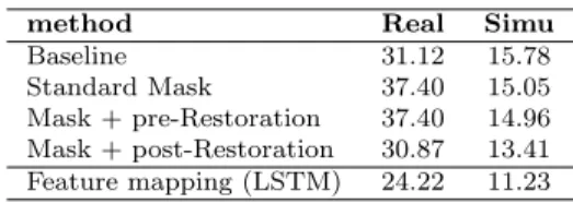
We use a two-layer 300-cell LSTM for masking learning and a feed-forward projection layer with sigmoid activation injected before or after the mask learning layers for scale restoration. The input is 100-dimension log mel-filterbank, calculated with 25ms window and 10ms hop. The setup is similar to a previous state-of-art mask learning system(Barker et al.,2015b). We compare the plain mask learning with the extended mask learning with pre- or post-restoration layers. As shown in Table 4.1, without scale restoration, the mask learning completely fails on both real and simulated data. This confirms the scale mismatch problem described earlier. After introducing scale restoration layers, both pre-restoration and post-restoration layer improves the mask learning result. In particular, we found that the post-restoration outperforms the pre-restoration. This is likely due to the fact that the post-restoration layers have more information from bottom layers and can be better optimized globally.

In addition, we compare the mask learning based approach with the feature mapping approach. Here the feature mapping is conducted in the acoustic model feature domain. The input is the 240-dim log mel-filterbank formed by 80-dim log mel-filterbank with double delta, as described in Section 4.5.1; the output is the 80-dim log mel-filterbank feature. A similar two-layer 300-cell LSTM is used. It can be seen from Table4.1that feature mapping learning in the acoustic model feature domain significantly outperforms the mask-learning based approach, even with injected restoration layers. We believe that this is due to the extra noise introduced during the signal conversion in the mask learning based speech enhancement. Lastly, we compare three feature mapping networks using DNN, LSTM, or bLSTM. All three models have comparable number of model parameters. The DNN has four hidden layers

(50)