Bayesian Structured Representation Learning

(1)

UC San Diego

UC San Diego Electronic Theses and Dissertations

Title

Bayesian Structured Representation Learning Permalink

https://escholarship.org/uc/item/8hp480fc Author

Vikram, Sharad Mandyam Publication Date 2019

(2)

UNIVERSITY OF CALIFORNIA SAN DIEGO

Bayesian Structured Representation Learning

A dissertation submitted in partial satisfaction of the requirements for the degree

Doctor of Philosophy in Computer Science by Sharad Vikram Committee in charge:

Professor Sanjoy Dasgupta, Chair Professor Gary Cottrell

Professor Julian McAuley Professor Lawrence Saul Professor Zhuowen Tu

(3)

Copyright Sharad Vikram, 2019

(4)

The dissertation of Sharad Vikram is approved, and it is ac-ceptable in quality and form for publication on microfilm and electronically:

Chair

University of California San Diego

(5)

Foundations

3

Chapter 2 Bayesian Structure Learning . . . 4

2.1 What is structure learning? . . . 4

2.1.1 Linear dynamical system . . . 5

2.1.2 Hierarchical clustering . . . 6

2.2 Bayesian structure learning . . . 7

2.2.1 Bayesian linear dynamical system . . . 10

Chapter 3 Bayesian Nonparametric Hierarchical Clustering . . . 12

3.1 Background . . . 13

3.1.1 Traditional hierarchical clustering . . . 13

3.2 The generative process . . . 16

3.2.1 Tree priors . . . 17

3.2.2 Generalizations of coalescent and diffusion models . . 24

3.2.3 Other priors . . . 26

3.2.4 Tree likelihood models . . . 29

3.2.5 Inference . . . 30

Chapter 4 Interactive Bayesian Hierarchical Clustering . . . 33

4.1 Adding interaction . . . 37

4.1.1 Triplets . . . 38

4.1.2 Finding a tree consistent with constraints . . . 39

(6)

4.1.4 Intelligent subset queries . . . 44

4.2 Experiments . . . 45

4.3 Future Work . . . 48

Chapter 5 Representation Learning . . . 49

5.1 PCA and autoencoding . . . 50

5.2 The variational autoencoder . . . 50

5.2.1 Variational inference . . . 52

5.2.2 Inference in the VAE . . . 54

5.2.3 Extensions and applications of the VAE . . . 56

II

Combining Structure and Representation Learning

58

Chapter 6 Introduction . . . 59

Chapter 7 Neural Variational Message Passing . . . 62

7.0.1 Related Work . . . 64

7.1.1 Exponential families and conjugacy . . . 65

7.1.2 Mean field variational inference . . . 67

7.1.3 Variational message passing . . . 69

7.2 Neural variational message passing . . . 70

7.2.1 Learning recognition network weights . . . 73

7.2.2 Lower-bounding the ELBO . . . 73

7.2.3 Extensions to NVMP . . . 74

7.3 Examples and experiments . . . 74

7.3.1 Bayesian linear regression with a sparse prior . . . 75

7.3.2 Bayesian logistic regression . . . 76

7.3.3 SVAE-GMM . . . 77

7.3.4 Nonlinear dynamical system . . . 77

7.4 Discussion . . . 78

Chapter 8 Deep Bayesian Hierarchical Clustering . . . 79

8.1.1 Bayesian priors for hierarchical clustering . . . 81

8.1.2 Variational autoencoder . . . 84

8.2 The TMC-VAE . . . 85

8.3 LORACs prior for VAEs . . . 87

8.4 Related work . . . 90

8.5 Results . . . 90

8.5.1 Qualitative results . . . 91

(7)

Chapter 9 Structured Representations for Reinforcement Learning . . . 100

9.1 Introduction . . . 100

9.2 Preliminaries . . . 102

9.3 Learning and Modeling the Latent Space . . . 104

9.3.1 The Deep Bayesian LQS Model . . . 106

9.3.2 Joint Model and Representation Learning . . . 107

9.4 Inference and RL in the Latent Space . . . 111

9.5 The SOLAR Algorithm . . . 112

9.5.1 Transferring Representations and Models . . . 113

9.5.2 Learning from Sparse Rewards . . . 114

9.6 Related Work . . . 115

9.7 Experiments . . . 116

9.7.1 Experimental Tasks . . . 117

9.7.2 Comparisons to Prior Work . . . 119

9.7.3 Analysis of Real Robot Results . . . 122

Appendix A Exponential family distributions . . . 124

A.1 Categorical distribution . . . 124

A.1.1 Exponential family parametrization . . . 125

A.2 Dirichlet distribution . . . 125

A.3 Gaussian distribution . . . 126

A.4 Inverse-Wishart (IW) distribution . . . 126

A.5 Normal-inverse-Wishart (NIW) distribution . . . 127

A.6 Matrix normal (MN) distribution . . . 128

A.7 Matrix normal inverse-Wishart (MNIW) distribution . . . 129

Appendix B Supplementary material for Chapter 4 . . . 131

B.1 Proof Details . . . 131

(8)

Appendix C Supplementary material for Chapter 7 . . . 135

C.1 Proof of ELBO lower bound . . . 135

C.2 Extension: stochastic variational inference . . . 136

C.3 Extension: amortized inference . . . 137

Appendix D Supplementary material for Chapter 8 . . . 139

D.1 Additional visualizations . . . 139

D.2 Empirical results . . . 139

D.3 Algorithm details . . . 139

D.3.1 Stick breaking process . . . 139

D.3.2 Belief propagation in TMCs . . . 142

D.3.3 Variational inference for the LORACs prior . . . 147

D.4 Details of experiments . . . 150

D.4.1 Baseline details . . . 151

Appendix E Supplementary material for Chapter 9 . . . 155

E.1 Policy Learning Details . . . 155

E.2 Parameterizing the Cost Model . . . 156

E.3 The SVAE Algorithm . . . 157

E.4 Fitting the Local Dynamics Model . . . 158

E.5 Experiment Setup . . . 159

E.6 Implementation of Comparisons . . . 162

E.7 Additional Experiments . . . 164

E.7.1 RCE on Fixed-Target 2D Navigation . . . 164

E.7.2 Full Learning Progress of PPO . . . 165

(9)

LIST OF FIGURES

Figure 2.1: The graphical model for a linear dynamic system . . . 6 Figure 2.2: Graphical model for hierarchical clustering . . . 7 Figure 2.3: Examples of ambiguous hierarchical structure in data. The left set

of points could plausibly be hierarchically clustered in three different ways. The right set of points has two plausible hierarchical clusterings. 8 Figure 2.4: Examples of how Bayesian structure learning could uncover ambiguity

in latent structure. In (a), all three possible clusterings are given equal probability and in (b), the two most likely clusterings split the probability. 9 Figure 2.5: The graphical model for Bayesian structure learning. Note the addition

of a prior distribution over the structure. . . 10 Figure 2.6: The graphical model for a Bayesian linear dynamical system. Note the

addition of a prior over the dynamics parameters. . . 10 Figure 3.1: Hierarchies over human tumor data produced by agglomerative

clus-tering with three different linkage criteria. Image from Hastie et al. (2009). . . 15 Figure 3.2: The graphical model used in Bayesian hierarchical clustering. τ is a

tree, sampled from a tree prior distribution. . . 16 Figure 3.3: A sample from Kingman’s coalescent. zis the common ancestor for

datax_1:4. Eachy_C represents the common ancestor for data subsetC. The axis represents time, and eachδirepresents elapsed time.π(t)is

the genealogy function. Image from Teh et al. (2008). . . 19 Figure 3.4: For the balanced tree on the left, there are two possible orderings

in which clusters were merged, whereas there is only one possible ordering for the unbalanced tree on the right. Image taken from Boyles and Welling (2012). . . 20 Figure 3.5: On the left is a sample Dirichlet diffusion tree. Black dots correspond

to nodes in the tree. The image is taken from Vikram and Dasgupta (2016). On the right is a sample from a Pitman-Yor diffusion tree with 4 points. The image is taken from Knowles and Ghahramani (2015). 23 Figure 3.6: A graph visualization of the relationships between various tree priors.

Directed arrows represent specific cases of a distribution or model. . . 26 Figure 3.7: A visualization of a sampled from a nested Chinese restaurant process

(NCRP). Only three levels for 5 customers are shown. Image from Blei et al. (2010). . . 27 Figure 3.8: Visualization of a subtree-prune and regraft move for a tree with four

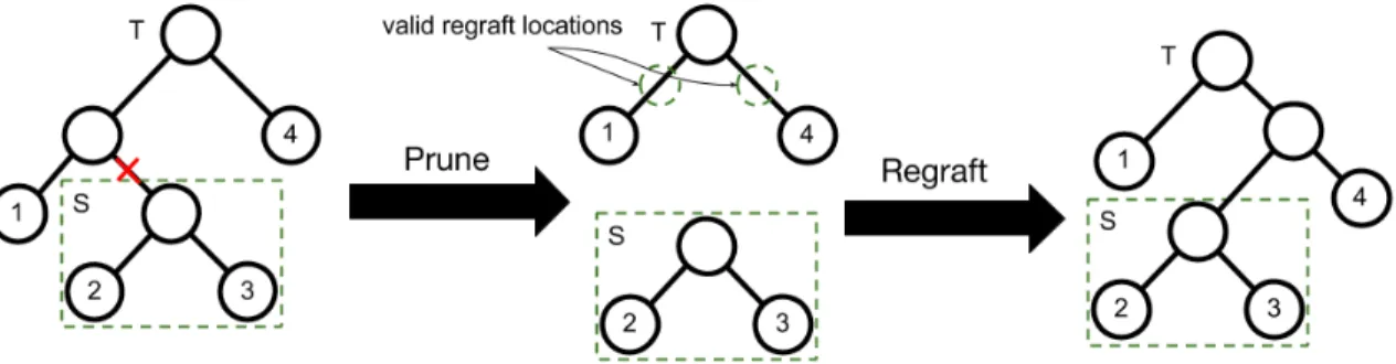
leaves. Image from Vikram and Dasgupta (2016). . . 31 Figure 4.1: Target treeT∗(left) and a refinement of it. . . 38

(10)

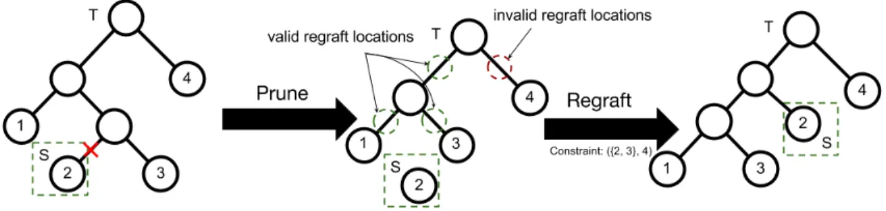
Figure 4.2: Visualized is a constrained-SPR move. Pruning is identical but a regraft location is selected from the valid regraft locations limited by triplets.

In this image, we are constrained by the sole triplet({2,3},4). . . . 40

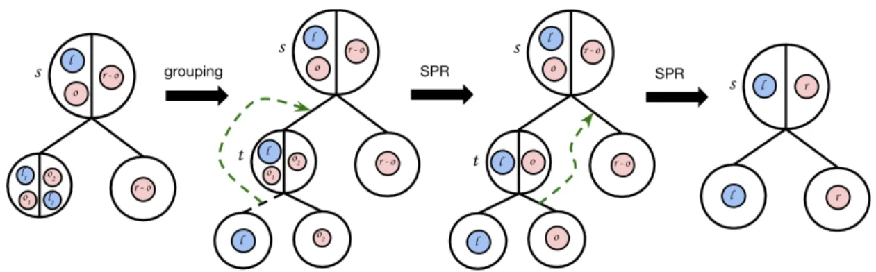
Figure 4.3: The process of convertingsinto canonical form. We first group nodes froml into their own isolated subtree, then perform two constrained-SPR moves to putsinto canonical form. . . 42

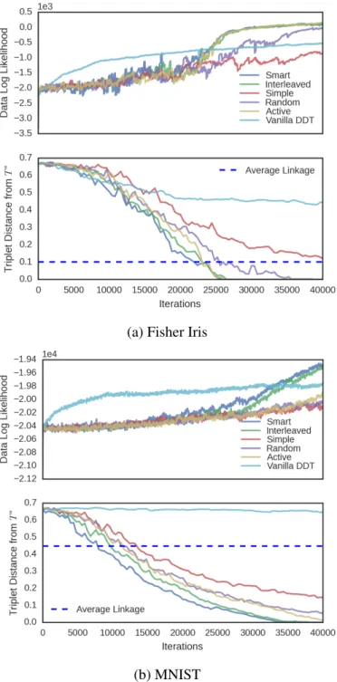
Figure 4.4: The average of four runs of constrained-SPR samplers for the Fisher Iris dataset and the MNIST dataset, using 5 different querying schemes. A query was made every 100 iterations. . . 46

Figure 5.1: The graphical model for representation learning . . . 55

Figure 6.1: The graphical model for Bayesian structured representation learning . 60 Figure 7.1: The messages that need to be computed in order to update node zn in variational message passing. Specifically, we require messages computed over the Markov blanket ofz_n. . . 68

Figure 7.2: Five nonconjugate models in which NVMP messages can be used for approximate inference. . . 75

Figure 7.3: A learned “circular” dynamics system using NVMP. . . 78

Figure 8.1: Independent samples from a time-marginalized coalescent (TMC) prior and two-dimensional Gaussian random walk likelihood model (10 and 300 leaves respectively). Contours in the plots correspond to posterior predictive densityr(zN+1|x1:N,τ). . . 81

Figure 8.2: Graphical models and variational approximations for TMC models described in the paper . . . 87

Figure 8.3: Learned inducing points for a LORACs(200) prior on MNIST. . . 91

Figure 8.4: An example learned subtree from a sample of q(τ;s1:M) for each dataset. Leaves are visualized by passing inducing points throught the decoder. . . 92

Figure 8.5: The evolution of a CelebA over a subset of inducing points. We create this visualization by taking slices of the tree at particular times and looking at the latent distribution at each of the sliced branches. . . 93

Figure 8.6: Conditional samples from subtrees. . . 94

Figure 8.7: Samples from subtrees of CelebA. . . 95

Figure 8.8: Few-shot classification results . . . 95

Figure 8.9: TSNE visualizations of the latent space of the MNIST test set with different priors, color-coded according to class. LORACs prior appears to learn a space with more separated, concentrated clusters. . . 97

Figure 9.1: Examples of our method’s success at solving real world robotics tasks within one to two hours of interaction time . . . 101

(11)

Figure 9.2: A high-level schematic of our method. We discuss the details of the model and inference procedure in section 9.3 and section 9.4. We then

explain our algorithm in section 9.5. . . 105

Figure 9.3: The generative model used by SOLAR . . . 110

Figure 9.4: Illustrations of the environment we evaluate our algorithm on . . . . 117

Figure 9.5: Results of SOLAR on simulated tasks . . . 119

Figure 9.6: Results of SOLAR on real robotics tasks . . . 121

Figure 9.7: Left: our method learns a policy with better final performance using slightly less data compared to deep visual foresight. Right: visualizing example end states from rolling out our policy after 200 (top), 230 (middle) and 260 (bottom) trajectories. . . 121

Figure B.1: The process of grouping the data in uthat belong tol into their own pure subtree. uis the lowest node oft (see Figure 4.3) that has data fromlin both of its children. . . 133

Figure B.2: The process of convertingsinto canonical form. We first group nodes fromlinto their own pure subtree, then perform two constrained-SPR moves to putsinto canonical form. . . 134

Figure B.3: The average of four runs of constrained-SPR samplers for the Zoo dataset and the 20 Newsgroups dataset, using 5 different querying schemes. A query was made every 100 iterations. . . 134

Figure D.1: TSNE visualizations of the latent space of the MNIST test set with various prior distributions, color-coded according to class. . . 142

Figure D.2: A TSNE visualization of the latent space for the TMC(200) model with inducing points and one sample fromq(τ;s1:M)plotted. Internal nodes are visualized by computing their expected posterior values, and branches are plotted in 2-d space. . . 143

Figure D.3: MNIST VampPrior learned pseudo-inputs. . . 144

Figure D.4: MNIST VampPrior reconstructed pseudo-inputs obtained by determin-istically encoding and decoding each pseudo-input. . . 144

Figure D.5: Omniglot learned inducing points. . . 152

Figure D.6: CelebA learned inducing points. . . 153

Figure D.7: Averaged precision-recall curves over test datasets. . . 154

Figure E.1: On 2D navigation with the goal fixed to the bottom right, RCE is able to successfully learning a policy for navigating to the goal. . . 164

(12)

LIST OF TABLES

Table 8.1: Averaged precision-recall AUC on MNIST/Omniglot test datasets . . . 98

Table 8.2: MNIST/Omniglot test log-likelihoods . . . 98

Table D.1: MNIST few-shot classification results. . . 140

Table D.2: Omniglot few-shot classification results. . . 141

Table D.3: MNIST few-shot classification with labeled inducing points. . . 142

Table D.4: Network architectures for MNIST and Omniglot . . . 150

(13)

ACKNOWLEDGEMENTS

I am grateful for my advisor, Sanjoy Dasgupta, not only for supporting and advising me, but also for helping me find opportunities to work on projects I could have only dreamed about before.

I would like to thank my collaborators, Pieter Abbeel, Matthew Hoffman, Matthew Johnson, Sergey Levine, Laura Smith, and Marvin Zhang, who have all been sources of inspiration and insight throughout graduate school.

I am grateful to all my UCSD colleagues and friends, who have provided countless hours of interesting discussion and entertaining conversation over the years, including Julaiti Alafate, Chris Donahue, Wang-Cheng Kang, Zachary Lipton, Stefanos Poulis, and Christopher Tosh.

Finally, I would like to thank my parents, my brother, my grandparents, and Iris, all of whose love and support throughout graduate school have been invaluable to my success. To my late grandfather, M.K. Sridhar, thank you for inspiring and teaching me with your passion for computer science and technology.

Chapter 4, in full, is a reprint of material as it appears in “Interactive Bayesian Hierarchical Clustering”. S. Vikram and S. Dasgupta. In International Conference on Machine Learning 2016. The dissertation author was the primary investigator.

Chapter 7, in full, contains material that is currently being prepared for submission for publication. S. Vikram. The dissertation author is the primary investigator.

Chapter 8, in full, is a reprint of the as it appears in “The LORACs Prior for VAEs: Letting the Trees Speak for the Data”. S.Vikram, M. Hoffman, and M. Johnson. In International Conference on Artificial Intelligence and Statistics 2019. The dissertation author was the primary investigator.

(14)

Representations for Model-Based Reinforcement Learning”. M. Zhang*, S. Vikram*, L. Smith, P. Abbeel, M. Johnson, and S. Levine. In International Conference on Machine Learning 2019. The dissertation author was one of two primary investigators.

(15)

VITA

2014 B. S. in Electrical Engineering and Computer Science, University of California, Berkeley

(16)

ABSTRACT OF THE DISSERTATION

Bayesian Structured Representation Learning

by

Sharad Vikram

Doctor of Philosophy in Computer Science

University of California San Diego, 2019

Professor Sanjoy Dasgupta, Chair

Bayesian methods offer the flexibility to both model uncertainty and incorporate domain knowledge into the modeling process. Deep generative modeling and Bayesian deep learning methods, such as the variational autoencoder (VAE), have expanded the scope of Bayesian methods, enabling them to scale to large, high-dimensional datasets. Incorporating prior knowledge or domain expertise into deep generative modeling is still a challenge, often resulting in models where Bayesian inference is prohibitively slow or even intractable. In this thesis, I first motivate using structured priors, presenting a contribution in the space of interactive structure learning. I then define Bayesian structured representation

(17)

learning (BSRL) models, which combine structured priors with the VAE, and present foundational work along with applications of BSRL models.

(18)

Chapter 1

Introduction

In machine learning problem settings, we are often presented with data but addi-tionally have information about how the data was collected or generated. Furthermore, we may have knowledge or access to domain expertise that could inform a learning algorithm. Traditionally, one way of incorporating prior knowledge or domain expertise into machine learning algorithms is by formulating them as probabilistic graphical models, which offer flexible avenues for incorporating assumptions about data. Take, for example, if we are tasked with discovering clusters in a dataset, but have prior knowledge that the features of the data are disentangled or independent, we can incorporate that information into the prior distribution over cluster components.

This strategy, however, has major downsides, namely that the types of assumptions that can be incorporated into probabilistic graphical models have been historically limited to generative models in which Bayesian inference is tractable. Thus, in scenarios where the data is high-dimensional and exhibits complex structure, we are forced to make restrictive assumptions that enable tractable inference, but limit the capacity of our model.

On the other hand, neural networks have emerged as a dominant force in machine learning, thanks to their ability to scale to large datasets and their empirical success on

(19)

complex data like images and text. Incorporating prior knowledge or domain expertise into deep learning approaches has often taken the form of custom neural network layers or architectures that are tailored to the task at hand, and although these strategies have seen empirical success, they are often ad-hoc solutions and do not leverage the explicit assump-tions and modeling of uncertainty that probabilistic graphical models offer. Combining deep learning methods with probabilistic graphical models has thus been recent topic of interest with many open problems and challenges.

Much work has gone into investigating which models are tractable and how to approximate intractable ones. One of the most prominent methods to emerge in unsuper-vised learning is the variational autoencoder (VAE; Kingma and Welling, 2014; Rezende et al., 2014), which frames autoencoding as a probabilistic latent variable model. The VAE models through a generative process where latent codes are sampled from a prior distribution, and are then passed through a neural network decoder. The encoder is used for inference, approximating the posterior distribution of codes given data.

The VAE is a stepping stone for incorporating neural networks into statistical learning, but in its original form, contains very simple assumptions. The statistical learning literature, on the other hand, has explored a wide variety of models and structures for data. In this thesis, we motivate and discuss the use of Bayesian structured priors and the algorithmic challenges in incorporating them with deep generative models. The combination of a Bayesian structured prior with a VAE results in a class of models called Bayesian structured representation learning models.

In Part I, we introduce the core ideas and foundations for Bayesian structure learning and present a contribution in the space of interactive structure learning. In Part II, we motivate and discuss algorithms and models used in Bayesian structured representation learning.

(20)

Part I

(21)

Chapter 2

Bayesian Structure Learning

In this chapter we define the Bayesian structure learning problem and cover relevant technical background material.

2.1

What is structure learning?

Learning structure is a broad problem; we define it as an unsupervised learning problem wherein a user has data and a priori assumes some unobserved, orlatent, organiza-tion of the data. Example organizaorganiza-tions of the data might include a flat clustering, i.e. the data can be partitioned into someK distinct groups. A logical extension of a flat clustering organization is a mixed-membership model, where data can be organized intoK groups but each datum may belong to many groups simultaneously. In this thesis, we are particularly interested in hierarchical clustering, where data are organized into a tree structure, with data closer on the tree being logically or semantically similar. We are also interested in linear dynamical systems, wherein time-series data evolve according to a linear transition function.

(22)

class. It then recovers a plausible structure and returns it to the user. Formally, we assume a structure class T and return a candidate structureτ ∈T . Perhaps the most famous

is the K-means problem, which assumes K discrete clusters to which the data belong. The corresponding algorithm recovers a K-partition of the data. Analogously in mixed-membership modeling, latent Dirichlet allocation (LDA; Blei et al., 2003) recovers a topic model structure for text data.

We formalize structure learning probabilistically. We will later cover the Bayesian variant, but in vanilla structure learning, there exists some latent structureτ and a likelihood

functionp(x1:N|τ). Recovering a structure amounts to maximizing likelihood, i.e.

τ∗=arg max

τ

p(x_1:_N|τ)

We now outline two structure learning problems which are running examples in this thesis. We first introduce the structure classes and present a candidate likelihood function. We then discuss the relevant algorithms that actually perform the maximum likelihood optimization.

2.1.1

Linear dynamical system

In a linear dynamical system (LDS), each observed data point is a sequence,x=

{s1, . . . ,sT}, and our dataset is a collection ofNsuch sequences,x1:N ={s

(n) 1 , . . . ,s

(n)

T }Nn=1. We focus on stochastic LDSs where the transition function is probabilistic. The underlying structure class for the transition function is linear-Gaussian p(st+1|st,F,ΣΣΣ) =N(Fst,ΣΣΣ)

with learnable parametersF,ΣΣΣ. Although the underlying structure in this situation is not discrete, as in the case of flat or hierarchical clusterings, it is still an assumption about the organization of data. Intuitively, an LDS structure implies that data that temporally close to each other are a simple transition away from each other. Structure learning in an LDS

(23)

amounts to solving the maximum likelihood problem F∗,ΣΣΣ∗=arg max F,ΣΣΣ N

∏

n=1 T−1

∏

t=1 p(s(_t₊n)₁|s_t(n),F,ΣΣΣ)

and lends itself to a closed-form solution, namely linear regression. This formulation can also be visualized as a graphical model, shown in Figure 2.1.

s1 s2 sT

F,ΣΣΣ

N

Figure 2.1: The graphical model for a linear dynamic system

2.1.2

Hierarchical clustering

Hierarchical clustering is a structure learning problem where the structure class is trees. Specifically, given a datasetx1:N, we are interested in rooted trees withNleaves with

each leaf corresponding to a data point. Such a tree encodes relationships between data: if data pointsaandbare close in data space, we’d hope the leaves corresponding toaandb appear closer together in a tree that captures the data’s structure.

Algorithms for hierarchical clustering can be broadly divided into two categories: divisive and agglomerative. Divisive, or top-down, clustering algorithms recover a tree by recursively partitioning data until just leaves remain. Examples include spectral clustering (Shi and Malik, 2000) and recursiveK-means. Agglomerative, or bottom-up, clustering algorithms initialize clusters as leaves, and recursively merge clusters until a full binary tree is formed. Pairs of clusters to merge are chosen according to a heuristic, also called a linkage-criterion, an example of which is single-linkage, where clusters are merged according to the minimum distance between data points in each cluster.

(24)

Hierarchical clustering can also be formalized as an optimization problem by minimizing carefully constructed cost function,C(τ,x1:N), as shown in Dasgupta (2015).

Treating this cost as the energy in a Gibbs distribution, we can also frame hierarchical clustering as a probabilistic modelp(x1:N|τ) =exp{−C(τ,x1:N)/T}for some temperature

T. Recovering a hierarchical clustering of the data is therefore a maximum likelihood problem:

τ∗=arg max

τ

exp{−C(τ,x1:N)/T}

Dasgupta (2015) uses a greedy algorithm to optimize this likelihood. The graphical model for hierarchical clustering is pictured in Figure 2.2.

τ

x1:N

Figure 2.2: Graphical model for hierarchical clustering

2.2

Bayesian structure learning

Structure learning is a useful generalization of several popular problems. However, it has some drawbacks in its presented formulation. Consider a dataset that has ambiguity in its latent structure. For example, in Figure 2.3, we picture two examples of ambiguous latent structure. In a hierarchical clustering problem, if data are positioned in particular ways, we could organize the data in several plausible ways. In one example, there are three equally valid hierarchical clusterings (using binary trees), and in the second example, there are two plausible clusterings. Structure learning as presented cannot disambiguate between equally valid clusterings or indicate to a user that there exist alternative candidates.

(25)

Figure 2.3: Examples of ambiguous hierarchical structure in data. The left set of points could plausibly be hierarchically clustered in three different ways. The right set of points has two plausible hierarchical clusterings.

Bayesian structure learning (BSL) puts a prior on the structure classp(τ), and rather

than returning a candidate structureτ∗, it returns a posterior distribution over all structures

p(τ|x1:N). It generalizes vanilla structure learning, as p(τ|x1:N)could, in principle, be a

delta distribution for a single candidate structure. In practice, however, the BSL formulation enables algorithms that capture uncertainty and ambiguity in how data is organized. In Figure 2.4, we picture the same ambiguous hierarchical clusterings along with the intuitively correct distribution over possible clusterings.

BSL can be formalized as a latent variable model, where we assume a prior over structuresp(τ), and a likelihood model p(x1:N|τ). The goal is then to perform Bayesian

inference to obtain the posterior distribution p(τ|x1:N). The simple graphical model for

this generative process is pictured in Figure 2.5.

The design space of Bayesian structure learning amounts to first deciding a structure class (hierarchical clusterings, flat clusterings, linear dynamical systems, etc.) and addition-ally choosing a particular prior distribution over the structures. There is interest, however, in developing strategies for automatically inferring structure class through search (Kemp and Tenenbaum, 2008; Grosse et al., 2012). Once a structure class and prior are selected, computing the posterior distribution p(τ|x1:N)amounts to Bayesian inference, and more

often than not this posterior distribution is analytically intractable and we must resort to approximate inference. Thus, in practice, we also decide on an approximate inference

(26)

(a)

(b)

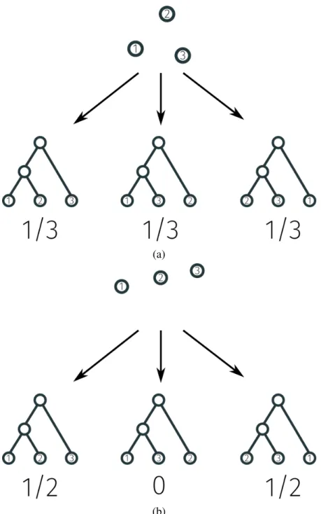
Figure 2.4: Examples of how Bayesian structure learning could uncover ambiguity in latent structure. In (a), all three possible clusterings are given equal probability and in (b), the two most likely clusterings split the probability.

(27)

τ

x1:N

Figure 2.5: The graphical model for Bayesian structure learning. Note the addition of a prior distribution over the structure.

strategy (variational inference, MCMC, etc.).

2.2.1

Bayesian linear dynamical system

A Bayesian linear dynamical system (BLDS) is an LDS with the addition of a prior over the transition matrix and noise covariance. Although there are many choices of prior, in this thesis, we use the matrix-Normal-inverse-Wishart (MNIW) prior, which is conjugate, details of which are located in section A.7.

The choice of this prior results in a generative model

F,ΣΣΣ∼MNIW(Ψ,F0,V,ν)

st+1|st,F,ΣΣΣ∼N(Fst,ΣΣΣ)

which is also visualized in Figure 2.6.

s1 s2 sT

F,ΣΣΣ

N _‘

Figure 2.6: The graphical model for a Bayesian linear dynamical system. Note the addition of a prior over the dynamics parameters.

(28)

the posterior distribution p(F,ΣΣΣ| {s(₁n), . . . ,s(_Tn)}N_n₌₁)is also MNIW and can be computed in closed form. This structure class is explored in more detail in Chapter 9.

Another structure class of interest is trees, specifically hierarchical clusterings. In the next chapter, we detail how hierarchical clustering can be formalized in the Bayesian structure learning framework.

(29)

Chapter 3

Bayesian Nonparametric Hierarchical

Clustering

Most hierarchical clustering algorithms produce a binary tree over the data, where each leaf corresponds to a data point. Internal nodes correspond to groupings of descendant leaves. This approach is simple, but can run into problems when the hierarchical structure in the data is ambiguous. Consider a simple dataset with three points that are equidistant from each other or a dataset with three points lying equally spaced apart in a line (see Figure 2.3). A single binary tree is not sufficient to describe the similarity relationships between the points, as a single tree will imply that some points are more similar to each other than the other when they are in fact not. An initial solution is to extend clustering algorithms to produce trees with arbitrary branching factors. This will help solve the ambiguity problem in the first dataset, but not the second. Furthermore, we can construct adversarial datasets that will always be ambiguous. ConsiderNpoints lying on the unit circle, equally spaced apart. Due to rotational symmetry, there will be several equivalent trees with max branching factor less thanN. Since anN-ary tree overN data points implies no underlying structure, we require an approach that can handle ambiguity without compromising the capacity to

(30)

discover structure.

Bayesian nonparametric hierarchical clustering (BNHC) addresses the general issue of ambiguity in hierarchical structure by explicitly modeling any uncertainty with probability. Rather than outputting a single tree as in traditional hierarchical clustering, a Bayesian method returns a probability distribution over hierarchies that explain the data. In the ambiguous dataset with three points described earlier, a Bayesian method would return a distribution over the three hierarchies, where each is assigned a probability of 1/3. BNHC also follows the standard Bayesian paradigm, where Bayes rule enables calculating a posterior distribution given a prior and a likelihood model.

3.1

Background

In this section, we briefly discuss some traditional hierarchical clustering algorithms and provide some background knowledge on latent variable modeling.

3.1.1

Traditional hierarchical clustering

Traditional hierarchical clustering algorithms can be broadly divided into two categories:agglomerative(bottom-up) anddivisive(top-down). In agglomerative clustering, the hierarchy is built by iteratively merging clusters that are most similar to each other, forming larger and larger clusters at each level of the tree. In divisive clustering, the hierarchy is built by recursively splitting the data from the top, forming a new pair of nodes with each split (Hastie et al., 2009).

The input to hierarchical clustering algorithms is a dataset,x1:N. The output is aτ,

a rooted tree withN labeled leaves, each corresponding to one of the data points. Typically, the tree is binary and internal nodes correspond to groupings of the leaves of the tree.

(31)

and alinkage criterion. A dissimilarity function,d(xi,xj)measures how different two data

pointsx_i andx_j are from each other; for example, we may choose Euclidean distance if our data are real valued vectors. A linkage criterionD(A,B)measures how different two clustersAandBare from each other in terms of the pairwise dissimilarities between the points in each cluster. A popular linkage criterion issingle linkage, which defines cluster dissimilarity as that of the closest points in each cluster, i.e.

D_SL(A,B) = min

i∈A,j∈Bd(xi,xj) (3.1)

Another common linkage function is average linkage, where cluster dissimilarity is the mean dissimilarity between all pairs of points in each cluster.

DAL(A,B) = 1

|A||B|_i∈A

∑

_,_j∈Bd(xi,xj) (3.2)

Finally, incomplete linkage, the cluster dissimilarity is that of the furthest points in each cluster, the opposite of single linkage.

D_CL(A,B) = max

i∈A,j∈Bd(xi,xj) (3.3)

Agglomerative clustering begins by instantiating a singleton cluster{n}for eachxn,

which will be the leaves of our output hierarchy. Every iteration of the algorithm, we find the two least dissimilar clustersAandBaccording to the linkage criterion and merge them, producing a new cluster. AfterN−1 iterations, we are left with a single cluster containing all the data, and the process creates a binary tree where each internal node correspond to one of the merge operations.

See examples of clusterings with each linkage criterion in Figure 3.1.

(32)

Figure 3.1: Hierarchies over human tumor data produced by agglomerative clustering with three different linkage criteria. Image from Hastie et al. (2009).

every data point, corresponding to the root of the output tree. We recursively partition the cluster, until we are left with singleton clusters at each leaf. Partitioning a cluster typically corresponds to solving an optimization problem, such as minimizing a cost function of a split. For example, we could partition a cluster usingk-means, withk=2, optimizing the k-means cost function. Alternatively in spectral clustering methods, we create a similarity graph,G, given a similarity functions(x,x0). Gis an undirected, weighted graph where there is a node for each data point, and the weight for each edge(i,j)iss(x_i,x_j)(Von Luxburg, 2007). Bipartitioning a cluster corresponds to finding a cut in its similarity graph, and intuitively a good cut would avoid edges between similar points. Finding a good partition thus corresponds to finding a minimum cut onGfor such cost functions as RatioCut (Hagen and Kahng, 1992) and Ncut (Shi and Malik, 2000).

(33)

3.2

The generative process

Bayesian nonparametric hierarchical clustering (BNHC) is a latent variable model where data is generated in in two stages. First, a tree is generated by atree prior. Condi-tioned on the sample from the tree prior, data is generated with atree likelihood model.

The simplest tree priors modelcladograms, or rooted binary trees with data at the leaves, but very often the trees are imbued with additional information. For example:

1. An ordering on the internal nodes of the tree. Typically, the root is given the lowest number and each node will have a higher number than its parent.

2. Times associated with each node. Nodes higher up in the tree will typically have earlier times, creating an evolutionary interpretation to the hierarchy. Cladograms with times associated at each node are also calledphylogenies.

If we are only interested in tree structure, not ordering or node times, we can simply discard all auxiliary information at the very end.

τ

x1:N

Figure 3.2: The graphical model used in Bayesian hierarchical clustering.τ is a tree, sampled from a tree prior distribution.

Formally, let τ be a class of tree structures (e.g. ordered cladograms), and let

p(τ ∈ T) be a tree prior for T . We sample parameters θ for tree likelihood model,

conditional on the tree structure. This involves assigning latent parameters to each internal node in theτ and specifying a stochastic process in which they are generated. Conditioned

(34)

x1:N is generated via probability distribution p(x1:N|τ,θ). This is visualized as a graphical

model in Figure 3.2 and concisely expressed as follows:

τ ∼p(τ) θ ∼p(θ|τ)

x1:N ∼p(x1:N|τ,θ)

Inference involves computing the posterior distribution over trees and parame-ters, p(τ,θ|x1:N), but we are sometimes interested in the posterior marginal distribution

p(τ|x1:N). Both of these distributions are typically impossible to compute analytically as

marginalizing overτ is intractable. In practice, most methods use Markov chain Monte

Carlo methods to samplep(τ,θ|x1:N)and p(τ|x1:N).

In this section, we will cover two broad classes of tree priors and touch on some extraneous models. We will then explain a few tree likelihood models, and finish by explaining how to perform inference in Bayesian hierarchical clustering.

3.2.1

Tree priors

Broadly speaking, tree priors can be broadly broken down intocoalescentmodels anddiffusionmodels. Both of them share a core characteristic of being sequential models. In coalescent models, the tree is built sequentially from the bottom up. We begin with each data point in its own cluster, and sequentially merge clusters until there is only one. This idea is very similar to agglomerative clustering. Diffusion models take an inductive approach, where we begin with a hierarchy over a single data point, and sequentially add data to the hierarchy until we have a tree withN leaves, a fundamentally different paradigm.

(35)

Shared in both types of models is the property ofexchangeability. A sequence of random variables, x₁, . . . ,x_N, is considered exchangeable if their joint distribution is invariant to permutations of the variables. Exchangeability often enables computationally efficient inference algorithms.

Coalescent models: coalescent modeling was developed in the early 1980s by John Kingman, and achieved success in the field of population genetics (Kingman, 1982). Coalescent models assume a continuous time process, wherein individuals of a population are traced backwards in time through their ancestry until they all share a single common ancestor. In terms of hierarchical clustering, the individuals in the population correspond to a datasetx1:N, and their ancestry backwards in time is a hierarchy.

The classic coalescent model is Kingman’s coalescent (Kingman, 1982). It assumes a countably infinite population but has a consistency property which allows it to be described in terms of its marginal distribution over finite populations.

Consider a datasetx1:N withN points, which we will call “individuals”. In

King-man’s coalescent, our current population exists at timet=0, and each individual in the population has a single parent in the previous generation, which has its own parent, con-tinuing backwards in time untilt=−∞. At some time in the past, the lineage of any two individuals will “coalesce” when they share an ancestor. The lineages of the members of the population can be concisely described by thegenealogyfunction,π(t), that maps

between timetand a partition of{1, . . . ,N}that groups individuals together if their lineages have coalesced at timet. π(0) ={{1},{2}, . . . ,{N}}represents the current time, when no

lineages have coalesced. π(−∞) ={{1,2, . . . ,N}}is the partition of all individuals into a single group, when they all share a common ancestor (Teh et al., 2008).

Kingman’s coalescent is a probability distribution over genealogy functionsπ(t)

for populations of size∞, and the marginal distribution for populations of sizeN is called theN-coalescent. TheN-coalescent is a continuous-time Markov process over the space

(36)

of partitions of size N, starting at time t =0 with π(0) ={{1},{2}, . . . ,{N}}, going backwards untilt=−∞, withπ(−∞) ={{1,2, . . . ,N}}.

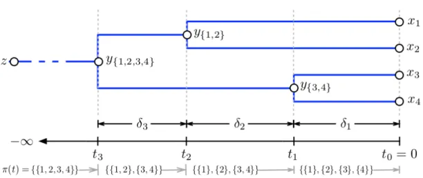
Figure 3.3: A sample from Kingman’s coalescent.zis the common ancestor for datax_1:4. Each yC represents the common ancestor for data subsetC. The axis represents time, and eachδi represents elapsed time.π(t)is the genealogy function. Image from Teh et al. (2008).

TheN-coalescent can be broken down into two independent components. The first is thejump process, which models the discrete transitions between partitions before and after coalesce events. The second is thetime process, which models the times in the past at which coalesce events happen. The jump process is very simple. Each lineage has an equal probability of merging with any other lineage. Thus, the jump process is a Markov chain where the transition matrix is uniform for each pair in a partition coalescing. The jump process hasN−1 transitions, starting with the partition with singleton groups for each data, and ending with the partition with all data in a single group. The time process produces a series of timest_N−₁<t_N−₂<· · ·<t₁when coalesce events happen, ending witht₀=0. The first step in the jump process corresponds to coalesce timet1, and so on. Kingman’s coalescent assumes that each pair of lineages merges at a constant rate of 1, i.e. a pair lineages will eventually merge att ∼Exp(1) where Exp is the exponential distribution.

(37)

Given a set ofmlineages, a pair of them will merge att∼Exp( m₂). Let the elapsed time before each jumpibeδi=ti−1−tiWe start with a population of sizeN, and it decreases

by 1 in each step of the jump process. Thus,δi∼Exp( N−i₂+1

). After sampling all the

δi’s, we can easily compute the coalesce times, completing the distribution over genealogy

functions. An example sample from Kingman’s coalescent can be seen in Figure 3.3.

Figure 3.4: For the balanced tree on the left, there are two possible orderings in which clusters were merged, whereas there is only one possible ordering for the unbalanced tree on the right. Image taken from Boyles and Welling (2012).

A genealogy sampled from Kingman’s coalescent is an ordered cladogram with times associated with every internal node. The ordering comes from the order in which internal nodes were created in the jump process. The induced distribution over just ordered trees is in fact uniform (Teh et al., 2008). However, we often don’t need order information in hierarchical clustering. Boyles and Welling (2012) computes the induced distribution over unordered rooted binary trees. For a given unordered tree withN leaves,τ, there are

(N−1)!

∏N_n=−11mn possible orderings where

m_n is the number of internal nodes in the subtree ofτ

indexed byn. Intuitively, there are several possible orderings to create a perfectly balanced binary tree, but only one for an extremely unbalanced binary tree (see Figure 3.4). Thus, Kingman’s coalescent induces a prior distribution over unordered trees that favors balanced trees over unbalanced trees, and marginalizing out the ordering of internal nodes results in this distribution, also called the time-marginalized coalescent (TMC; Boyles and Welling, 2012).

(38)

Kingman’s coalescent assumes constant merge rates for each pair of lineages in a genealogy. Although this is an intuitive assumption, there have been several papers generalizing Kingman’s coalescent to bothk-ary trees, and more complex coalesce rates. For example, in Pitman (1999), Pitman introduced theΛ-coalescent, extending Kingman’s coalescent to have “multiple collisions”, supportingk-ary trees. Rather than the coalesce rate being 1, it is insteadλ_ikwherekis the maximum number of lineages that can merge

in a single event andiis the total number of lineages at the time of the event, resulting in

δi∼Exp(λ_ik). λ_ikis calculated as

λ_ik=

Z 1

0

γk−2(1−γ)(i−k)Λ(dγ) (3.4)

whereΛis a finite measure on[0,1]. TheΛ-coalescent is identical to Kingman’s coalescent whenk=2 andΛis the Dirac delta. SettingΛto a beta measure results in the aptly named beta-coalescent (Hu et al., 2013). A description of such coalescent rate functions can be seen in Aldous (1999).

Diffusion models:diffusion models adopt a different paradigm for generation. In diffusion models, we begin with a trivial tree over just one data point. We then grow the tree by iteratively attaching new data to branches in the tree, eventually creating a tree with N leaves. Similar to coalescent models, there is an underlying continuous time process responsible for the tree structure.

The first diffusion model, the Dirichlet diffusion tree (DDT), was proposed in Neal (2003). The DDT is an exchangeable model that models a sequence of datax₁,x₂, . . . ,x_N. There is an underlying continuous time process that lasts from timet=0 tot=1 In essence, each data point is generated in sequence by a random walk beginning att =0, reaching a final value att =1. Each data point initially follows the previous random walks, but eventually diverges and continues independently.

(39)

Letxn(t)be the value of data pointxnat timet, defining a “path” associated with

each point from its startx_n(0)to its final (observed) value x_n(1). In addition, the path of each data pointx_n(t)is conditioned on all previous pathsx₁(t),x₂(t), . . . ,x_n−₁(t). This process, when completed for allNdata points, induces a binary tree over the data.

The path for the first data pointx₁is a Brownian motion beginning at the origin.

x₁(0) =0 (3.5)

x1(t+dt) =x1(t) +N(0,σ2Idt) (3.6)

The path for the second data pointx₂(t) is exactly x₁(t) until at some time τ it

diverges, creating a branching point for x₁(t) and x₂(t). τ is sampled according to an

acquisition function a(t)and after divergence,x₂(t)is an independent Brownian motion. Now consider the inductive case. We have already sampled n−1 paths, which form a binary tree with internal nodes corresponding to divergence events. xn(t)initially

follows the same path as the previous points, picking branches to follow proportional to the number of points that followed the branch previously. This scheme is called path reinforcementand encourages big subtrees to grow even bigger. Ifx₁(t)is traversing a path followed bymprevious paths, the probability thatx₁(t)will diverge along an infinitesimally small intervaldisa(t)dt/m. In practice we work with the cumulative divergence function A(t) =Rt

0a(u)du. Given an interval of time(s,t), that lies on a single branch of the DDT that was previously traversed bympaths, the probability that the next point does not diverge on the interval ise(A(s)−A(t))/m. The acquisition function is chosen such thata(1) =∞. This guarantees that all data points must diverge beforet=1. For a visualization of a DDT for 1-dimensional data, see Figure 3.5. Possible choices of acquisition function area(t) = ₁_−tc

ora(t) =b+ d

(40)

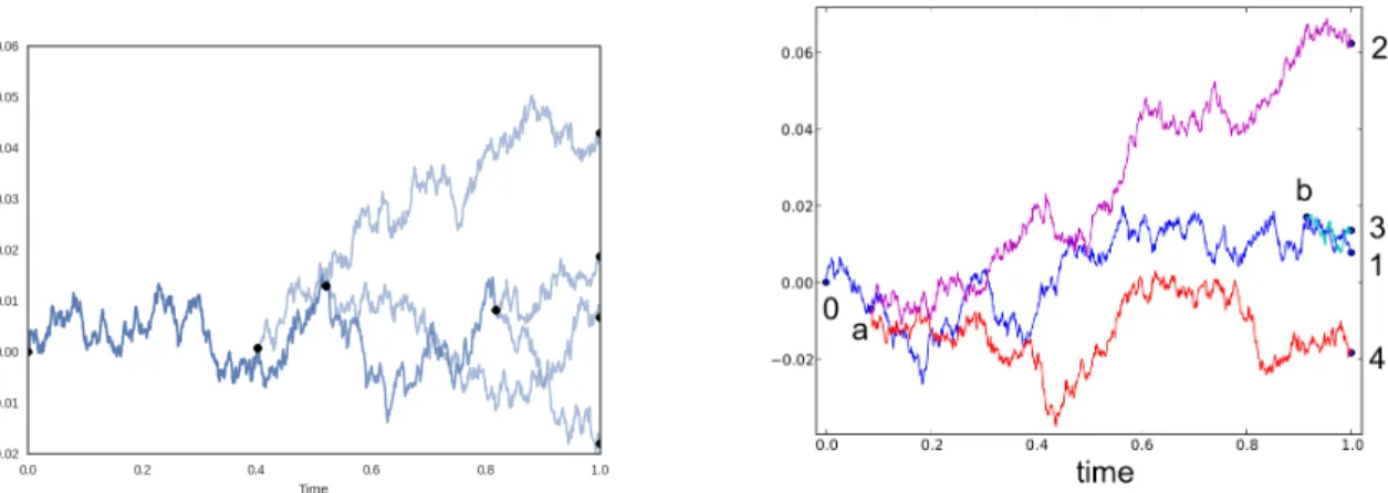
Figure 3.5: On the left is a sample Dirichlet diffusion tree. Black dots correspond to nodes in the tree. The image is taken from Vikram and Dasgupta (2016). On the right is a sample from a Pitman-Yor diffusion tree with 4 points. The image is taken from Knowles and Ghahramani (2015).

The DDT, as proposed in Neal (2003), jointly models the tree prior and tree likeli-hood model, as in it jointly samples tree structure and real-valued data associated with the tree. However, we can consider the same path reinforcement model, without the Brownian motion to obtain a prior over ordered cladograms with times for each node. We can obtain a sample from the DDT and just ignore the internal values at each node where divergence occurred.

The DDT thus induces a prior over ordered cladograms with times. Unlike King-man’s coalescent, however, the DDT does not, in general, induce a uniform prior over ordered cladograms. This is due to the path-reinforcement element of the prior and the choice of acquisition function. It is worth noting that the Dirichlet diffusion tree has achieved great success in the area of density estimation (Adams et al., 2008).

An extension to the Dirichlet diffusion tree is the Pitman-Yor diffusion tree (PYDT), which removes the DDT’s restriction to just binary trees (Knowles and Ghahramani, 2015). In a Pitman-Yor diffusion tree, the probability of a data point diverging in an infinitesimally

(41)

small intervaldt is

a(t)Γ(m−β)

Γ(m+1+α) (3.7)

whereα andβ are parameters. Setting α =β =0, results in same probability as in the

DDT. In the PYDT, a data point can not only diverge at any point in time, but can also diverge at a branching point in the tree, where in the DDT a data point would always pick a branch. When a data point reaches a branching point, it picks branchkwith probability

b_k−β

m+α (3.8)

whereb_kis the number of paths that previously traversedkandmis total the number of paths that reached the branching point. The probability that the data point diverges, creating a new branch, is

α+βK

m+α (3.9)

whereK is current number of branches. This scheme allows for an arbitrary amount of branching at each internal node of the tree, but can be tuned by settings ofα andβ. Note

again that whenα=β =0, the generation scheme matches the DDT.

3.2.2

Generalizations of coalescent and diffusion models

The simplest distribution over (unordered) cladograms is the uniform. Kingman’s coalescent is one step away, as it induces the uniform distribution over ordered cladograms, a distribution also called the Yule model (Harding, 1971). Marginalizing over possible orderings results in the TMC (Boyles and Welling, 2012), a distribution over unordered

(42)

cladograms biased towards balanced trees.

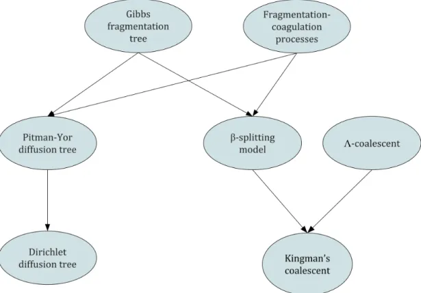
Generalizations of Kingman’s coalescent include theΛ-coalescent (Pitman, 1999), which extends coalescents to multifurcating trees, and the Aldousβ-splitting model (Aldous

and Pemantle, 1996). A more recent model, the Gibbs fragmentation tree, is a generaliza-tion of theβ-splitting model to multifurcating trees, and is considered the most general

Markovian distribution over trees (McCullagh et al., 2008).

The diffusion models on the other hand, include far more parameters. The choice of acquisition function, along with the choice ofα andβ in the PYDT, result in a wider

variety of distributions. The PYDT’s induced distribution over tree structure is, in fact, a specific case of the Gibbs fragmentation tree.

An alternate generalization is the fragmentation-coagulation process (FCP), which is a distribution over partition-valued Markov chains (Teh et al., 2011). Instead of partitions being split up or merged monotonically as in diffusion and coalescent models, the FCP models both split and merge transitions in the Markov chain, encompassing both coalescent and diffusion models.

(43)

Figure 3.6: A graph visualization of the relationships between various tree priors. Directed arrows represent specific cases of a distribution or model.

3.2.3

Other priors

A popular line of work follows extensions of the Chinese restaurant process (CRP) and other related Bayesian nonparametric objects. The CRP is a distribution over partitions of{1, . . . ,N}(Aldous, 1985). Its name derives from the nature of the stochastic process by which partitions are sampled. Imagine an empty restaurant with a countably infinite number of tables labeled 1,2, . . .with a line of customers waited to be seated. The first customer will always pick table 1. Letα be a hyperparameter. Then+1-th customer will

pick the thei-th table with probability

c_i

(44)

Figure 3.7: A visualization of a sampled from a nested Chinese restaurant process (NCRP). Only three levels for 5 customers are shown. Image from Blei et al. (2010).

whereci is the number of customers already sitting at tableior sit at a new, unoccupied

table with probability

α

n+α (3.11)

AfterN customers have been seated, we have a partition over{1, . . . ,N}, where customers are grouped by the table they are seated at.

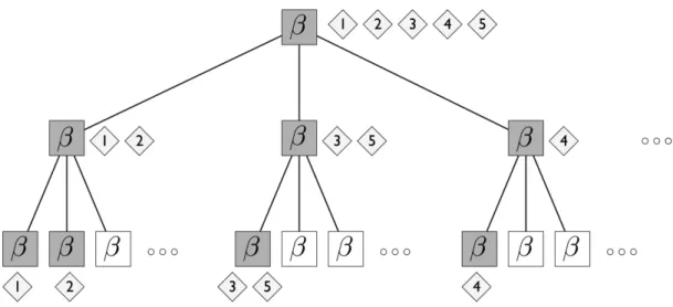
The CRP is an exchangeable model and has a reinforcement property, where tables with more people attract even more people. It is also the basis of the nested Chinese Restaurant Process (nCRP) model used for hierarchical clustering (Blei et al., 2010). The nCRP extends the analogy to an infinite chain of restaurants. After a customer goes and sits at the first Chinese restaurant, they are directed to yet another Chinese restaurant where the process repeats ad infinitum. This defines a structure where N customers, or data, are distributed across infinitely deep leaves of a tree. Although the tree is infinite, it can be represented in terms of its finite induced distribution over how the partition of

(45)

customers is split at each level of the tree. This results in a distribution over rooted trees with arbitrary branching factor and ordering over internal nodes. See Figure 3.7 for a visualization of the NCRP. The NCRP is closely related to the nested Dirichlet process (NDP), the underlying de Finetti measure for the NCRP. An extension of the NCRP and NDP is the nested hierarchical Dirichlet process (NHDP) (Paisley et al., 2014). Whereas each datum in the NDP and NCRP are each represented as an infinitely deep path down the tree, each datum in the NHDP is represented as amixtureof infinitely deep paths down the tree. The NCRP, NDP, and NHDP have been used to success in topic modeling, finding hierarchies over a corpus of documents.

The tree-structured stick-breaking process (TSSB) is an alternate model where data are allowed to live at any node in the tree, as opposed to just leaves (Adams et al., 2010). At the core of the TSSB is the stick-breaking process, a Bayesian nonparametric object closely related to the CRP. The stick breaking process iteratively carves up the unit interval into smaller and smaller pieces, resulting in an infinite amount of “sticks”, whose lengths sum up to one. Letβi∼Beta(1,α)fori∈1,2, . . .. These will be fractions of the remainder

of the stick that we will carve up. Now, let the “sticks” bet₁=β1andti=βi∏ij=1(1−βj).

We now have a sequence of random variables,t₁,t₂, . . .such that∑∞i=1ti=1, which we can

treat as a distribution over an infinite amount of events. The TSSB is an extension of the stick-breaking process to generate a distribution over infinitely deep and wide hierarchies. Associated with each internal node in the tree is a stick breaking process, which acts as a distribution over an infinite amount of branches out of the node. Data are generated by starting at the root and sampling a branch. At any point, data have a probability of stopping at a given node, which distributed as a stick breaking process over each possible path heading down the tree. Although the tree is infinite, it induces a distribution over trees whereN data live across every node in the tree, a fundamentally different tree structure from the previous ones.

(46)

3.2.4

Tree likelihood models

Given a sample from a tree structure prior, we now need a scheme to sample hierarchically structured data. Let the sample from the tree structure prior beτ. Assume,

for now,τ is an rooted tree, with times associated with each internal node (ordering does

not matter). The standard tree likelihood model is a diffusion model, where there is a parameterθnfor each internal noden, which are generated from the root downwards. Let

θ0be the parameter associated with the root node, which will be sampled according to a prior distribution p0(θ). We then define a transition kernel,T(θ0|θ). The parameter for

each node is generated conditionally given its parent parameter in the tree, i.e. for node vand its parent u,θv∼T(· |θu). Data at leaves are also generated in this fashion. We

now enumerate some transition kernels which accommodate different data types and tree structures.

1. Generalized Gaussian diffusion.If our data is continuous andD-dimensional, we can associate a latent vectorθn∈RDwith each internal nodenin the tree. Letube an

internal node andvone of its children and letδuvbe the elapsed time betweenuand

v. We sampleθv∼N(θu,Σδuv), whereΣis a positive definite covariance matrix. The root node value is assigned a priorN(µ0,Σ0). In the case where there are no times associated with each node, we can assume elapsed time between nodes is always 1, and the hyperparameters in the model would beΣ,µ0, andΣ0. This approach is used in Neal (2003), Teh et al. (2008), Knowles and Ghahramani (2015), Adams et al. (2010), Boyles and Welling (2012) and Hu et al. (2013).

2. Multinomial diffusion. If our data consists of several categorical variables, we can model it with a transition matrix,τ. For categorical featurec, letTcbe the row inτfor

featurec. Letδuvbe the elapsed time between parentuand childv. As suggested by

Teh et al. (2008),T_c=e−λcδuv_I_{+ (}₁₋_e−λcδuv₎_qT

(47)

the evolution rate for featurec,qcis a hyperparameter for the equilibrium distribution

ofc, and 111 is a vector of ones.

3. Dirichlet-Multinomial diffusion. This tree likelihood model is for trees without times associated with each internal node. When data consists of counts of discrete events, such as the bag of words in topic modeling, leaves can be described as sampling a multinomial distribution. The transition kernel for just internal nodes as suggested by Adams et al. (2010) isT(θ0|θ) =Dirichlet(κ θ) and the prior is

P₁(θ) =Dirichlet(κ111), whereκ is a concentration hyperparameter and 111 is a vector

of ones. Leaves are sampled via a multinomial distribution with its parent’s vector as its parameter.

3.2.5

Inference

We are interested in the posterior distribution over hierarchies given data. Typically, this distribution is intractable to compute analytically, so approximate methods are required. A popular approach used in Neal (2003), Knowles and Ghahramani (2015), and Boyles and Welling (2012) is the Metropolis-Hastings algorithm, a Markov chain Monte Carlo method where samples are used as an approximation to the posterior distribution.

In Metropolis-Hastings, we are given a target distribution, p(x), and define a proposal distribution,q(x0|x). A Markov chain is initialized with statex₀. In each iteration of the algorithm we use current statex_t to sample a candidatex0fromq(x0|x_t). and then calculate the acceptance ratio,

α= p(x

0₎_q₍_x t|x0)

p(xt)q(x0|xt)

(3.12)

(48)

Figure 3.8: Visualization of a subtree-prune and regraft move for a tree with four leaves. Image from Vikram and Dasgupta (2016).

otherwise, setting xt+1=xt. Provided some conditions on q(x0|x), the Markov chain’s

stationary distribution will be p(x).

In BNHC, the probability distribution of interest is the posterior distribution p(τ,θ|x1:N). The state of a Markov chain in Metropolis-Hastings is therefore a tuple (τ,θ). A proposal distributionq(τ0,θ0|τ,θ,x1:N)would need to jointly sampleτ andθ. A

simple strategy is to have two proposal distributions: a tree proposalq(τ0|τ)and parameter

proposalq(θ0|τ0,θ). We would sampleτ0first, and then we would sampleθ0additionally

conditioned onτ0. Alternatively, if we’re only interested the posterior distribution over

trees, we can often marginalize outθ, either analytically or via belief propagation, resulting

in the posterior marginal distribution p(τ|x1:N).

Designing a tree proposal distribution involves modifying some treeτ randomly

to form a new treeτ0. One of the most popular proposals is thesubtree-prune and regraft

(SPR) move, proposed by Swofford and Olsen (1990). An SPR move consists of aprune followed by aregraft. Letτ be a tree. Letsbe a non-root node inτ selected uniformly at

random andSbe its corresponding subtree. We firstprune Sfromτ by removes’s parent p

from the tree, replacingpwiths’s sibling. To regraftptoτ, we first select a branch inτ,

(u,v), whereuis the parent ofv. Sis re-attached toτ by creating a new node pwith parent

(49)

The branch selected in the regraft move is often sampled from a distribution related to the tree prior. For example, if we used a DDT, we have a posterior distribution over branches where a new data point would diverge. If such a distribution does not exist, the branch can simply be selected uniformly at random.

Two alternatives to the SPR move moves are the leaf move, which restricts the SPR move to just leaf nodes, and nearest-neighbor interchange moves, which interchange two pairs of subtrees. It is worth noting that the worst case mixing rate of a Markov chain using leaf moves to sample the uniform distribution overN-leaf cladograms isO(N3)(Aldous, 2000).

Sampling the parameters of the tree likelihood model is much simpler than sampling the tree prior. The parametersθ often have conditional dependence structure that allows

simple ancestral sampling or Gibbs sampling. For example, in the DDT and Kingman’s coalescent, each internal node in the tree stores a latent vector, representing the intermediate value of data higher up in the tree. If the likelihood model is generalized Gaussian diffusion, all conditional distributions are Gaussian. We can thus Gibbs sample each of the latent vectors.

Metropolis-Hastings is perhaps the simplest method to sample a general BNHC model. However, alternative methods have been proposed, such as using slice sampling in Adams et al. (2010) and Boyles and Welling (2012), sequential Monte Carlo in Teh et al. (2008) and Hu et al. (2013), Gibbs sampling in Blei et al. (2010), and variational inference in Paisley et al. (2014). Furthermore, there are greedy algorithms to approximate a MAP estimate to the posterior distribution of trees given data (Teh et al., 2008; Hu et al., 2013).

(50)

Chapter 4

Interactive Bayesian Hierarchical

Clustering

Clustering is a basic tool of exploratory data analysis. There are a variety of efficient algorithms—includingk-means, EM for Gaussian mixtures, and hierarchical agglomerative schemes—that are widely used for discovering “natural” groups in data. Unfortunately, they don’t always find a grouping that suits the user’s needs.

This is inevitable. In any moderately complex data set, there are many different plausible grouping criteria. Should a collection of rocks be grouped according to value, or shininess, or geological properties? Should animal pictures be grouped according to the Linnaean taxonomy, or cuteness? Different users have different priorities, and an unsupervised algorithm has no way to magically guess these.

As a result, a rich body of work on constrainedclustering has emerged. In this setting, a user supplies guidance, typically in the form of “must-link” or “cannot-link” con-straints, pairs of points that must be placed together or apart. Introduced by Wagstaff et al. (2001), these constraints have since been incorporated into many differentflatclustering procedures (Wagstaff and Cardie, 2000; Bansal et al., 2004; Basu et al., 2004; Kulis et al.,

(51)

2009; Biswas and Jacobs, 2014).

In this chapter, we introduce constraints tohierarchical clustering, the recursive partitioning of a data set into successively smaller clusters to form a tree. A hierarchy has several advantages over a flat clustering. First, there is no need to specify the number of clusters in advance. Second, the tree captures cluster structure at multiple levels of granularity, simultaneously. As such, trees are particularly well-suited for exploratory data analysis and the discovery of natural groups.

There are several well-established methods for hierarchical clustering, the most prominent among which are the bottom-up agglomerative methods such as average linkage (see, for instance, Chapter 14 of Hastie et al. (2009)). But they suffer from the same problem of under-specification that is the scourge of unsupervised learning in general. And, despite the rich literature on incorporating additional guidance into flat clustering, there has been relatively little work on the hierarchical case.

What form might the user’s guidance take? The usual must-link and cannot-link constraints make little sense when data has hierarchical structure. Among living creatures, for instance, shouldelephantandtigerbe linked? At some level, yes, but at a finer level, no. A more straightforward assertion is thatelephantandtigershould be linked in a clus-ter that does not includesnake. We can write this as atriplet({elephant,tiger},snake). We could also assert({tiger,leopard},elephant). Formally,({a,b},c)stipulates that the hierarchy contains a subtree (that is, a cluster) containingaandbbut notc.

A wealth of research addresses learning taxonomies from tripletsalone, mostly in the field of phylogenetics: see Felsenstein (2004) for an overview, and Aho et al. (1981) for a central algorithmic result. Let’s say there areNdata items to be clustered, and that the user seeks a particular hierarchyτ∗on these items. Thisτ∗embodies at most N₃triplet

constraints, possibly less if it is not binary. It was pointed out in Tamuz et al. (2011) that roughlyNlogN carefully-chosen triplets are enough to fully specifyτ∗if it is balanced.

(52)

This is also a lower bound: there are NΩ(N) _{different labeled rooted trees, so each tree} requiresΩ(NlogN)bits, on average, to write down—and each triple providesO(1)bits of information, since there are just three possible outcomes for each set of pointsa,b,c. AlthoughNlogN is a big improvement overN3, it is impractical for a user to provide this much guidance when the number of points is large. In such cases, a hierarchical clustering cannot be obtained on the basis of constraints alone; the geometry of the data must play a role.

We consider an interactive process during which a user incrementally adds con-straints.

• Starting with a pool of datax1:N ⊆RD, the machine builds a candidate hierarchyτ.

• The set of constraintsCis initially empty.

• Repeat:

– The machine presents the user with a small portion of τ: specifically, its

restriction toO(1)leavesS⊂X. We denote thisτ|S.

– The user either accepts τ|S, or provides a triplet constraint ({a,b},c)that is

violated by it.

– If a triplet is provided, the machine adds it toCand modifies the treeT accord-ingly.

In realizing this scheme, a suitable clustering algorithm and querying strategy must be designed. Similar issues have been confronted in flat clustering—with must-link and cannot-link constraints—but the solutions are unsuitable for hierarchies, and thus a fresh treatment is warranted.

The clustering algorithm: What is a method of hierarchical clustering that takes into account the geometry of the data points as well as user-imposed constraints?

(53)

We adopt aninteractive Bayesianapproach. The learning procedure is uncertain about the intended tree and this uncertainty is captured in the form of a distribution over all possible trees. Initially, this distribution is informed solely by the geometry of the data but once interaction begins, it is also shaped by the growing set of constraints.

The nonparametric Bayes literature contains a variety of different distributional models for hierarchical clustering. We describe a general methodology for extending these to incorporate user-specified constraints. For concreteness, we focus on the Dirichlet diffusion tree (Neal, 2003), which has enjoyed empirical success. We show that triplet constraints are quite easily accommodated: when using a Metropolis-Hastings sampler, they can efficiently be enforced, and the state space remains strongly connected, assuring convergence to the unique stationary distribution.

The querying strategy: What is a good way to select the subsets S? A simple option is to pick them at random fromx_1:_N. We show that this strategy leads to convergence to the target treeτ∗. Along the way, we define a suitable distance function for measuring

how closeτ is toτ∗.

We might hope, however, that a more careful choice of S would lead to faster convergence, in much the same way that intelligent querying is often superior to random querying in active learning. In order to do this, we show how the Bayesian framework allows us to quantify which portions of the tree are the most uncertain, and thereby to pick Sthat focuses on these regions.

Querying based on uncertainty sounds promising, but is dangerous because it is heavily influenced by the choice of prior, which is ultimately quite arbitrary. Indeed, if only such queries were used, the interactive learning process could easily converge to the wrong tree. We show how to avoid this situation by interleaving the two types of queries.

Finally, we present a series of experiments that illustrate how a little interaction leads to significantly better hierarchical clusterings.

(54)

Other related work

A related problem that has been studied in more detail (Zöller and Buhmann, 2000; Eriksson et al., 2011; Krishnamurthy et al., 2012) is that of building a hierarchical clustering where the only information available is pairwise similarities between points, but these are initially hidden and must be individually queried.

In another variant of interactive flat clustering (Balcan and Blum, 2008; Awasthi and Zadeh, 2010; Awasthi et al., 2013), the user is allowed to specify that individual clusters be merged or split. A succession of such operations can always lead to a target clustering, and a question of interest is how quickly this convergence can be achieved.

Finally, it is worth mentioning the use of triplet constraints in learning other struc-tures, such as Euclidean embeddings (O’Connell et al., 1999).

4.1