Efficient Generation of Power In Medium Voltage Direct Current Systems: Variable Speed Operation and Rectifier Considerations

(1)

University of South Carolina

Scholar Commons

Theses and Dissertations

1-1-2013

Models and Software Development For

Interval-Censored Data

Chun Pan

University of South Carolina

Follow this and additional works at:https://scholarcommons.sc.edu/etd Part of theBiostatistics Commons

This Open Access Dissertation is brought to you by Scholar Commons. It has been accepted for inclusion in Theses and Dissertations by an authorized administrator of Scholar Commons. For more information, please [email protected].

Recommended Citation

(2)

Models and Software Development for Interval-Censored Data

by

Chun Pan

Bachelor of Science Nanjing University 2001

Master of Science Nanjing University 2004

Master of Science

University of South Carolina 2009

Submitted in Partial Fulfillment of the Requirements

for the Degree of Doctor of Philosophy in

Biostatistics

Arnold School of Public Health

University of South Carolina

2013

Accepted by:

Bo Cai, Major Professor

Lianming Wang, Committee Member

Jiajia Zhang, Committee Member

Andrew Ortaglia, Committee Member

(3)

c

(4)

Acknowledgments

This dissertation is a summary of the research work I have done under the supervision

of my advisor Dr. Bo Cai. I am deeply grateful to him for his insightful, intelligent,

and patient guidance and his creative suggestions when I encountered difficuties in

the past three years. I sincerely appreciate all of his great support along the way as

I would not be able to make it without him.

I am very grateful to Dr. Lianming Wang for instructing me with his expertise

on interval-censored data. I have learned a lot about the concept and modeling

methodology for this type of data by meeting with him and studying his R programs

and publications.

I would like to express my sincere gratitude to Dr. Jiajia Zhang for her

enlight-ening comments on my work. Especially worth to mention, I have been stuck at my

second project for months and one day Dr. Zhang’s comment solved the riddle for

me immediately.

Dr. Andrew Ortaglia has gone through the writing of my dissertation in detail.

Also he has been so cordial and supportive both during the completion of the

dis-sertation and during my course study, which has really encouraged me a lot when I

came to barriers.

I also would like to thank Dr. Suzanne McDermott and Dr. Joshua Mann for

their financial support and advice during my PhD study. Finally, I thank my parents

(5)

Abstract

Interval-censored time-to-event data occur naturally in studies of diseases where the

symptoms are not directly observable, and periodic lab or clinical examinations are

re-quired for detection. Due to the lack of well-established procedures, interval-censored

data have been conventionally treated as right-censored data, however, this

intro-duces bias at the first place. This dissertation focuses on methodological research

and software development for interval-censored data. Specifically, it consists of three

projects. The first project is to create an R package for regression analysis and

sur-vival curve estimation of interval-censored data based on several published papers

by our research team. In the second project, a Bayesian semiparametric

propor-tional hazards model with spatial random effect is developed for spatially correlated

interval-censored data. In the third project, we propose a multivariate frailty model

for clustered interval-censored failure times, which is analogous to a mixed model in

(6)

List of Tables

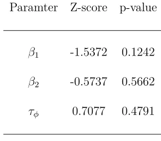
Table 4.1 Geweke’s convergence diagnostic for MCMC chains of the model

parameters in the 1st simulated dataset . . . 47

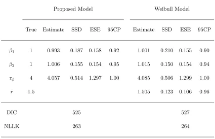
Table 4.2 Estimation results for simulation 1 . . . 47

Table 4.3 Estimation results for simulation 2 . . . 50

parameters in the smoke-relapse data . . . 55

Table 4.5 Estimation results for the smoking cessation study . . . 56

parameters in the 1st simulated dataset . . . 69

Table 5.2 Posterior homogeneity probabilities and Bayes factors of frailties

in the simulation study . . . 70

Table 5.3 Posterior probabilities of the 8 possible models in the simulation

study . . . 70

Table 5.4 Estimated fixed effects and coverage probabilities in the

simula-tion study . . . 70

Table 5.5 Geweke’s convergence diagnostic for MCMC chains of model

pa-rameters in the lymphatic filariasis study . . . 74

Table 5.6 Posterior homogeneity probabilities and Bayes factors of frailties

in the lymphatic filariasis study . . . 75

Table 5.7 Posterior probabilities of the 8 possible models in the lymphatic

filariasis study . . . 75

(9)

List of Figures

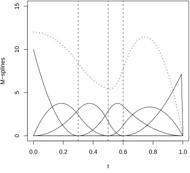
Figure 2.1 A set of M-splines with order = 3, t = {0,0.3,0.5,0.6,1}, and

f = 1.2M1+ 2.0M2+ 1.2M3+ 1.2M4+ 3.0M5+ 0.0M6 . . . 12

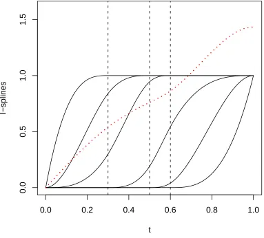
Figure 2.2 A set of I-splines with order = 3, t = {0,0.3,0.5,0.6,1}, and f = (1.2I1+ 2.0I2+ 1.2I3+ 1.2I4+ 3.0I5 + 0.0I6)/6 . . . 13

Figure 3.1 Traceplot of MCMC chain for β of case 2 PH model in breast cancer study . . . 25

Figure 3.2 Traceplot of MCMC chain forβof case 2 probit model in breast cancer study . . . 26

Figure 3.3 Estimated survival curves for two groups of patients in breast cancer study . . . 28

Figure 3.4 Traceplot of MCMC chain for β in case 1 PH model for lung cancer data . . . 30

Figure 3.5 Traceplot of the MCMC chain ofβ in case 2 PH model for lung cancer data . . . 32

Figure 3.6 Estimated survival curves for two groups of patients in lung cancer study . . . 33

Figure 4.1 A recent mapping of air pollution particle levels in China . . . 35

Figure 4.2 Traceplot of fixed effect β1 in the 1st simulated dataset. . . 45

Figure 4.3 Traceplot of fixed effect β2 in the 1st simulated dataset. . . 46

(10)

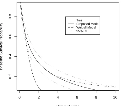
Figure 4.5 Plot of estimated baseline survival curve based on 100 simulated

data sets using proposed model (with 95% pointwise credible

in-tervals) and Weibull model, compared to true baseline survival

curve (simulation 1). . . 48

Figure 4.6 Maps of posterior means for the spatial random effects φi over 46

counties of SC based on proposed model and Weibull model

(simu-lation 1). . . 49

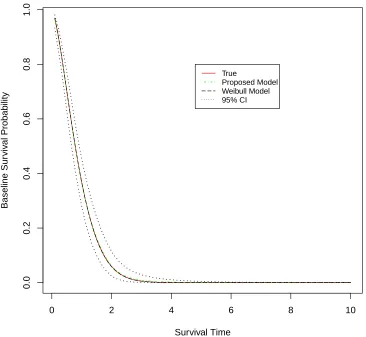
Figure 4.7 Plot of estimated baseline survival curve based on 100 simulated

data sets using proposed model (with 95% pointwise credible

in-tervals) and Weibull model, compared to true baseline survival

curve (simulation 2). . . 51

Figure 4.8 Traceplot of fixed effect β1 in the smoking-relapse data. . . 53

Figure 4.9 Traceplot of fixed effect β2 in the smoking-relapse data. . . 53

Figure 4.10 Traceplot of spatial precision τφ in the smoking-relapse data. . . . 54

Figure 4.11 Traceplot of spatial precision τφ in the smoking-relapse data. . . . 54

Figure 4.12 Estimated survival curves for the smoking cessation study, using

Turnbull method, proposed model, and Weibull model; event of

interest is time to relapse to smoking. Four curves are plotted

for each method based on the four subgroups formed by gender

and treatment. . . 57

Figure 4.13 Maps of posterior means for the spatial random effects φi over 51

zip codes areas in southeast Minnesota based on proposed model

and Weibull model. The other 32 zip code areas without data are

plotted in white color. . . 58

Figure 5.1 Traceplot of fixed effect β1 in simulation study. . . 67

(11)

Figure 5.3 Traceplot of the probability of homogeneity forξi1 in simulation

study. . . 68

study. . . 69

Figure 5.6 Traceplot of fixed effect β1 in lymphatic filariasis study. . . 72

Figure 5.7 Traceplot of fixed effect β2 in lymphatic filariasis study. . . 72

Figure 5.8 Traceplot of the probability of homogeneity forξi1 in lymphatic

filariasis study. . . 73

(12)

Chapter 1 Introduction

1.1 Interval-Censoring

Interval-censored data occur naturally in studies of diseases where the symptoms

of interest are not directly observable, and laboratrory or clinical examinations are

required for detection. The exact time to event of interest T is not directly observed,

but is known to fall within a time interval (L, R], such that 0≤L < T ≤R≤ ∞.

Consider in a tumorigenicity study, a lab animal has to be dissected to check

whether a tumor has developed. Let C denote the time of dissection, and T denote

the true tumor onset time, then the data observed is (C,1(T ≤C)). Then

(L, R] =

      

(0, C], T ≤C

(C,∞), T > C

(1.1)

This is called case 1 interval-censored or current status data.

Suppose there are two examination timesU andV for each subject, then the data

observed is (U, V, δ1 =I(T ≤U), δ2 =I(U < T ≤V)). Then

(L, R] =

              

(0, U], T ≤U

(U, V], U < T ≤V

(V,∞), T > C

(1.2)

This is the case 2 interval-censored data. Case k interval-censoring refers to when

there are k examination times per subject.

Consider another situation. In an oncology clinical trial for non-small cell lung

(13)

scanned by CT every couple of weeks for evaluation of tumor sizes and new lesions.

Then the scan results are read by a diagnostic radiologist to determine if progression

has occurred or not. Then PFS is interval-censored as the exact time to progression

is not observed but is known to fall within a time interval (L, R]. Suppose Oi =

{Oi1, . . . , Oi,ni}are the examination times for the ith patient, i= 1, . . . , n. Then

(L, R] =

              

(0, Oi,1], T ≤Oi,1

(Oi,L, Oi,R], Oi,L < T ≤Oi,R

(Oi,ni,∞), T > Oi,ni

(1.3)

This is called general interval-censoring, which includes case 1, case 2 and case k

interval-censoring as special cases. In the dissertation, we will focus on general

interval-censoring.

1.2 Likelihood function

Throughout the dissertation, we assume the following two basic assumptions (Huang

and Wellner, 1997). (A1) The failure time is independent of the examinations times

given the covariates. (A2) The distribution of the examination times does not involve

the parameters of interest.

Under these assumptions we can derive the likelihood function. For case 1, or

equivalently current status data, the joint density of a single observation (C, δ =

I(T ≤C),x) is:

f(δ, c,x) =f(δ|c,x)f(c,x) =f(δ|x)f(c,x)

=F(c|x)δ(1−F(c|x)1−δf(c,x)),

where F is the cdf of T. So for an independent sample of size n from the same

distribution, the likelihood function is proportional to:

L=

n

Y

i=1

n

(14)

For case 2 and general interval-censoring, let δ1,δ2, δ3 denote left-, interval-, and

right-censoring, the joint density of a single observation (δ1, δ2, δ3, L, R,x) is:

f(δ1, δ2, δ3, L, R,x) =f(δ1, δ2, δ3|L, R, x)f(L, R,x) = f(δ1, δ2, δ3|x)f(L, R,x)

=F(R|x)δ1₍_F₍_R_|_x₎₋_F₍_L_|_x₎₎δ2₍₁₋_F₍_L_|_x₎₎δ3_f₍_{L, R,}_x₎_.

The likelihood function for an independent sample of sizenfrom the same distribution

is proportional to:

L=

n

Y

i=1

n

F(Ri|xi)δ1i(F(Ri|xi)−F(Li|xi))δ2i(1−F(Li|xi))δ3i

o

.

1.3 Motivations

For interval-censored data, the conventional approach in pharmaceutical industry

treats the right-point of the time interval as the observed time, and then apply the

standard right-censored methods. However, this approach can lead to biased

estima-tion and invalid inferences (Rücker and Messerer, 1988; Odell et al., 1992; Lindsey

and Ryan, 1998; Sun and Chen, 2012). Better estimations can be obtained if the

information of interval censorship is taken into account in modeling.

Quite a few new methods for analysis of interval-censored time-to-event data have

been proposed in the last two decades. However, most of these methods either rely

on parametric assumptions that are hard to verify in practice or are computationally

challenging. As a result, none of them has been accepted by the pharmaceutical

industry as a standard procedure. We propose to model the survival function

semi-parametically through I-splines (Ramsay, 1988) and estimate survival function and

regression coefficients through Markov chain Monte Carlo (MCMC) algorithm. Our

models are relatively straightforward to implement in practice and give more accurate

estimates. Specifically, the dissertation research consists of three projects; each has

(15)

Currently, a few packages and SAS macros, mainly the ‘interval’ and ‘glrt’

pack-ages in R and the %EMICM and the %ICSTEST macros in SAS, have been developed

to provide estimation and comparison for survival functions for interval-censored data.

However, there are currently few options available for fitting regression models, except

the ‘survBayes’ package and the ‘intcox’ package. As the first project of this

disser-tation, we have built an R package, ICBayes, which fits proportional hazards (PH),

proportional odds (PO), and probit regression models from a Bayesian perspective.

It is possible that failure times of interest are both interval-censored and spatially

correlated. For instance, in a lung cancer clinical trial, patients are recruited from

a number of regions where air quality in a region is similar to that in its neighbors

but might differ substantially from that in the other regions. If air quality exerts

an effect on treatment outcome, then survival times of patients may be spatially

correlated. Only one spatial frailty model has been developed for such type of data

under parametric Weibull PH cure rate model (Banerjee and Carlin, 2004). We

propose a semiparametric spatial frailty PH model, which provides greater flexibility

for modeling failure time.

Clustered interval-censored survival data can easily occur in multicenter clinical

trials for cancer, HIV, or other infectious diseases. Tumor progression, HIV

progres-sion to AIDS, and presence/absence of an infection normally all need periodic lab

examinations for detection. Characteristics that vary by center may affect survival

times, which implies either an overall frailty to account for baseline hazard

hetero-geneity across centers or a frailty corresponding to a certain predictor to account for

center-wise variation of this predictor’s effect. We propose to model the variance of a

potential frailty with a mixture of point mass and gamma distribution, because rather

than arbitrarily assuming the heterogeneity structure, we want to actually estimate

(16)

Chapter 2 Background Knowledge

2.1 The Poisson Distribution and the Poisson Process

2.1.1 Additive Property of Poisson DistributionSuppose X1, . . . , Xn are

inde-pendent with Xi ∼Poisson(λi), i= 1, . . . , n, then

Yi =

n

X

i=1

Xi ∼Poisson(

n

X

i=1

λi).

This can be proved through the moment generating function method. This property

will be used in introducing Poisson latent variables in our data augmentation.

2.1.2 Poisson Process A Poisson process is a counting process in which events

occur continuously and independently of one another. Let N(t) be the number of

events in time interval (0, t]. The process{N(t), t≥0}is said to be a Poisson process

with rate (or intensity) λ, λ >0, if

• N(0) = 0.

• (independent increment) the number of events in non-overlapping intervals are

independent.

• (stationary increment) the number of events in a time interval depends only on

the length of the interval.

• limh→0P(N(_hh)=1) =λ.

(17)

Some useful properties of Poisson process are:

• The number of events in an interval of length t is a Poisson random variable

with mean λt.

• The interarrival times are independent exp(λ) random variables.

• The time of thenth event is Gamma(n, λ) random variable, whereλis the rate

parameter.

2.1.3 Nonhomogeneous Poisson ProcessA nonhomogeneous Poisson process

relaxes the stationarity assumption of a Poisson process. A process {N(t), t >= 0}

is a nonhomogeneous Poisson process with rate (intensity) λ(t), t≥0, if

• N(0) = 0.

• (independent increment) the number of events in non-overlapping intervals are

independent.

• limh→0P(N(t+h)_h−N(t)=1) =λ(t).

• limh→0P(N(t+h)_h−N(t)≥2) = 0.

The mean-value function (cumulative intensity function) is defined as:

m(t) =

Z t

0 λ(s)ds, t≥0.

Some useful properties of a nonhomogeneous Poisson process are:

• Fort >0, N(t)∼Poisson(m(t)).

• N(t+h)−N(t)∼Poisson(m(t+h)−m(t)).

• For each 0 ≤ t1 < t2 < . . . < tm, N(t1), N(t2)−N(t1), . . . , N(tm)−N(tm−1)

(18)

• Let Sn be the time of the nth occurrence, then P {Sn> t} =P {N(t)< n}=

Pn−1

j=0

e−m(t)₍_m₍_t₎₎j

j! . This property will be particularly used to derive data

aug-mentation in our models.

The relationship between Poisson process and nonhomogeneous Poisson process

can be illustrated as follows. Suppose that events are occurring according to a Poisson

process with rate λ, and the probability that an event at time t is counted is p(t).

Then the process of counted events constitutes a nonhomogeneous Poissson process

with rate λ(t) = λ·p(t).

2.2 Monte Carlo Markov Chain Methods

2.2.1 Markov Chains A Markov chain is a stochastic process in which the next

state depends only on the current state. This memoryless characteristic is called the

Markov property. In mathematical form, consider a drawθ(t) _{at iteration}_t_{, then the}

next draw θ(t+1) _{at iteration}_t_{+ 1 only depends on the current draw} _θ(t)_{, and not on}

any past draws. So the draws in a Markov chain are slightly dependent.

Suppose we have a target distributionf(θ) and we want to estimateE(g(θ)), where

g() is some function. Instead of solving it analytically asI =R_Sg(θ)f(θ)dθ, whereSis

the parameter space (state space). We can approximate the integral via Monte Carlo

integration by simulating M values from f(θ) and calculating Ib= _M1 PM_t₌₁g(θ(t)_{). If}

the M values are independent, then by Strong Law of Large Numbers (SLLN),Ibis a

consistent estimator of I. The Markov analog to the SLLN is the Ergodic Theorem.

It is the reason why Markov chain Monte Carlo methods works: it allows us to use a

sample path from a Markov chain to estimate various quantities of interest.

For a discrete Markov chain, it is defined to be irreducible if all its states

commu-nicate. A state i is recurrent if E(Vi|θ(0) ₌ _i_{) =}_∞_{, where} _Vi _{is the number of visits}

in state i. Most MCMC methods are based on general state space Markov chains.

(19)

Definition 1 (Irreducibility). Given a distribution µ on the state space S, a

Markov chain is said to be f-irreducible if for all sets A with f(A) > 0 and for all

x∈S, there exists anm∈N₀ _{such that}

P(θ(t+m)∈A|θ(t)=x) =

Z

AK

(m)₍_{x, y}₎_{dy >}₀_,

where K(m)₍_{x, y}_{) is the m-step transition kernel.}

Definition 2 (Recurrence). A set A ⊂ S is said to be recurrent for a Markov

chain θ if for all x∈A

E(VA|θ(0) =x) =∞.

And a Markov chain is said to be recurrent if

i. The chain is irreducible.

ii. Every measurable set with f(A)>0 is recurrent.

Theorem 1 (Ergodic Theorem). Letθbe af-irreducible, recurrentRd_-valued

Markov chain with stationary distribution f. Then for any integrable function g :

Rd_→R_{, we have}

limM→∞

1

M M

X

t=1

g(θ(t))→

Z

Sg(θ)f(θ)dθ,

with probability 1 for almost every starting value θ(0)_{. If} _θ _{is Harris-recurrent, then}

this holds for every starting value θ(0)_.

A MCMC method for the simulation of a distributionf is any method producing

an ergodic Markov chain (θ(t)_{) whose stationary distribution is} _f_{. The two most}

commonly used MCMC algorithms are the Metropolis-Hastings algorithm and the

Gibbs sampler.

2.2.2 Metropolis-Hastings AlgorithmThe Metropolis-Hastings algorithm

en-ables generating random numbers from a probability distribution f without directly

sampling from it. It constructs an ergodic Markov chain that satisfies the detailed

(20)

The transition kernel K is based on a proposal distribution q(θ|θ(t)_{). Specifically,}

given the current state θ(t)_{, we generate a candidate value} _θ′ _∼_q₍_θ_|_θ(t)_{), and set the}

next stateθ(t+1) _as:

θ(t+1) =

      

θ′_, _{w.p. a}₍_θ(t)_{, θ}′_{) = min(1}_, f(θ′₎_q₍_θ(t)_|θ′₎

f(θ(t)₎_q₍_θ′_|θ(t)₎)

θ(t)_, _w.p. ₁₋_a₍_θ(t)_{, θ}′₎

(2.1)

This leads to the following transition kernel

K(θ(t), θ(t+1)) = q(θ(t+1)|θ(t))a(θ(t), θ(t+1)) + (1−X

θ′

a(θ(t), θ′)q(θ′|θ(t)))δ_θ(t)(θ(t+1)).

It is straightforward to show that the two additive items in the equation above satisfy

the detailed balance condition, soK is in detailed balance with respect to f:

K(θ(t−1), θ(t))f(θ(t−1)) = K(θ(t), θ(t−1))f(θ(t)).

Thusf is the stationary distribution of the Markov chain (θ(0), θ(1), . . .).

Further-more, if q(θ|θ(t)₎ _>_{0 for all} _θ, _θ(t) _∈ _S_{, then the Makov chain is irreducible. And}

since the chain is Harris recurrent if it is irreducible (Tieney, 1994), then it is Ergodic.

2.2.3 Gibbs Sampler Suppose we have a joint distributionf(θ1, θ2, . . . , θk) that

we want to sample from. We can use the Gibbs sampler (Geman and Geman, 1984)

to sample from it if we know the full conditional distributions for each parameter.

The full conditional distribution, f(θj|θ−j, y), is the distribution of the parameter

conditional on data and all the other parameters.

The Gibbs sampler iterates through the following steps:

i Start with initial values θ(0).

ii Draw a value θ(1)1 from its full conditional distribution f(θ1|θ2(0), . . . , θ (0)

k , y).

iii Draw a value θ(1)2 from its full conditional distribution f(θ2|θ1(1), θ (0)

3 , . . . , θ

(0)

k , y).

(21)

v Repeat steps ii-iv forM iterations.

Then we get the Markov chain (θ(0)_,_θ(1)_{, . . . ,}_θ(M)_).

The Hammersley-Clifford Theorem (Robert and Casella, 1999, p298) proved that

if (θ1, θ2, . . . , θk) satisfy the positivity condition and have joint density, then the full

conditionals fully specify the joint distribution. It can be shown thatf(θ1, θ2, . . . , θk)

is the invariant distribution of the Markov chain (θ(0),θ(1), . . .) generated by the Gibbs

sampler. Also, if the joint density f(θ1, θ2, . . . , θk) satisfies the positivity condition,

then the Gibbs sampler yields an irreducible, recurrent Markov chain. Hence the

chain is ergodic.

Definition 3 (Positivity condition). Random variables (X1, . . . , Xn) with joint

density f(x1, . . . , xn) and marginal densities fXi(xi) is said to satisfy the positivity

condition if fXi(xi)>0 for all i= 1, . . . , n impliesf(x1, . . . , xn)>0.

2.3 I-Splines

2.3.1 Splines A spline function f is a piecewise polynomial function defined on an

interval [xmin, xmax] with specified continuity constraint. The interval is subdivided

by a mesh of points xmin = ξ1 < . . . < ξq = xmax, and within each subinterval

[ξj, ξj+1) is a polynomial Pj of order k.

Let n denote the number of free parameters that specify the spline function. A

knot sequence t = {t1, . . . , tn+k} is derived by placing knots at boundary values ξi

according to the order of continuity at that boundary. The simplest case is to put

a single knot at each boundary value, which implies that the order of continuity is

(k−1) and that (k −2) derivatives match at boundary points ξi. So the knots are

t1 = . . . =tk = xmin, tk+1 = ξ2, . . ., tn+1 = . . .= tn+k =xmax. Under this simplest

case, the number of free parameters n equals the number of interior knots plus the

(22)

2.3.2 M-Splines With a suitable set of basis splines, for instance, the M-spline

family Mi(x|k, t), we can construct a spline f as a linear combination:

f =

n

X

i=1

aiMi.

A set of M-splines can be defined by the following recursions:

Fork = 1, Mi(x|k = 1, t) = _t 1

i+1−ti; 0 otherwise.

Fork > 1,Mi(x|k, t) = k[(x−ti)Mi(x|k−1,t)+(ti+k−x)Mi+1(x|k−1,t)]

(k−1)(ti+k−ti) .

As we can see, Mi(x|k, t) > 0 only if ti ≤ x≤ ti+k. It is an important property,

as it implies that the coefficient ai will only affect f within this subinterval. Other

useful properties include: 1)Mi ≥0; 2)Mi integrates to 1; 3)Mi hask−2 continuous

derivatives at interior knots.

Figure 2.1 shows an M-spline of order 3 on the interval [0,1], with three interior

knots at 0.3, 0.5, 0.6, and a spline based on the M-splines.

2.3.3 I-Splines Because M-splines are nonnegative, monotone splines can be

derived based on them using integration:

Ii(x|k, t) =

Z x

xmin

Mi(u|k, t)du.

This is called I-splines. EachIi is a piecewise polynomial of degreek (order k), since

eachMi is a piecewise polynomial of degree k−1 (order k).

For a simple knot sequence, an I-spline Ii of orderk can be expressed in terms of

the M-splines Mi of order k+ 1:

Ii(x|k, t) =

              

0, i > j

Pj

m=i(tm+k+1−tm)Mm(x|k+ 1, t)/(k+ 1), j−k+ 1≤i≤j

1, i < j−k+ 1.

(2.2)

Figure 2.2 shows the I-splines that were derived from the M-splines above, and a

(23)

0.0 0.2 0.4 0.6 0.8 1.0

0

5

10

15

t

M−splines

Figure 2.1 A set of M-splines with order = 3,t ={0,0.3,0.5,0.6,1}, and

(24)

0.0 0.2 0.4 0.6 0.8 1.0

0.0

0.5

1.0

1.5

t

I−splines

Figure 2.2 A set of I-splines with order = 3, t={0,0.3,0.5,0.6,1}, and

(25)

Chapter 3 ICBayes: An R Package for Modeling

Interval-Censored Data

3.1 Introduction

In clinical trials and medical studies, there are often times where the event of interest

is not directly observable and patients are examined periodically for disease

occur-rence or progression. In such situations, each individual is checked at a sequence

of times and the exact survival time is only known to fall within a time interval

(L, R]. This time to event is known to be interval-censored (Peto, 1973; Odell et

al., 1992; Gentleman and Geyer, 1994). A special case of general interval-censored

data is case 1 interval-censored data or equivalently referred to as current status data

(Schick and Yu, 2000), where the event of interest is not directly observable and each

subject in the study has only one observation time, and hence the failure times are

either left-censored or right-censored. Case 1 interval-censored data often occur in

tumorigenicity studies where lab animals are sacrificed to see if a certain tumor has

developed or not. Three major statistical problems in survival analysis are

estima-tion of survival funcestima-tion, k-sample survival comparison, and estimaestima-tion of regression

coefficients from censored data.

In the past two decades, many new methods have been developed for the analysis

of interval-censored data. The survival function for interval-censored data is normally

estimated through a classic nonparametric maximum likelihood procedure based on

(26)

empir-ical survival curve that maximized the overall likelihood for interval-censored data.

Based on observed intervals, a set of distinct intervals was defined. He proved that

the likelihood is a function of the magnitude of the decrease of the survival function

in these intervals only, and the empirical survival curve should be flat everywhere

else. He described a constrained Newton-Raphson algorithm to search for the

non-parametric maximum likelihood estimator (NPMLE). Turnbull (1976) proved that

the NPMLE could be found by solving a self-consistency equation. This equation

can be solved using the EM algorithm (Dempster, Laird, and Rubin, 1977) with the

method of Gentleman and Geyer (1994) to ensure global maximum. Later, more

efficient algorithms were proposed, for examples, iterative convex minorant (ICM) by

Groeneboom and Wellner (1992) and EM iterative convex minorant (EM-ICM) by

Wellner and Zhan (1997).

Most of the research on interval-censored data has been focused on subgroup

sur-vival comparison. Finkelstein (1986) developed a method for fitting the proportional

hazards (PH) model (Cox, 1972) for interval-censored data. The likelihood is written

as a function of regression parameters and nuisance parameters that are

transforma-tions of baseline survival at distinct time points. Regression coefficients are estimated

by the maximum likelihood method and covariance matrix of estimators is estimated

by Fisher information. One drawback of this classic method is that the number of

nuisance parameters increases as sample size increases and nuisance parameters often

approach the boundary of the constrained parameter space, which violates the

regu-larity conditions of maximum likelihood. To avoid the boundary problem associated

with likelihood-based tests (e.g., score test, Wald test, and likelihood ratio test) for

comparing survival functions, Fay (1996) developed a permutational variance for the

score statistic, which requires that censoring is independent of covariates. Also he

proposed grouping data to reduce the number of nuisance parameters, such that none

(27)

(1996) only consider treatments as covariates and are only able to provide hypothesis

testing but not point estimation. Sun (1996) developed a nonparametric test for

com-paring subgroup survival distributions by assuming that failure time is discrete. Zhao

and Sun (2004) presented a generalized log-rank test of subgroup survival function

comparison for interval-censored data. The test statistic is constructed

nonparamet-rically and its covariance matrix is estimated based on Rubin’s multiple imputation.

Sun et al. (2005) proposed a new class of nonparametric generalized log-rank tests

for k-sample comparison problem of interval-censored data, and also established the

asymptotic distribution of the test statistic. Zhao et al. (2008) presented a class of

generalized log-rank tests for partly interval-censored data that include both exact

and interval-censored observations, and established their asymptotic properties.

To provide point estimation of treatment effects while controlling for relevant

co-variates, a regression model is needed. Most regression methods for interval-censored

data have been developed under the proportional hazards model, with the first one

be-ing Finkelstein (1986). Pan (1999) extended the ICM algorithm, originally developed

to compute the NPMLE of survival function, to the PH model for interval-censored

data. Compared to the Newton-Raphson iteration suggested in Finkelstein (1986),

Pan (1999) used ICM to obtain the MLEs of regression coefficients and baseline

sur-vival function. A bootstrap method was applied to estimate standard errors of MLEs

of regression coefficients. Recently splines have been used to model baseline hazard

function. For instance, Cai and Betensky (2003) modeled the logarithm of baseline

hazard function with a linear spline mixed model. Their method produces

estima-tion for regression coefficients and baseline hazard. The covariance matrix of the

estimators is obtained through the sandwich method.

Currently, a few R packages and SAS macros have been developed for analyzing

interval-censored data. The ‘interval’ package in R provides the NPMLE of survival

(28)

Geyer (1994) algorithm, and performs several tests for k-sample comparison based

on Sun (1996), Finkelstein (1986), and Fay (1996). The ‘glrt’ package in R includes

functions to perform three generalized logrank tests based on Zhao and Sun (2004),

Sun, Zhao, and Zhao (2005), Zhao, Zhao, Sun, and Kim (2008), and Finkelstein’s

score test. The SAS macro %EMICM uses the EM-ICM algorithm by Wellner and

Zhan (1997) to compute the NPMLE of the survival functions for different groups

and %ICTEST applies the nonparametric tests developed in Zhao and Sun (2004)

and Sun, Zhao, and Zhao (2005). The only software packages available for

regres-sion analysis are the two R packages ‘intcox’ and ‘survBayes’. The ‘intcox’ package

gives point estimate for a regression coefficient and estimation for baseline survival

curve. However, a bootstrap method is needed to estimate the standard errors of

point estimates. The ‘survBayes’ package gives regression coefficient estimation and

baseline survival curve estimaiton, based on a Bayesian approach. We have recently

proposed approaches to fit proportional hazards model, proportional odds model, and

probit model for interval-censored data (Lin and Wang, 2009; Cai et al., 2011; Wang

and Lin, 2011; Lin et al., 2013). The R package ‘ICBayes’ is created based on these

models for estimating survival functions and regression coefficients.

3.2 Models Included in the Package

We have included four models in our package for either case 1 or general

interval-censored failure time data. The common parts of our methods are: (1) we used a

monotone spline based on a set of I-splines to provide a smooth estimation for

sur-vival function; (2) we developed our posteriors through different data augmentations.

(3) The MCMC algorithms we proposed are relatively straightforward to implement

since most posterior distributions are of standard forms. In the following, we briefly

describe the data and model form, spline approximation, data augmentation, and

(29)

3.2.1 Proportional Hazards Model for Case 1 Interval-Censored Data

For the ith subject in study, let Ti denote the failure time of interest, Ci denote the

observation time, andδi indicate left-censoring,i= 1, . . . , n. Also letxbe the vector

of covariates, and β be the vector of regression coefficients. Under the PH model

λ(t|x) = λ0(t)exp(β′x), Cai et al. (2012) proposed to model the baseline cumulative

hazard function with a linear combination of monotone splines (Ramsay, 1988):

Λ0(t) =

K

X

l=1

γlbl(t), (3.1)

where{bl}is a set of I-splines, each of which is nondecreasing from 0 to 1, and{γl}is a

set of nonnegative coefficients. As we have noted in Chapter 2, the set of I-splines are

determined by specifying the placement of knots and the order of the I-splines. The

number of I-splines K equals the number of interior knots plus the order (Ramsay,

1988).

To facilitate posterior computation, data augmentation with Poisson latent

vari-ables is employed. Redefine left-censoring indicator as δi =I(Zi > 0), where latent

variableZi ∼Poisson(λ0(ci)exp(β′xi)). Furthermore, based on the additive property

of Poisson distribution and the form of (3.1), import mutually independent latent

variables Zil such that Zi =Pk_l₌₁Zil and Zil ∼Poisson(γlbl(ci)exp(β′_x

i)). Then the

augmented data likelihood in terms of the latent variables is as follows:

L= n Y i=1 "_K Y l=1

Poi(Zil|γlbl(ci)ex′iβ) #

[I(Zi >0)]δi

[I(Zi = 0)]1−δi

.

This is a product of Poisson functions, which allows relatively straightforward

deriva-tion of posteriors.

In the Gibbs sampler, the full conditional distributions of the latent variables{Zi}

and {Zil}, and the coefficients {γl} are all of standard forms. The full conditional

distributions of regression coefficients βr, r = 1, . . . , p, are not standard and are

sampled using adaptive rejection Metropolis sampling (ARMS) algorithm (Gilks et

(30)

3.2.2 Proportional Hazards Model for General Interval-Censored Data

For subject i in a study, let (Li, Ri] denote the observed interval, δi1, δi2, δi3 be

left-, interval-left-, and right-censoring indicatorsleft-, i = 1, . . . , n. Lin et al. (2013) further

extended the method for case 1 interval-censored data to case 2 interval-censored

data, under the PH model. The same as (3.1), a linear combination of I-splines is

used to provide an approximation of the baseline cumulative hazard function Λ0(t).

In order to derive posteriors that are relatively easy to sample from, a two-step

data augmentation is employed. It was shown that the failure time of interest Ti is

equivalent to the time of the first occurrence of a recurrent event E for which the

number of occurrences N(t) within time interval (0, t] is a nonhomogeneous Poisson

process with mean value function Λ0(t)exp(x′iβ). Let two time points ti1 < ti2 such

that for left-censored observation, ti1 = Ri, for interval-censored observation, ti1 =

Li and ti2 = Ri, and for right-censored observation, ti2 = Li. Then two latent

variables Zi = N(ti1) and Wi = N(t2i)−N(t1i) are independent Poisson random

variables. Furthermore, mutually independent latent variables {Zil} and {Wil} are

derived similar to{Zil} in the previous section. Then the augmented data likelihood

is:

Laug =

n

Y

i=1

"_K

Y

l=1

Poi(Zil)Poi(Wil)δi2+δi3 #

[I(Zi >0)]δi1_[_I₍_Zi _{= 0)]}δi2_[_I₍_Wi _>_0)]δi2_[_I₍_Zi _{= 0)]}δi3_[_I₍_Wi _{= 0)]}δi3_.

The full conditional distributions of the latent variables {Zi}, {Zil}, {Wi}, {Wil},

and the coefficients {γl} are all of standard form. The full conditional distributions

of regression coefficients βr, r = 1, . . . , p, are not standard and are sampled using

ARMS. For more details, please refer to Lin et al. (2013).

3.2.3 Proportional Odds Model for Case 1 Interval-Censored Data Lin

(31)

under the PO model:

F(t|x)

1−F(t|x) =

F0(t)

1−F0(t)

exp(x′β), (3.2)

where ω(t) = F0(t)/(1−F0(t)) is the baseline odds function. A linear combination

of I-splines is used to approximate ω(t) as in (3.1).

A data augmentation with Poisson latent variables was used to obtain posteriors

that are easy to sample from. Redefine left-censoring indicator as δi = I(Zi > 0);

latent variable Zi has conditional probability of Zi|ξi ∼ Poisson(ω(ci)ex′

iβξi); and

ξi ∼ exp(1). Furthermore, based on the additive property of Poisson distribution

and the form of (3.1), import mutually independent latent variables Zil such that

Zi = Pk_l₌₁Zil and Zil ∼ Poisson(γlbl(ci)ex′

iβξi). Then the data likelihood can be

expressed in terms of the latent variables as follows:

Laug = n Y i=1 " _k Y l=1

Poi(Zil|γlbl(ci)ex′iβξi) #

[I(Zi >0)]δi

[I(Zi = 0)]1−δi

.

This is a product of Poisson probabilities, which makes most posterior distributions

to be of standard forms. In the Gibbs sampler, latent variables {Zi}, {Zil}, {ξi},

and spine coefficients {γl} are sampled from standard distributions, while regression

coefficients {βr} are sampled by ARMS algorithm.

3.2.4 Probit Model for General Interval-Censored Data The probit model

(Lin and Wang, 2009) specifies the cumulative distribution function (CDF) of failure

time T is modeled as: F(t|x) = Φ(α(t) +x′β), where Φ is the CDF of the standard

normal distribution. A linear combination of I-splines is used to model α(t):

α(t) =γ0+

K

X

l=1

γlbl(t),

where γ0 is an unconstrained constant, {γl} and {bl}are defined as before.

Let ti =RiI(δi1 = 1) +LiI(δi1 = 0), a data augmentation with truncated normal

latent variable Zi is employed, where

(32)

where Ai is interval (0,∞) if δi1 = 1, (α(Li)−α(Ri),0) if δi2 = 1, and (−∞,0) if

δi3 = 1. The augmented likelihood now consists of constrained normal densities:

Laug =

n

Y

i=1

N(zi;α(ti) +x′_iβ,1)

{I(zi >0)}δi1{α(Li)−α(Ri)< zi <0}δi2{I(zi <0)}δi3π(λi).

The full conditional distributions for {Zi} are truncated normal. Coefficients γ0,

{γl}are sampled from standard distributions. The regression coefficients vector β is

sampled from a multivariate normal distribution.

3.3 ICBayes Package Design and Use

To use our package, infinity in right-censored observations should be written as NA.

There are four modeling methods included in the package: case2ph, case2probit,

case1po, and case1ph. case2ph and case2probit fit PH and probit model for general

interval-censored data respectively. case1po and case1ph fit PO and PH model for

case 1 interval-censored data only. A user can call these models through the model

argument using the main functionICBayes. The functionICBayesallows for a generic

input format where a user specifies the left endpoints L, right endpoints R, censoring

status, and covariate matrix, etc. Also it allows for a formula input format, where a

user inputs a survival object returned by theSurv function of the ‘survival’ package.

Most arguments in the ICBayes function are set to reasonable default values to

make it more convenient for users. For the I-splines, the order is set to be 2. The

default knots is set to be from minimum observed time point to maximum observed

time point, with length = 10. The Normal prior standard deviation for eachβ in the

PH model and case 1 PO model is set to be 10. The support of the target density for

samplingβusingarmsin library ‘HI’ is set to be (-5, 5) (coef_range = 5). The Normal

prior precision for the coefficient γ0 in the general interval-censored probit model is

(33)

= 0.95). The argument grids specifies a sequence of time points to estimate survival

probabilities for. Its default value is from minimum time point to maximum time

point, with length = 100. It is default that survival probabilities at grids are saved

in the output for plot (plot_S = TRUE). One may want to save the MCMC chains

for later convergence diagnosis. This can be done by settingchain.save = TRUE and

specifying a local .txt file to store the chains using argumentdd1. Finally, the default

number of iterations is 5000, burn-in is 1000. One can letthinbe a value greater than

1 to thin the MCMC chains. It is recommended that a user can adjust knots and

grids based on his/her data. It is also recommended that a user adjusts coef_range

based on his/her rough guess of the possible range for the regression coefficients β.

The available methods for the ICBayes object are print, $, and plot. The print

method prints as a list the estimated regression coefficients, sample standard deviation

of MCMC draws for each regression coefficient, and credible intervals. The $ method

allows picking out each component from theICBayes object. Theplot method plots

the estimated baseline survival function at the time points specified bygrids. To use

the plot method, one must let the argument plot_S = TRUE. Then the estimated

baseline survival probabilities at grids are stored in the ICBayes function output,

though not printed by theprint method.

3.4 Breast Cosmesis Example

To demonstrate the use of our package, we first analyze the general interval-censored

breast cancer cosmesis data from Finkelstein and Wolfe (1985). Early breast cancer

patients treated with either radiotheraph (x1 = 0) alone or radiotherapy with

adju-vant chemotherapy (x1 = 1) were examined periodically for breast retraction. The

time unit is month. The following are the first few observations of the data.

> library(ICBayes)

(34)

> bcdata<-data.frame(bcdata)

> attach(bcdata)

> head(bcdata)

L R status x1

[1,] 45 NA 2 0

[2,] 6 10 1 0

[3,] 0 7 0 0

[4,] 46 NA 2 0

[5,] 46 NA 2 0

[6,] 7 16 1 0

3.4.1 Fit the PH Model for General Interval-Censored DataThe following

function uses the formula input format and fits a PH model. The input data should

be data frame. The range of the observed time points (i.e., L and R) is from 0

to 60, so we set 10 equally spaced knots for I-splines using knots = seq(0.1, 60.1,

length=10), and we ask for survival estimation at grids = seq(0.1, 60.1, by=1). The

MCMC chain for β is stored in the file specified by dd1. The argument x_user =

c(0, 1) tellsICBayes to estimate survival atgrids for x1 = 0 and forx1 = 1. For this

data, we only have one covaritae x1. If we have more than one covariate, say, gender

and age, and we want to estimate the survival curve at gender = 0 and age = 50 and

another survival curve at gender = 1 and age = 50, then we should specifyx_user =

c(0, 50, 1, 50).

> try1<-ICBayes(formula = Surv(L, R, type = "interval2") ~ x1,

+ data = bcdata, model = "case2ph", status = bcdata[, 3],

+ order=4, coef_range = 2, x_user=c(0,1), niter=11000,

+ knots=seq(0.1,60.1,length=10),grids=seq(0.1,60.1,by=1),

(35)

The result is as follows. Assume PH model is reasonable, we estimate the

re-gression coefficient β to be 0.71, with a sample standard deviation of 0.27, and 95%

credible interval = (0.17, 1.25).

coef #Estimted regression coefficients

[1] 0.712153

coef_ssd #Sample standard deviation

[1] 0.2741571

coef_ci #Credible interval of coefficients

2.5 %CI 97.5 %CI

[1,] 0.1749649 1.251057

As shown in the code above, we have saved the MCMC chain forβ in the local file

‘C:/MCMC/bcdatapar.txt’. Now we can perform convergence diagnosis. In Figure

3.1, a traceplot of the MCMC chain for β is created to check if it is mixed well and

stable. Our chain seems to converge.

> wd1<-paste(’C:/MCMC/’)

> setwd(wd1)

> f.name<-paste(’bcdatapar’,’.txt’, sep=’’)

> parest<-data.matrix(read.table(f.name))

> plot.ts(parest)

3.4.2 Fit the Probit Model for General Interval-Censored Data Since for

general interval-censored data, we have two types of models availabe in our package:

the PH model and the probit model, now, the probit model is fit to compare with

the PH model. In order to do that, one only needs to changemodel = “case2ph” to

model = “case2probit”.

(36)

iteration

0 2000 4000 6000 8000 10000

−1.0

−0.5

0.0

0.5

1.0

1.5

Figure 3.1 Traceplot of MCMC chain forβ of case 2 PH model in breast cancer study

+ data = bcdata, model = "case2probit", status = bcdata[, 3],

+ order=4, x_user=c(0,1), niter=11000,

+ knots=seq(0.1,60.1,length=10),grids=seq(0.1,60.1,by=1),

+ chain.save=TRUE, dd1 = ’C:/MCMC/bcdatapar2.txt’)

The result is as follows. Under the probit model assumption, the regression

coef-ficient is estimated to be 0.48, with a sample standard deviation of 0.23, and a 95%

credible interval = (0.04, 0.93).

[1] 0.4818546

[1] 0.2254858

2.5 %CI 97.5 %CI

(37)

The traceplot of the MCMC chain of β in the probit model is presented in Figure

3.2. It shows that our chain mixes well and has converged to its stationary

distribu-tion.

iteration

0 2000 4000 6000 8000 10000

0.0

0.5

1.0

Figure 3.2 Traceplot of MCMC chain forβ of case 2 probit model in breast cancer study

3.4.3 Plot of Survival Functions for the Breast Cancer Data In the input

for both PH and probit models, we used c(0, 1) as the user-specified covariate vector,

which means estimating survival probabilities at grids for x1 = 0 and x1 = 1. Of

course, here S(t|x1 = 0) = S0(t). Based on the survival probabilities stored in the

output, we can plot the estimated survival functions for the two treatment groups.

Using the code shown below, we plotted the estimated survival curves based on the

NPMLE method using the icfit function in the ‘interval’ package, and the case 2 PH

model and case 2 probit model in our package. In theICBayesobject, the vector that

stores the estimated survival probabilities at grids for x_user = c(0, 1) is S_m. Its

length is G∗2, where G = length(grids). The first G elements are the ˆS(t|x1 = 0) and

the rest G elements are the ˆS(t|x1 = 1) atgrids. From Figure 3.3, we can see that our

two models produce similar results for the data. Compared to the step function based

(38)

with polynomials.

# compared to NPMLE plot

library(interval)

R2<-ifelse(is.na(R),Inf,R)

fit1<-icfit(Surv(L,R2,type = ’interval2’)~x1, data = bcdata)

plot(fit1)

S_m1<-matrix(try1$S_m,ncol=length(try1$grids),byrow=TRUE)

lines(try1$grids,S_m1[1,],col=2)

lines(try1$grids,S_m1[2,],col=2,lty=2)

rect(3,-0.035,20,0.2,col=’white’,border=NA)

legend(1,0.3,c(’x1=0 (NPMLE)’,’x1=1 (NPMLE)’,’x1=0 (case2PH)’,

’x1=1 (case2PH)’,’x1=0 (case2probit)’,’x1=1 (case2probit)’),

lty=c(1,2,1,2,1,2),col=c(1,1,2,2,3,3),cex=0.8)

3.5 Lung Cancer Example

Hoel and Walberg (1972) studied time to onset of lung cancer for two groups of mice:

one group living in conventional environment (96 mice, treatment = 1) and the other

group in germfree environment (48 mice, treatment = 0). Each mouse was sacrificed

at a random time to check for lung tumors. Hence it is case 1 interval-censored data.

The following are the first few observations from the data set. The time unit is day.

> library(ICBayes)

> data(lungdata)

(39)

0 10 20 30 40 50 60

0.0

0.2

0.4

0.6

0.8

1.0

time

Sur

viv

al

x1=0 x1=1

x1=0 (NPMLE) x1=1 (NPMLE) x1=0 (case2PH) x1=1 (case2PH) x1=0 (case2probit) x1=1 (case2probit)

Figure 3.3 Estimated survival curves for two groups of patients in breast cancer study

> head(lungdata)

L R status treatment

1 0 381 1 1

2 0 477 1 1

3 0 485 1 1

4 0 515 1 1

(40)

6 0 563 1 1

3.5.1 Fit the PH Model for Case 1 Interval-Censored Data Suppose we

want to fit a PH model, and for illustration purpose, this time we use the generic

input format. Now instead of putting L, R, and covariate matrix in a formula, we

specify them separately, and we do not have data argument. We observe that the

observed time points (i.e., L and R) range from 0 to 1008, ruthermroe, the observed

time points are not evenly distributed. So we setknots andgrids as unequally spaced

to try to match with the data structure. Other arguments are the same.

> # generic form

> try2<-ICBayes(model="case1ph", L=lungdata[, 1],

+ R=lungdata[, 2], status=lungdata[, 3], xcov=lungdata[, 4],

+ niter=11000, x_user=c(0,1), order=2,

+ knots=c(0,100,200,300,400,seq(450,1008,length=50)),

+ grids=c(0,100,200,300,400,seq(402,1008,by=2)),

+ chain.save=TRUE,dd1 = "C:/MCMC/lungpar.txt")

The output is as follows. Assume the PH model is reasonable, we estimate the

regression coefficient β to be -1.11, with a sample standard deviation of 0.27, and

95% credible interval = (-1.66, -0.57). This is consistent with Huang (1996) which

concludes that mice in conventional environment seems to have lower risk of tumor

(p-value = 0.054).

[1] -1.113273

[1] 0.2749167

(41)

[1,] -1.659517 -0.5730999

We can look at the traceplot of the MCMC chain of β to check for convergence.

As shown in Figure 3.4, the chain seems to converge.

iteration

0 2000 4000 6000 8000 10000

−2.0

−1.5

−1.0

−0.5

0.0

Figure 3.4 Traceplot of MCMC chain forβ in case 1 PH model for lung cancer data

3.5.2 Fit the PH Model for General Interval-Censored Data Since case 1

data is a special case of general interval-censored data, then we expect that our case

2 PH model should produce very similar results as the case 1 PH model. The results

will not be exactly the same, because our model construction processes are different.

For comparison, the case 2 PH model is fit using the code below:

# case2ph

> status_new=2*(lungdata[,3]==0)+0*(lungdata[,3]==1) # important!

> try7<-ICBayes(formula=Surv(L,R,type=’interval2’)~treatment,

+ data=lungdata,model=’case2ph’,status=status_new,

+ order=2,x_user=c(0,1),niter=11000,

+ knots=c(0,100,200,300,400,seq(450,1008,length=50)),

+ grids=c(0,100,200,300,400,seq(402,1008,by=2)),

(42)

To be consistent with the methodology papers this package is based on, we have

used 1 to indicate left-censoring and 0 to indicate right-censoring for case 1 data.

We have used 0, 1, and 2 to indicate left-, interval-, and right-censoring for general

interval-censored data. So it is important to note that when we fit case 2 models for

case 1 data, our censorship variable need to be redefined using the first line of code

shown above.

We obtained the following result:

[1] -1.139954

[1] 0.2668109

2.5 %CI 97.5 %CI

[1,] -1.675733 -0.6267516

The traceplot for ourβ suggests convergence, as seen in Figure 3.5. By comparing

with the results from fitting case 1 PH model, we can see that the point estimate,

the SSD, and the credible interval are all very close to their counterparts from for the

two models.

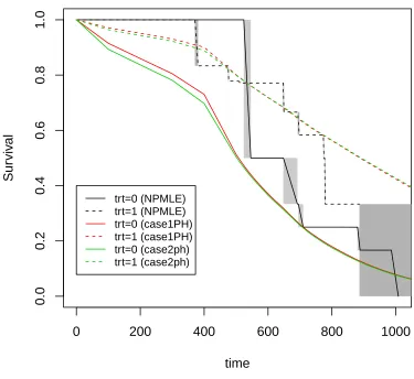
3.5.3 Plot of Survival Functions for the Lung Cancer Data In the input

for both case 1 and case 2 PH models, we used c(0, 1) as the user-specified covariate

vector, which means calculating survival probabilities at grids for treatment = 0

and treatment = 1. Of course, S(t|treatment = 0) = S0(t). Based on the survival

probabilities stored in the ICBayes output element S_m, we can plot the estimated

survival functions for the two treatment groups, using the code shown below. From

Figure 3.6, we can see that the curves from case1PH and case2PH models are not

very close to that from the NPMLE. Actually, the NPMLE is based on Turnbull

(43)

iteration

0 2000 4000 6000 8000 10000

−3.0

−2.5

−2.0

−1.5

−1.0

−0.5

Figure 3.5 Traceplot of the MCMC chain of β in case 2 PH model for lung cancer data

the estimated survival probability before time = 524 days is 1. Similarly, the first

Turnbull interval = (371, 381] for the treatment = 0 group. So the corresponding

estimated survival probability befoer time = 371 is 1. However, our estimates are

smooth rather than step functions, so the estimated survival probabilities during the

two early periods are not going to be constantly 1.

# compared to NPMLE plot

library(interval)

L<-lungdata[,1]; R<-lungdata[,2]; treatment<-lungdata[,4]

R2<-ifelse(is.na(R),Inf,R)

fit1<-icfit(Surv(L,R2,type = ’interval2’)~treatment, data = lungdata)

plot(fit1)

(44)

rect(400,-0.035,800,0.1,col=’white’,border=NA)

legend(0,0.4,c(’trt=0 (NPMLE)’,’trt=1 (NPMLE)’,

’trt=0 (case1PH)’,’trt=1 (case1PH)’,

’trt=0 (case2ph)’,’trt=1 (case2ph)’),

lty=c(1,2,1,2,1,2),col=c(1,1,2,2,3,3),cex=0.8)

0 200 400 600 800 1000

0.0

0.2

0.4

0.6

0.8

1.0

time

Sur

viv

al

treatment=0 treatment=1

trt=0 (NPMLE) trt=1 (NPMLE) trt=0 (case1PH) trt=1 (case1PH) trt=0 (case2ph) trt=1 (case2ph)

(45)

Chapter 4 Modeling Interval-Censored Survival Data with

Spatial Correlation

In randomized clinical trials, subjects are recuited from different geographical regions.

Uncontrolled factors that vary spatially and exert an effect on study outcome may

cause dependency among subjects. Suppose a clinical trial for lung cancer is carried

out in China with patients being recruited from all the provinces. Then from this

mapping of air pollution particles in China (Figure 4.1) , we can see that particle level

varies greatly across the country, and two provinces closer to each other probably have

similar particle level. Since air quality may well affect a person’s lung function, it

suggests that patients may be spatially correlated. Patients from the same province

may be correlated because they share the same air quality, and a province’s air

qual-ity may be affected by its neighboring provinces. In this project, we will model the

described spatial dependency through the conditional autoregressive (CAR)

distri-bution. Furthermore, suppose an endpoint of the trial is progression for lung cancer

patients, then the time-to-event is interval-censored, since progression can only be

examined by CT scan very few weeks.

The conditional autoregressive (CAR) distribution is the most commonly used

model for region-specific random effects. Different from commonly used random

ef-fects that are assumed to be independently and identially distributed, the spatial

random effects are dependent and they jointly follow the CAR distribution. Hodges

Efficient Generation of Power In Medium Voltage Direct Current Systems: Variable Speed Operation and Rectifier Considerations

University of South Carolina

Scholar Commons

Models and Software Development For

Interval-Censored Data

Chun Pan

Acknowledgments

Abstract

Table of Contents

List of Tables

List of Figures

Chapter 1

Introduction

Chapter 2

Background Knowledge

Chapter 3

ICBayes: An R Package for Modeling

Interval-Censored Data

Chapter 4

Modeling Interval-Censored Survival Data with

Spatial Correlation