R E S E A R C H
Open Access
Analysis of the maximum likelihood
channel estimator for OFDM systems in the
presence of unknown interference
Azzouz Dermoune
1*and Eric Pierre Simon
2Abstract
This paper is a theoretical analysis of the maximum likelihood (ML) channel estimator for orthogonal
frequency-division multiplexing (OFDM) systems in the presence of unknown interference. The following theoretical results are presented. Firstly, the uniqueness of the ML solution for practical applications, i.e., when thermal noise is present, is analytically demonstrated when the number of transmitted OFDM symbols is strictly greater than one. The ML solution is then derived from the iterative conditional ML (CML) algorithm. Secondly, it is shown that the channel estimate can be described as an algebraic function whose inputs are the initial value and the means and variances of the received samples. Thirdly, it is theoretically demonstrated that the channel estimator is not biased. The second and the third results are obtained by employing oblique projection theory. Furthermore, these results are confirmed by numerical results.
1 Introduction
Narrow band interference (NBI) arises in orthogonal frequency-division multiplexing (OFDM) systems in a number of transmission scenarios, such as Wi-Fi commu-nications [1, 2] or cognitive radio, where different types of wireless services can use the same frequency band. The NBI can affect several subcarriers. It is well known that it greatly degrades the performance of the receiver if it is not treated [3, 4]. When the transmission is NBI-free, the noise consists only of thermal noise, yielding a uniform noise variance for all subcarriers, resulting in the estima-tion of a single scalar parameter. However, in the presence of NBI, the noise originates from both thermal noise and interference. Due to the nature of NBI, neither the number of affected subcarriers nor their location in the spectrum is known. This brings about the need to estimate the noise variance for each subcarrier, yielding a vector estimation, denotedσ2, rather than a scalar. The objective in the pres-ence of NBI is therefore to estimate the set of parameters
h,σ2, wherehis the vector containing the taps of the channel impulse response.
*Correspondence: [email protected]
1Laboratoire Paul Painlevé, USTL-UMR-CNRS 8524. UFR de Mathématiques, Bât. M2, 59655 Villeneuve d’Ascq Cédex, France
Full list of author information is available at the end of the article
Several methods have been proposed to estimate the channel in the presence of interference. In [5], channel estimation is investigated for OFDM systems in the pres-ence of synchronous interferpres-ence. However, in practical situations, the interferer’s signals are in general asyn-chronous. Zhou et al.’s work [6] deals with the estimation of noise plus interference power together with successive soft data estimation at each subcarrier. Here, we focus on channel estimation based on pilots.
In [7], the authors proposed an estimator employing a specific pilot structure consisting of two types of pilot symbols with different pilot densities. More recently, in [8], a channel estimator is proposed based on a robust least-squares approach. However, the proposed method requires that the number of pilots be greater than twice the channel order, defined as the number of taps.
In [9] and [10], the NBI is assumed to be Gaussian dis-tributed in the frequency domain, with zero mean and unknown power.
Under the same assumptions, channel estimation with NBI is investigated in the seminal paper [11]. The authors also consider the case where any possible correlation between the interference over adjacent subcarriers is neglected. This case can be considered as the worst
case, since correlation is additional information that could be used to improve the estimation. The authors per-form pilot-aided channel estimation under the classical assumption that the number of pilots is greater than the channel order. Note that this assumption is also supposed to be verified in this paper. After formulating the maxi-mum likelihood (ML) algorithm for the joint estimation of h,σ2, it is shown in [11] that the solution is non-unique when the channel order (denoted byL) is greater than the number of transmitted OFDM symbols (denoted by K), leading to ambiguous channel estimates. This is
a severe limitation since K ≤ L is a common scenario
in practice. For example in Wi-Fi scenarios, short frames like control frames are sent frequently. For this reason, the authors suggest resorting to another algorithm, the expectation maximization (EM) algorithm, with the com-plete data set X,σ2, where X contains the received signal. This amounts to treating the noise variances as a nuisance random vector. The drawback of this approach is that it imposes the selection of a distribution for the random vector, the inverse gamma, and then the fixing of the distribution parameter off-line through exhaus-tive grid-search simulations. This can be a limitation for practical use.
In this paper, we first demonstrate that the ambiguities
actually appear only when K = 1 unless the
signal-to-noise ratio (SNR) value is extremely high, in which case ambiguities indeed appear ifK≤L. Thus, for typical SNR values corresponding to practical applications andK >1, the joint ML technique can be used instead of the EM technique. This makes it possible to avoid a grid search.
But even the case K = 1 can be handled with a
spe-cific approach briefly outlined in this paper. Thus, these results open a wider field of application for the joint ML technique.
For the case K > 1, the likelihood equations can be solved with the conditional ML (CML) algorithm. Note that the CML algorithm has been investigated for chan-nel estimation in code division multiple access (CDMA) systems [12]. In this paper, we first present the CML equations for the considered OFDM system. Numerical simulations indicate that the CML is well defined in the SNR range corresponding to practical applications.
Then, we use a new formulation of the CML based on oblique projections to investigate the first moment. Oblique projections are well known for their applica-tions in signal processing, especially in channel estimation [13–16]. With this formulation, it is proved that the chan-nel estimator is unbiased. This result is of importance, in particular, for deriving the Cramer-Rao bound of this channel estimation problem. Moreover, the channel esti-mate is proved to be an algebraic function whose inputs are the initial value and the means and variances of the received samples.
This paper is organized as follows. Section 2 describes the system model. In Section 3, we discuss the joint ML estimation of h,σ2 and the question of the unique-ness of the solution. Then, Section 4 introduces the CML algorithm to find the solution. A theoretical study of the CML is provided in Section 5. The Cramer-Rao bound is derived in Section 6, and simulation results are presented in Section 7.
Notations: The field of complex numbers is denotedC. Matrices [vectors] are denoted with upper [lower] case boldface letters (e.g., Aor a). The complex number ai,j
indicates the (i,j)th entry of the matrix A; ai indicates
the ith entry of the vector a. The vector Ai is the ith
row vector of matrix A. The N × N identity matrix is
denoted by IN, and0M,N is theM×N matrix of zeros.
The matrix D(x) is a diagonal matrix with vector xon its main diagonal. The superscripts (·)T, (·)H, (·)∗, (·)R, and(·)I stand, respectively, for the operations of taking the transpose, Hermitian conjugate, complex conjugate, real part, and imaginary part. The mathematical expec-tation is denotedE[·]. The multivariate complex normal distribution of aP-dimensional random vector is denoted byCN(μ,) whereμis theP-dimensional mean vector andtheP×Pcovariance matrix. The chi-square distri-bution withk degrees of freedom is denoted byχk2. The notations Range(A)and Null(A)indicate, respectively, the range space and the null space ofA.
Note on the notations in bold .2 and |.|2: let a = [a1,· · ·,aN]Tbe a vector of sizeN×1. We use the
nota-tion in bolda2to denote the vector that is formed by tak-ing the square of the entries ofa, i.e.,a2 =[a12,· · ·,a2N]T.
Similarly,|a|2=[|a1|2,· · ·,|aN|2]T.
2 System model
Let us consider an OFDM system with N subcarriers
and a cyclic prefix lengthNg. We assume that the
chan-nel between the transmitter and the receiver is modelled as a frequency-selective fading channel with a
chan-nel impulse response (CIR) vector h of order L, h =
[h1,. . .,hL]T. The CIRhis assumed to be static over the
transmission ofKOFDM symbols. To estimate the
chan-nel,Ppilot symbols with constant energy are inserted into theNsubcarriers at the positionsP = {np,p=1,. . .,P}.
In our paper, we do not consider a particular pilot scheme
P, and all our derivations could be applied to anyP. The only constraint is that L < P. The received frequency-domain pilot sample of thekth OFDM symbol at thenp
subcarrier is
xp,k =cp,kHp+wp,k, (1)
where cp,k is the pilot symbol with normalized power, i.e., |cp,k|2 = 1, transmitted on the n
pth subcarrier,
and wp,k is a disturbance term that takes into account
random complex number wp,k is assumed to be
Gaus-sian distributed with zero mean and unknown variance
σ2
p =σAWGN2 +σNBI,2 p, whereσAWGN2 is the additive white Gaussian noise (AWGN) contribution and σNBI,2 p is the average NBI power, which is assumed constant over the transmission period. The channel frequency responseHp
at thenpth subcarrier is given by
Hp=
This yields the model for thePpilot subcarriers of the kth received OFDM block:
xk=CkFh+wk, k=1,. . .,K, (3)
withxk =[x1,k,. . .,xP,k]T,wk =[w1,k,. . .,wP,k]T,Ck =
D([c1,k,. . .,cP,k]), where D(u) is the diagonal matrix
with the entries of vector u on its diagonal and F is
the P × L matrix with the (p,l)th entry defined as
The ML estimation of the set of unknown parameters {h,σ2}is desired, whereσ2= σ12,. . .,σP2T, based on the set of received samples{yk =C−k1xk,k=1,. . .,K}.
Let us now define the sample means and the sample variances of the received samples, which will be used in the rest of the paper. The sample mean vector is denoted byy¯=[¯y1,. . .,y¯P]T, where forp=1,. . .,P,
The sample variance vector is denoted by s2 =
s21,. . .,s2PT, where forp=1,. . .,P,
3 Maximum likelihood estimation
In this section, the ML estimate of{h,σ2}will be investi-gated by following the approach presented in [11]. How-ever, it will be shown that the ambiguities mentioned in
[11] appear only whenK = 1, unless the SNR value is
extremely high. Hence, whenK ≥ 2 and practical SNR
values are considered, it will be possible to get the ML
solution without ambiguities. The estimates whenK ≥
2 will be derived through the conditional ML and their properties studied in the next section.
Recall that theK independent observationsy1,. . .,yK
are drawn from the followingp-variate normal regression model:
The approach to derive the ML solution is summed up below. The variances which minimize (7) for a givenh˜are first calculated:
Finally, the ML estimate of the CIR vectorhis the one that minimizes(h˜). Special treatment is required due to the presence of the logarithm function in (9). Indeed, the values ofh˜for whichσˆp2(h˜)= 0 make(h˜)tend to−∞. The consequences for the uniqueness of the solution are explained in more detail in [11], where it is shown that the minimization leads to ambiguous channel estimates if K ≤ L. At this point, it is important to precise the con-text leading to this result. It was assumed that no prior knowledge about the noise variances was available, which implied that theoretically they could be zero. However, in practice, the noise variance is never zero due to the pres-ence of thermal noise. We will now revisit this ambiguity issue by taking into account the fact that the noise vari-ance is not zero. Let us first observe that the equation
ˆ σ2
p(h˜) = 0 (8) for a givenpyields a linear system ofK
equations withLunknowns:
Ah˜ = yp,1,. . .,yp,K T
, (10)
where the K ×L matrix Ais built by stacking the row
vectorsFp. IfK = 1, then the system (10) is
underdeter-mined (one equation andLunknowns), yielding an infinite number of solutions. However, forK > 1, the specific structure ofAhas to be taken into account when solv-ing the system. On the one hand, the rows of Aare all identical. On the other hand, in the presence of AWGN, the samplesyp,1,. . .,yp,K are all different since they are
conditioned if the SNR is less than 150 dB, which is the case of practical applications.
This ambiguity issue appears more clearly with the formulation of σˆp2(h˜) based on the sample means and
This article is concerned with the case K > 1. How-ever, it is worth mentioning that the case of K = 1 can still be handled with the following approach. It has been shown that it is meaningless to search for the ML ofσ2in the domain(0,+∞)P. A possible solution is to restrict the parameter space by imposing a priori lower bounds of the form [17]
minimize (7) for givenh˜are given by
ˆ
and then the CIR estimatehˆ is the one that minimizes
(h˜,δ2)with respect toh˜.
As previously stated, this article will focus onK > 1. As there is no closed-form solution for the minimiza-tion of(h˜), we suggest using the conditional ML in the next section to find an iterative solution and study the properties of this solution.
4 Conditional ML
The CML algorithm is an iterative algorithm for solving the ML problem. The CML is the result of two nested minimiza-tions. First, (7) is minimized given the channelh˜, yielding the estimation ofσ2given by (8) or (11):
section). Conversely, (7) is minimized givenσ˜2, yielding the following estimate forh:
ˆ
We obtain the following iterative algorithm, withI the number of iterations:
We recall that we have used the notations in bold defined in the notation section. Note that with this ini-tialization, hˆ(1) is the ordinary least-squares estimate of h. Note also that the expectation-maximization algo-rithm of [11, equations (28),(29)] corresponds to the CML algorithm forλ=0.
This algorithm is known as the scoring method [18, 19] or the conditional maximum likelihood (CML) algorithm [20].
The CML’s important properties include:
1. Given σˆ2(i), the vector hˆ(i+1) maximizes the
likeli-converges to some constant
ln(c∗)≥Pp=1lns2p.
In this section, the CML algorithm has been presented with some of its well-known properties. However, to our knowledge, no work has been carried out about the moments of the CML solution in this particular context. The next section will address this topic.
5 Theoretical analysis of the CML algorithm
In this section, some properties of the CML algorithm are studied. In particular, the first moment of the estimators is investigated. To do so, a formulation of the CML based on oblique projections is established. It will be shown that the CML algorithm can be viewed as successive oblique projections.
5.1 The CML algorithm and oblique projections
( ) := F(FH F)−1FH splits the spaceCP into two
subspaces: the range space Range(( ))=( )CPof
( )and its null space Null(( )) =[I−( )]CP. Note that the range of( )is the range ofF. The linear operator defined by( )is known as an oblique projec-tion onto Range(F). If =I, then(I)= FFHF−1FH is the orthogonal projection on Range(F). For simplicity of notation,(I)is now denoted by.
Now, we go back to the CML algorithm defined in the previous Section.
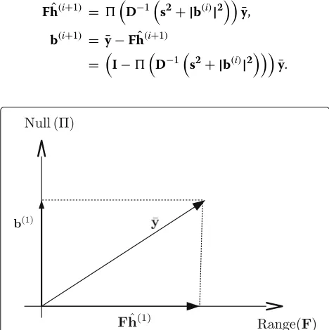
At the first iteration, the orthogonal projectionsplits the sample mean into the following two components (see Fig. 1 for a geometrical interpretation):
Fhˆ(1) = y¯,
b(1) := (I−)y¯. (19)
The vectorb(1) is the orthogonal projection ofy¯ onto Null().
Givenhˆ(1), the ML of the variance vector is given by
ˆ
σ2(1)=s2+|b(1)|2,
where the column vector|b(1)|2=
|b(1)
1 |2,. . .,|b
(1)
P |2 T
. At thei+1th iteration, we have
ˆ
h(i+1)=FHD−1s2+|b(i)|2F−1
FHD−1
s2+|b(i)|2
¯ y.
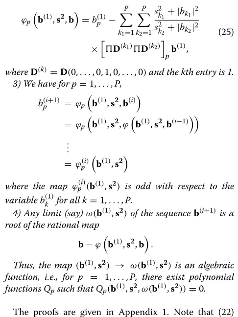
The oblique projectionD−1s2+|b(i)|2splits the sample mean into the following two components (see Fig. 2):
Fhˆ(i+1) = D−1s2+|b(i)|2y¯,
b(i+1) = ¯y−Fhˆ(i+1) = I−
D−1
s2+|b(i)|2
¯ y.
Fig. 1First iteration of the CML algorithm: orthogonal projection
Fig. 2Iterationi≥1 of the CML algorithm: oblique projection
Givenhˆ(i+1), the ML of the variance vector is given by
ˆ
σ2(i+1)=s2+| b(i+1)|2.
From this discussion, it can be concluded that the solu-tion provided by the CML algorithm can be sought either inFhˆ(i)or in the variableb(i)= ¯y−Fhˆ(i). In the
perspec-tive of investigating the CML properties, it will be seen that it is more convenient to considerb(i), which yields an equivalent algorithm for solving the CML:
b(i+1)=(I−
D−1
s2+|b(i)|2
¯
y. (20)
Now, let us study the properties of Eq. (20). To do so, let us first writeb(i+1)as a function of the three following variablesb(i+1)=ϕy¯,s2,b(i)where
ϕy¯,s2,b(i)
:=(I−
D−1
s2+|b(i)|2
¯ y, (21)
is a function of sizeP×1. From now on,ϕpdenotes the
pth entry ofϕ. Now, the following properties are stated in Proposition 1. They will be used to derive Proposition 2.
Proposition 11) For i≥1,
ϕy¯,s2,b(i)
=ϕb(1),s2,b(i)
, (22)
and
ϕb(1),s2,b(i)
=I−D
s2+|b(i)|2
× D−1
s2+|b(i)|2
b(1).
(23)
2) The maps
ϕpb(1),s2,b
=I−Ds2+|b|2D−1s2+|b|2pb(1) (24)
Recall that the subscript p applied to a matrix means taking the pth row of the matrix. More precisely,
ϕp
root of the rational map
b−ϕb(1),s2,b.
Thus, the map(b(1),s2) → ω(b(1),s2)is an algebraic function, i.e., for p = 1,. . .,P, there exist polynomial functions Qpsuch that Qp(b(1),s2,ω(b(1),s2))=0.
The proofs are given in Appendix 1. Note that (22) is straightforward with the geometrical interpretation of Fig. 2, where it can be observed that the projections ofb(1) andy¯onto NullD−1(s2+|b(i)|2)are the same.
5.2 The mean of the CML estimator
The distributions of the sample mean and the sample vari-ance are derived in Appendix 2. Upon the convergence of the algorithm (20), we obtain hˆ, bˆ, and σˆ2. FromFhˆ =
using the property that the mean of a chi-square random variable ofndegrees of freedom isn. Now, from Proposi-tion 1, the following can be shown (see Appendix 3 for the proof ).
Proposition 2 The vectorbˆis zero mean, i.e.,
Ebˆp
=0, p=1,. . .,P. (28)
Therefore, from (26),hˆis an unbiased estimator.
5.3 Complexity of the CML algorithm
In this Section, the complexity of the CML algorithm (20) is investigated. First, it is noteworthy that it is more interesting in terms of complexity to use the formulation (23) instead of (20). Indeed, in (20), the matrix inversion
FH(D−1s2+|b(i)|2F−1 is required at each iteration, whereas in (23), the computation of matrixcan be done off-line and stored in a memory. In this way, the opera-tions for computing (23) only consist in matrix products, which is less demanding. Moreover, the calculation ofs2 is carried out just once at the beginning of the algorithm. Therefore, the algorithm requires O(P3) floating point operations in total for each iterationi.
6 The Cramer-Rao bound
Let us define the 2L+P×1 vector of the real parameters to be estimated:
θ = hR1,. . .,hRL,hI1,. . .,hIL,σ12,. . .,σP2T, (29)
wherehRl,hIl are, respectively, the real and imaginary parts ofhl.
The Cramer-Rao bound (CRB) for this estimation prob-lem states that the covariance matrix ofθˆsatisfies
cov(θˆ)≥ ∂ψ(θ) lated by assuming perfect knowledge of the variance. In this Section, both channel and variance parameters are being considered. The matrixJ is the 2L+P×2L+P Fisher information matrix. Its (m,n)th entry is defined asE∂θ∂2
n∂θm
h,σ2, where(h,σ2)is the negative log-likelihood defined in (7).
Therefore, it can be seen from (31) that knowing the moments of the estimator is required in order to calculate the CRB. The results of Section 5.2 will be exploited to do so.
The results of the calculation of J are given below, and the details are in Appendix 4. The matrix Jcan be written as
and where the entries of
Jh are defined by (41), (42), and (43) in Appendix 4. To
the block diagonal matrix of the inverses of the blocks, as long as the submatrices are invertible, we have
J−1=
J−h1 02L,P
0P,2L J−σ21
. (33)
From (26), (27), and Proposition 2, we can expressψ(θ) as a function ofhandσ2and calculate the derivative:
∂ψ(θ) ∂θ =
I2L 02L×P
0P×2L M
(34)
where the(p1,p2)th entry of Mis defined as KK−1δpp12 +
E
∂|ˆbp1|2
∂σ2
p2
. Therefore, we have
∂ψ(θ) ∂θ J−1
∂ψ(θ) ∂θ
T
=
J−h1 02L×P
0P×2L MJ−σ21MT
. (35)
Note that the calculation of E
∂|ˆbp1|2
∂σ2
p2
is not feasible
since there is no analytical expression forbˆ. Therefore, the bound for the variance estimation cannot be found. How-ever, the bound for the channel estimation is given from (29) and (35) by
cov
ˆ
hR1,. . .,hˆRL,hˆI1,. . .,hˆILT
≥J−h1. (36)
Recall that this bound has been derived by using the result of Proposition 2 showing thathˆwas unbiased.
7 Simulation results
In order to validate the results, computer simulations were carried out in accordance with the IEEE 802.11g standard, with a carrier frequency equal to 2.4 GHz. The system parameters used for the simulation are as follows:N =64 subcarriers, a bandwidth of 20 MHz, and a cyclic prefix of length 16. The discrete-time channel is assumed to have
L = 6 channel taps modelled with a Rayleigh channel
with an exponentially decaying power such thatE[|hl|2]= σ2
h ·exp(−l)withl = 1, 2,· · ·,L = 6. The constantσh2
is chosen to normalize the channel power to one. For the simulation, the pilots are evenly inserted every eight sub-carriers, yieldingP=8. A frame ofK=4 OFDM symbols is assumed. Note thatK<Lwith these considered values. It is also assumed that two contiguous pilot subcarri-ers are affected by NBI, by adding a Gaussian disturbance of varianceσNBI2 to both subcarriers. The signal-to-noise ratio (SNR) is defined as 10 logσ21
AWGN
where the power of the signal is normalized to one, and the signal-to-interference ratio (SIR) is defined as 10 logσ12
NBI
. The accuracy of the channel estimates is measured in terms of the mean square error (MSE), which is defined as
1
LE
(hˆ−h)H(hˆ−h), where the expectation is esti-mated via Monte Carlo simulations.
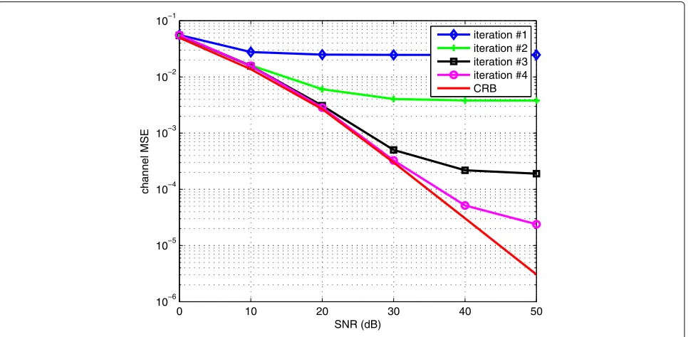
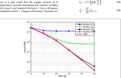
Figure 3 shows the MSE as a function of the SNR when the SIR is fixed to−5 dB. Four iterations are employed. Let us recall that the first iteration is the ordinary least-squares estimate (OLSE). For reference, the CRB calcu-lated in Section 6 is added. It is seen that the algorithm converges after four iterations for the SNR ranging from 0
0 10 20 30 40 50
10−6 10−5 10−4 10−3 10−2 10−1
SNR (dB)
channel MSE
iteration #1 iteration #2 iteration #3 iteration #4 CRB
to 30 dB and nearly attains the CRB, whereas the MSE for the OLSE has a floor at 2.5×10⁻². This shows that the ML algorithm is well conditioned for the considered SNR range [ 0, 50] dB.
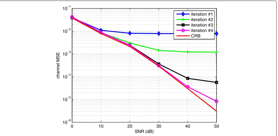
Next, the SIR is fixed to 0 dB in Fig. 4 and to 5 dB in Fig. 5. In these two cases, the algorithm converges after only three iterations. Moreover, it can be observed that the performance of the OLSE approaches that of the second iteration when the SIR increases. This makes sense, as the OLSE is designed to perform well without NBI.
To investigate the impact of the number of OFDM sym-bols on the performance,Kis now fixed to 8 and the other parameters are the same. The results are shown in Fig. 6
for an SIR = −5 dB. Compared to K = 4, it can be
observed that the convergence is faster, since only three iterations are needed to converge. This is understood since it is a more favorable scenario (Fig. 6).
Finally, the bias ofhˆ is studied. We plot the histogram of the real part and imaginary part ofbˆp,p = 1,. . .,Pin
Figs. 7 and 8, respectively. The SNR is fixed to 10 dB and the SIR to 0 dB. It can be observed that the mean is zero for allp, which leads to an unbiased estimator forhˆ. This confirms Proposition 2).
8 Conclusions
This article has addressed the problem of maximum like-lihood channel estimation for OFDM systems in the pres-ence of unknown interferpres-ence. First, it was proved that the solution is without ambiguities as long as the num-ber of transmitted OFDM symbols is strictly greater than one. For this case, we proposed using the conditional
maximum likelihood (CML) algorithm to obtain the esti-mates. New theoretical developments of the CML algo-rithm in this context have been presented. It was proved that the solution provided by the CML is an algebraic function of the data. Furthermore, it was also proved that the channel estimator is unbiased.
Appendix 1: Proof of Proposition 1
The proof of Proposition 1 1) is a consequence of the fol-lowing general results. We have for any invertible matrix
that
(I−( ))=(I−( ))(I−).
The latter equality is equivalent to
=( ).
Now, it can be easily shown that
( )=FFH F−1FH FFHF−1FH=.
The proof of 2) is a consequence of the following general result:
FH −1F−1=F+ FH+
whereF+= FHF−1FH andFH+= FFHF−1. From this, we have
−1=FF+ FH+FH −1= −1. (37)
The proof of the remaining assertions is straightforward.
0 10 20 30 40 50
10−6 10−5 10−4 10−3 10−2 10−1
SNR (dB)
channel MSE
iteration #1 iteration #2 iteration #3 iteration #4 CRB
0 10 20 30 40 50 10−6
10−5 10−4 10−3 10−2 10−1
SNR (dB)
channel MSE
iteration #1 iteration #2 iteration #3 iteration #4 CRB
Fig. 5Performance of the CML estimator as a function of the SNR for SIR=5 dB,K=4
Appendix 2: Probability distribution function of the sample mean and the sample variance
Cochran’s theorem [21] states that the sample mean and variance are two independent random variables.
More-over, it is also stated that the sample variance of K
independent normally distributed real random variables with mean 0 and standard deviation 1 has a chi-square distribution withK−1 degrees of freedom. Therefore, we
can write down the distribution fors2p. The distribution fory¯pis straightforward:
¯
yp ∼ CN
Fph, σ2
p
K
, (38)
s2p ∼ σ
2
p
2Kχ
2
2(K−1). (39)
0 10 20 30 40 50
10−6 10−5 10−4 10−3 10−2 10−1
SNR (dB)
channel MSE
iteration #1 iteration #2 iteration #3 iteration #4 CRB
Fig. 7Histogram ofbˆR
p,p=1,. . .,P, SNR = 10 dB, SIR = 0 dB
Here we find 2(K − 1) degrees of freedom since the
considered random variables are complex.
Appendix 3: Proof of Proposition 2
The Gaussian vector b(1), defined in (19), is zero mean with the covariance matrix K−1(I−)D(σ2), i.e., (I− )y¯∼(I−)K−1/2D(σ)N(0,I).
The components of the vector 2Ks2 are independent
with the distribution σ12χ22(K−1)(1),. . .,σP2χ22(K−1)(P).
Here χ22(K−1)(1),. . .,χ22(K−1)(P) are i.i.d. with the com-mon distribution χ22(K−1). From Cochran’s theorem, s2 andy¯ are independent. From Proposition 1, the random vectorb(i+1) =ϕ(i)b(1),s2is a rational function having a positive denominator. Therefore,
Eb(i+1)|s2
because b(1) is zero mean which implies that its prob-ability density function b → fb(1)(b) is even and b → ϕ(i)(b,s2) is odd. Then, using the basic property
E(E(X|Y))=E(X), whereXandYare random variables, we obtain (28).
Appendix 4: The Fisher information matrix
To facilitate the calculations, the negative log-likelihood is rewritten using real numbers:
∂2
Now, the expectation needs to be taken to findJ. The expectations of (41), (42), and (43) are unchanged. From the definition ofbp= ¯yp−Hpand (38), the expectation of
This works has been carried out in the framework of The ELSAT2020 project which is co-financed by the European Union with the European Regional Development Fund, the French state, and the Hauts de France Region Council. This work has been supported in part (or partially) by IRCICA USR 3380 CNRS-Univ (project: connected objects ) , F-59000 Lille, France (hppt://www. ircica.univ-lille1.fr).
Funding
We confirm that we do not have a funding source.
Authors’ contributions
AD and EPS both worked on the calculation of the theoretical results. EPS made the matlab programs. Both authors read and approved the final manuscript.
Competing interests
The authors declare that they have no competing interests.
Publisher’s Note
Springer Nature remains neutral with regard to jurisdictional claims in published maps and institutional affiliations.
Author details
1Laboratoire Paul Painlevé, USTL-UMR-CNRS 8524. UFR de Mathématiques,
Bât. M2, 59655 Villeneuve d’Ascq Cédex, France.2IEMN lab, TELICE group, University of Lille, Lille, France.
Received: 8 February 2017 Accepted: 19 September 2017
References
1. K Ohno, T Ikegami, Interference mitigation technique for coexistence of pulse-based UWB and OFDM. EURASIP J.Wirel. Commun. Netw.2008(1), 285683 (2008)
2. J-W van Bloem, R Schiphorst, T Kluwer, C Slump, inWireless
Communications, Networking and Mobile Computing (WiCOM), 2012 8th International Conference on. Interference measurements in IEEE 802.11 communication links due to different types of interference sources, (Shangai, 2012), pp. 1–6
3. A Coulson, Narrowband interference in pilot symbol assisted OFDM systems. IEETrans, E,Wireless Commun.3(6), 2277–2287 (2004) 4. AJ Coulson, Bit error rate performance of OFDM in narrowband
interference with excision filtering. IEEE Trans Wireless Commun.5(9), 2484–2492 (2006)
5. A Jeremic, T Thomas, A Nehorai, OFDM channel estimation in the presence of interference. IEEE Trans. Signal Process.52(12), 3429–3439 (2004)
6. J Zhou, J Qin, Y-C Wu, Variational inference-based joint interference mitigation and OFDM equalization under high mobility. IEESignal Signal Process. Lett.22(11), 1970–1974 (2015)
7. S Lee, K Kwak, J Kim, D Hong, Channel estimation approach with variable pilot density to mitigate interference over time-selective cellular OFDM systems. IEEE Trans. Wireless Commun.7(7), 2694–2704 (2008) 8. Y Zhang, X Zhang, D Yang, inWireless Communications and Networking
Conference (WCNC), 2013 IEEE. A robust least square channel estimation algorithm for OFDM systems under interferences, (Shangai, 2013), pp. 3122–3127
9. T Li, W-H Mow, V Lau, M Siu, R Cheng, R Murch, Robust joint interference detection and decoding for OFDM-based cognitive radio systems with unknown interference. IEEE J.Sel. Areas Commun.25(3), 566–575 (2007) 10. M Morelli, M Moretti, Robust frequency synchronization for OFDM-based cogni
tive radio systems. IEEE Trans. Wireless Commun.7(12), 5346–5355 (2008) 11. M Morelli, M Moretti, Channel estimation in OFDM systems with unknown
interference. IEEE Trans. Wireless Commun.8(10), 5338–5347 (2009) 12. X Mestre, JR Fonollosa, ML approaches to channel estimation for
pilot-aided multirate DS/CDMA systems. IEEE Trans. Signal Process.50(3), 696–709 (2002)
13. RT Behrens, LL Scharf, Signal processing applications of oblique projection operators. IEEE Trans. Signal Process.42(6), 1413–1424 (1994) 14. RT Behrens, LL Scharf, Corrections to “signal processing applications of
oblique projection operators” [correspondence]. IEEE Trans. Signal Process.44(5) (1300)
15. B Cao, Q-Y Zhang, L Jin, N-T Zhang, Oblique projection polarization filtering-based interference suppressions for radar sensor networks. EURASIP J. Wirel. Commun. Netw.2010(1), 605103 (2010)
16. W Qiu, SK Saleem, E Skafidas, Identification of MIMO systems with sparse transfer function coefficients. EURASIPJ.Adv. Signal Process.2012(1), 104 (2012) 17. H Hartley, K Jayatillake, Estimation for linear models with unequal
variances. J. Am. Stat. Assoc.68(341), 189–192 (1973)
18. EB Andersen, Asymptotic properties of conditional maximum-likelihood estimators. J. R. Stat. Soc. Ser. B Methodol. 283–301 (1970)
19. TH Szatrowski, Necessary and sufficient condition for explicit solutions in the multivariate normal estimation problem for patterned means and covariances. Ann. Stat.8, 802–810 (1980)
20. AP Dempster, NM Laird, DB Rubin, Maximum likelihood from incomplete data via the EM algorithm. J. R. Stat. Soc. Ser. B Methodol. 1–38 (1977) 21. WG Cochran, inMathematical Proceedings of the Cambridge Philosophical