RELIABILITY EVALUATION OF MULTIPLE
PERFORMANCE PARAMETERS SYSTEM ADT BASED ON
MULTIDIMENSIONAL TIME SERIES MODEL
1LI WANG, 2ZAIWEN LIU, 2CHONGCHONG YU 1
Dr., School of Computer & Information Engineering, Beijing Technology & Business University, China
2Prof., School of Computer & Information Engineering, Beijing Technology & Business University, China
E-mail: [email protected]
ABSTRACT
This paper proposes a new Accelerated Degradation Testing (ADT) reliability evaluation method utilizing a multidimensional composite time series modeling procedure to take into account the integrated effect of system’s multiple performance parameters along with the random effect of environmental variables for equivalent damage in ADT. In this paper, system performance parameter ADT data are treated as a multidimensional composite time series model to predict system failure time. First, this paper decomposes these multiple performance parameters useful for ADT into three classes as trend, cyclical or random components, and describes them with a combined multi-dependent variable regressive model, hidden periodic model and multivariate auto-regression model. Second, according to standard practice, this paper assumes that the failure of such a system obeys a competing failure rule, that is, for an individual unit there is one primary controlling variable that will indicate failure even though others degrade they do not meet any failure criterion. Failure time at each test-stress level is predicted by using the best linear unbiased prediction of the multidimensional composite time series model. Finally, the reliability at use-stress level is estimated from a failure time distribution evaluation based on the failure time predictions at each test-stress level providing a relationship between failure time and test-stress levels.
Keywords: ADT, Multidimensional Time Series, Reliability Evaluation, Multiple Performance Parameters 1. INTRODUCTION
For long lifetime and high reliability products or systems, it is difficult to obtain failure data in a short time period. Hence, Accelerated Degradation Testing (ADT) is presented to deal with the cases where no failure time data could be obtained but degradation data of parameters of the system are available. At present, the ADT reliability evaluation method is utilized primarily with feedback from a single performance parameter system ADT dataset. However, for most systems, multiple performance parameters of these systems will degrade with time, leading to failure. It is important to note that often the systems various performance parameters will interact with each other as the performance degrades. Hence, a correct reliability evaluation based on ADT data must take into account the
integrated effect of a system’s multiple
performance parameters and the random effect of environmental variables.
In the literature, such as in the noted references [1-5], ADT reliability evaluation is studied using time series methods due to its excellent capability of stochastic and periodic information mining. However, reliability evaluations using the time series method in present literature are all based upon a one-dimensional time series analysis. To take into account multiple dimensions of system performance degradation, it is important to study these parameters using an ADT reliability evaluation based on a multidimensional time series analysis method.
2. MULTIDIMENSIONAL TIME SERIES MODELING
The stochastic analysis for multiple performance parameters degradation data with multidimensional time series analysis is based on the following hypotheses:
(1) All performance parameters of a system
degrade monotonically;
the same during the degradation process;
(3) The data collection for all parameters is
concurrent.
In ADT, performance degradation data is usually collected at defined consistent intervals producing a homogeneous variance. Typically, degradation data is not stationary per hypothesis (1) above.
Let Yt denotes the multiple performance
parameters degradation measurement at time t.
Based on the Cramer Decomposition Theorem, any
multidimensional time series {Yt} can be
decomposed into three components: a deterministic component, a cyclical component and a stationary
random component. Hence, Yt could be expressed
as,
1 1 1 1
2 2 2 2
,
1, 2,
,
,
,
,
t t t t
t t t t
t t t t
t t t t
nt nt nt nt
t
N
y
d
c
r
y
d
c
r
y
d
c
r
=
+
+
=
=
=
=
=
Y
D
C
R
Y
D
C
R
(1)
Here Dt is multidimensional deterministic
component. Ct is multidimensional cyclical
component. Rt is the multidimensional stationary
random component,
y
it is a degradationmeasurement of ith performance parameter,
d
itis thedeterministic component of ith performance
parameter,
c
it is a the cyclical component of ithperformance parameter,
r
itis the stationary randomcomponent of ith performance parameter, i=1,2,…
,n, where n is the total number of performance
parameters and N is total sampling time.
2.1 Multidimensional deterministic component modeling
The multidimensional deterministic component
Dt is extracted from the performance degradation
data using a multi-dependent variable regression model,
( )
( )
( )
( )
1 01 01 1
2 02 02 2
0 0
1 t
n n n n
b g t y y b
b g t y y b
g t
b g t y y b
+
+
= =
+
D
(2)
Here D(t) is a n-dependent variable regression
function which effectively fits the degradation trend
of the data, bi is the degradation rate of ith
performance parameter, g(t) is a monotonic
regression function, y0i is the initial value of the ith
performance parameter, i=1,2,…,n.
2.2 Multidimensional cyclical component modeling
The multidimensional deterministic component
Dt is extracted from multiple performance
parameters. Then the multidimensional cyclical
component Ct, is modeled using Hidden Periodic
model,
1
2
1 1 1
1 1
2 2 2
2
1
1
cos(
)
cos(
)
cos(
)
nk
j j j
j
t k
j j j
t j t
nt k
nj nj nj
j
a
t
c
a
t
c
c
a
t
ω
j
ω
j
ω
j
=
=
=
+
+
=
=
+
∑
∑
∑
C
(3)
Here aij is the amplitude of i
th
performance
parameter,
k
i is the ith
total number of angular
frequency,
ω
ij is the jth angular frequency,
φ
ij is thejth phase, i=1,2,…,n.
2.3 Multidimensional random component modeling
The multidimensional cyclical component Ct is
extracted from multiple performance parameters.
Then the multidimensional random component Rt,
is modeled using a multidimensional autoregressive model,
1
11 12 1 1
21 22 2 2
1 2
,
,
pt j t j t
j
j j nj t
j j nj t
j t
n j n j nnj nt
η
η
η
ε
η
η
η
ε
η
η
η
ε
− =
=
+
=
=
∑
R
Η R
Ε
Η
Ε
(4)
Here p is the order of multidimensional
autoregressive model; Hjis a n×n multidimensional
autoregressive coefficient matrix. çikj is the ith
performance parameter multidimensional
autoregressive coefficient from kth performance
parameter, Etis a n-dimensional white noise vector
which obeys
N
[0,
Q
]
, åit is the white noise of ith2.4 Multiple performance parameters degradation modeling
The multi-dependent variable regression model
for the deterministic component Dt, the hidden
periodic model for the cyclical component Ct and
the AR model of the stationary random component
Rt are combined into Yt. Hence, the performance
degradation measurement Yt is obtained as,
1 p
t t t t t t j t j t
j
− =
=
+
+
=
+
+
∑
+
Y
D
C
R
D
C
Η R
Ε
(5)It can also be expressed as,
( )
12
1 1 1
1 01 1
1
02 2 2 2 2
2
1
0
1
11 12 1
21 22 2
1 2
cos( )
1 cos( )
cos( )
n
k
j j j
j
t k
j j j
t
j
n n
nt k
nj nj nj
j
j j nj
j j nj
n j n j nnj
a t
y b y
y b a t
y g t y b y a t
ω
j
ω
j
ω
j
η
η
η
η
η
η
η
η
η
= = = + + = + + +
∑
∑
∑
( ) ( ) ( ) 1 1 2 2 1 t j t pt j t
j
nt n t j
r r r
ε
ε
ε
− − = − + ∑
(6) Eq.5 is called multidimensional Regression-Auto Regression (RAR) model in this paper.
3. MULTIDIMENSIONAL RAR MODEL PARAMETERS ESTIMATION
3.1 Deterministic component model parameters estimation
Parameters for the multi-dependent variable regression model are estimated using a Least-Square estimation method. Its principle is to
minimize the sum of quadratic sum of Rt, which is
2 1 1 N n R it t i
r
= ==
∑∑
Q
Let 11 1 1 N n nN y y y y = Y ,
g
=
(
g
( ) ( )
1 ,
g
2 ,
,
g N
( )
)
(
)
0 01 02 0
ˆ
=
y
ˆ
,
y
ˆ
,
,
y
ˆ
n Ty
,b
ˆ
=
(
b b
ˆ ˆ
1,
2,
,
b
ˆ
n)
TThe regression coefficient is estimated by using the matrix inversion formula. That is
1 0 1
ˆ
ˆ
T T gg gy T gg gy − −
−
=
y
Y
gL L
L L
b
Here
1 T T gg
n
= −
L g I 1 1 g , 1 T T gy
n
= −
L g I 1 1 Y ,
1
n
=
g g, 1 T n
=
Y Y1 ,1=
(
1,1,,1)
, 1 00 1 = I
3.2 Random component model parameters estimation
Parameters of the multidimensional autoregressive model are estimated by a Yule-Walker estimation method.
Point estimation of mean value of Rt, which
isμ=ERt, is
(
1 2)
1
1 ˆ ˆ ,ˆ , ,ˆ
N T
N n t
t N =
= =
∑
μ μ μ μ R (7)
The estimate of the autocovariance function Γ
( )
his
( )
(
)(
)
( )
( )
11
ˆ ˆ ˆ , 0 1
ˆ ˆ , 1 1 N h
T t h N t N t
T
h h N
N
h h h N
− + = = − − ≤ ≤ − − = ≤ ≤ −
∑
Γ R μ R μ
Γ Γ
(8) Thus the Yule-Walker equation is
( )
( )
( )
(
)
1 1
ˆ ˆ 0 ˆ ˆ
ˆ ˆ ˆ , 1
p j j p j j j
h h j h
= = = − + − = − ≥
∑
∑
Γ HΓ Q
Γ HΓ
(9) Then ( ) ( ) ( ) ( ) ( ) ( ) ( ) ( ) ( ) ( ) ( ) ( )
ˆ 1 ˆ 0 ˆ 1 ˆ 1
ˆ 2 ˆ 1 ˆ 0 ˆ 2
ˆ ˆ 1 ˆ 2 ˆ 0
T
T
T
p
p
p p p
− = − − − + − +
Γ Γ Γ Γ
Γ Γ Γ Γ
Γ Γ Γ Γ
1 2 ˆ ˆ ˆ T T T p H H H (10)
The autoregressive coefficient,
(
H Hˆ1, ˆ2,,H Qˆp,ˆ)
,
is estimated by solving Yule-Walker equation.
4. RELIABILITY EVALUATION & ACCELERATED MODELING
reliability evaluation for the system at use-stress level is obtained by failure time distribution of systems, reliability evaluation at each test-stress level and accelerated modeling.
4.1 Multiple performance parameters degradation prediction
The
l
th step prediction of Yt is obtained fromthe best linear unbiased prediction of Eq.4. The prediction formula is
1
N l N l N l N l
p
N l N l j N l j
j
+ + + +
+ + + −
=
=
+
+
=
+
+
∑
Y
D
C
R
D
C
Η R
(11)4.2 Failure time prediction
In practice, the failure of systems having multiple performance parameters usually obeys the competing failure rule. That is, for most of these systems, they will degrade with time where the specific performance parameter that first passes a specified failure threshold for an individual unit will lead to the failure of that unit.
Hence, according to the competing failure rule,
when total number of performance parameters is n,
this paper sets failure threshold respectively, which
is
(
D D
1,
2, ,
D
n)
, for each performance parameterof the system. The failure time of each performance
parameter, which is
(
)
1
,
2,
,
nD D D
t
t
t
, is the timethat each performance parameter passes its own
failure threshold
(
D D
1,
2, ,
D
n)
. This is predictedby Eq.10. The reliability evaluation of the system then is the minimum failure time prediction of all performance parameters,
(
1 2)
min , , ,n
f D D D
t = t t t
(12)
4.3 Failure time distribution
The reliability evaluation is assumed to obey a certain location-scale distribution as determined by a Pearson chi-square Goodness of Fit Test. The estimate of the location and scale parameters of the failure time distribution are obtained by MLE. This
paper denotes reliability evaluation of ith system
as
t
f i( ), when total number of systems is m, andthen the prediction of the maximum likelihood function for the distribution of failure time is
( )
(
( ))
1
,
mf i i
L
β
f t
β
=
=
∏
(13)Here,
(
,)
Tβ= µ σ , T means transpose of matrix.
4.4 Accelerated modeling
To obtain the ADT reliability evaluation for the at use-stress level, it is necessary to convert the reliability evaluation at each test-stress level to the equivalent reliability evaluation at the use-stress level. This paper converts the reliability evaluation of systems from each test-stress level into a reliability evaluation for the system at its’ use-stress level based on the stress level-median failure time relationship and accelerated model
( )
a b
S
µ
= +
j
(14)
Here, μ is median failure time at each test-stress
level; S is test-stress level; a, b are parameters
estimated from degradation data. φ(S) is a known
function of S.
5. ADT DATA VERIFICATION
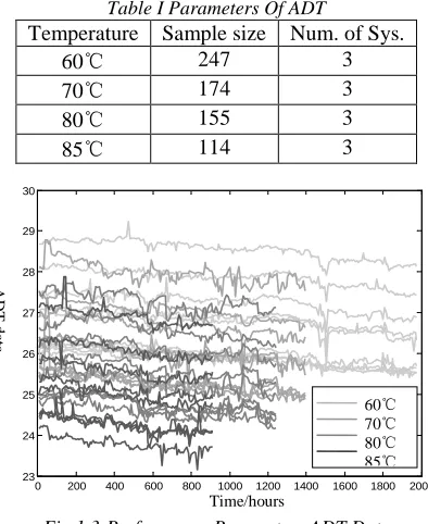
[image:4.612.318.515.415.656.2]The four temperature stress levels ADT were processed for a certain microwave electronic system to verify the multidimensional time series analysis method. The personal computer records 3 different performance parameters of each test unit every 8 hours. Table I shows the temperature test parameters. The multiple performance parameters degradation path for each system is shown in Fig.1.
Table I Parameters Of ADT
Temperature Sample size Num. of Sys.
60℃ 247 3
70℃ 174 3
80℃ 155 3
85℃ 114 3
Fig.1 3-Performance Parameters ADT Data
The ADT data of each unit is preprocessed to normalize for the initial performance value to minimize sample bias. Fig.2 shows them.
0 200 400 600 800 1000 1200 1400 1600 1800 2000
23 24 25 26 27 28 29 30
A
D
T da
ta
Time/hours
60℃
70℃
80℃
Fig.2 Preprocessed ADT Data
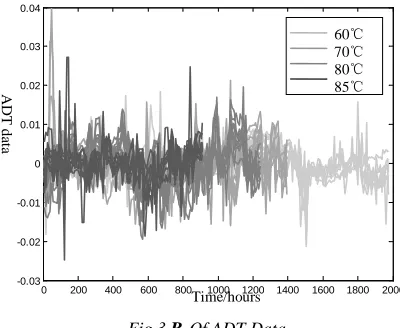
The Dt of each system is set as a linear form. The
model parameters are estimated utilizing all
performance parameters degradation data. Rt is
[image:5.612.315.517.146.308.2]shown in Fig.3.
Fig.3 Rt Of ADT Data
The prediction of Yt of each system at 60℃, 70
℃, 80℃and 85℃ by the multidimensional time
[image:5.612.91.291.329.493.2]series model is shown in Fig.4.
Fig.4 Multidimensional Prediction Of Yt
The prediction of the same ADT data is also processed based on the one-dimensional time series model respectively for comparison. This is shown in Fig.5.
Fig.5 One-Dimensional Prediction Of Yt
According to Fig. 4 and Fig. 5, it is obvious that compared with the prediction curves, the multidimensional time series prediction of the
amplitude Yt more closely models the original
performance than the one dimensional time series method.
Given the failure threshold of each performance parameter as 96% of the initial value, the failure time of each of the performance parameters are shown in Table II.
Table II Failure Time (Hours)
Temperature 60℃ 70℃ 80℃ 85℃
Sys. 1
Perf. 1 3080 >2112 1688 >1712
Perf. 2 >3416 2072 1688 1672
Perf. 3 2968 >2112 >1880 1672
Sys. 2
Perf. 1 >3416 1720 1488 1608
Perf. 2 3184 1792 1608 1328
Perf. 3 >3416 2040 1808 1632
Sys. 3
Perf. 1 3400 >2112 1736 >1712
Perf. 2 >3416 1704 1720 >1712
Perf. 3 >3416 1896 1648 1528
The reliability evaluation of each unit is the minimum failure time prediction across all performance parameters for each unit. The predicted failure time distribution is determined by the Pearson chi-square Goodness of Fit Test. Table III shows the results of the Pearson chi-square test.
Table III Pearson Chi-Square Test Of Failure Time Distribution
Temp. 60℃ 70℃ 80℃ 85℃ Ave.
Lognorm 0.158 1.362 1.362 0.158 0.960
Weibull 0.455 0.833 2.779 0.455 1.356
0 500 1000 1500 2000 2500 3000 3500
0.95 0.96 0.97 0.98 0.99 1 1.01 1.02 1.03 1.04
A
D
T da
ta
Time/hours
60℃
70℃
80℃
85℃
Prediction
0 500 1000 1500 2000 2500 3000 3500
0.95 0.96 0.97 0.98 0.99 1 1.01 1.02 1.03 1.04
A
D
T da
ta
Time/hours
60℃
70℃
80℃
85℃
Prediction
0 200 400 600 800 1000 1200 1400 1600 1800 2000
-0.03 -0.02 -0.01 0 0.01 0.02 0.03 0.04
A
D
T da
ta
Time/hours
60℃
70℃
80℃
85℃
0 200 400 600 800 1000 1200 1400 1600 1800 2000
0.96 0.97 0.98 0.99 1 1.01 1.02 1.03 1.04 1.05
A
D
T da
ta
Time/hours
60℃
70℃
80℃
[image:5.612.94.296.548.705.2]According to Table III, Lognormal distribution is the best fit for failure time distribution.
The reliability evaluation for test-stress levels is converted into the use-stress level by establishing relationship between median failure time and test-stress levels, which is established assuming an Arrhenius accelerated model. That is
[image:6.612.89.298.188.411.2]ln
µ
=
3454.04 /
S
−
2.4015
Fig.6 shows median failure time and temperature
stress level relationship based on a
multidimensional time series analysis.
Fig.6 Median Failure Time & Temperature Relationship Based On Multidimensional Time Series
Fig.7 shows median failure time and temperature stress level relationship based on a one-dimensional time series analysis for comparison.
Fig.7 Median Failure Time & Temperature Relationship Based On One-Dimensional Time Series
The error of the prediction is defined as the mean square error for all parameters of each system degradation measurement across all prediction points between the start point and last time point
before system failure. The predicted error is shown in Table IV.
Table IV Error Of Predictions
Model Multidimensional time series
Temp. 60℃ 70℃ 80℃ 85℃
Sys. 1 0.00114 0.00094 0.00142 0.00120
Sys. 2 0.00078 0.00111 0.00141 0.00116
Sys. 3 0.00132 0.00149 0.00091 0.00105
Model One-dimensional time series
Temp. 60℃ 70℃ 80℃ 85℃
Sys. 1 0.00231 0.00158 0.00234 0.00193
Sys. 2 0.00273 0.00143 0.00156 0.00251
Sys. 3 0.00156 0.00203 0.00148 0.00253
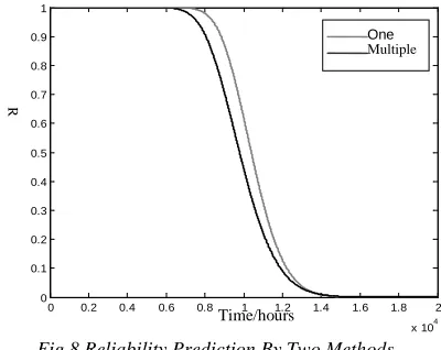
Fig.8 shows the reliability prediction at the
use-stress level 25℃, based on the multidimensional
[image:6.612.320.520.323.482.2]time series analysis and the one-dimensional time series analysis is shown for comparison.
[image:6.612.90.304.490.642.2]Fig.8 Reliability Prediction By Two Methods
Table V. shows failure time distribution parameters at the use-stress level based on the multidimensional time series analysis with the one-dimensional time series analysis for comparison.
Table V Failure Time Distribution Parameters
Model
Multidimensional time series
One-dimensional
time series Lognormal
mean
9.1893 9.2493
Lognormal variance
0.1525 0.1268
Median failure time
9791.8 hours 10397.3 hours
According to Fig.8 and Table V, it could be concluded that reliability evaluations by a multidimensional model are more conservative than one-dimensional model. And according to Table IV, it could be concluded that reliability evaluations by a multidimensional model are more accurate
0 0.2 0.4 0.6 0.8 1 1.2 1.4 1.6 1.8 2
x 104
0 0.1 0.2 0.3 0.4 0.5 0.6 0.7 0.8 0.9 1
R
Time/hours
One
Multiple
20 30 40 50 60 70 80 90
1000 2000 3000 4000 5000 6000 7000 8000 9000 10000 11000
T/℃
M
edi
um
F
ailu
re
ti
me
acceleration model prediction lifetime Arrhenius model Reliability
20 30 40 50 60 70 80 90
1000 2000 3000 4000 5000 6000 7000 8000 9000 10000
T/℃
Medium
failure time
than one-dimensional model. Hence, the former is more credible than the latter.
6. CONCLUSIONS
This paper proposes a reliability evaluation method utilizing a multiple performance parameter system ADT based on a multidimensional time series modeling procedure.
(1) Compared with one-dimensional time series
analysis, the multidimensional time series analysis takes into account the interaction of multiple performance parameters on the performance degradation process.
(2) Based on the practice, the failure of systems
with multiple performance parameters is assumed to obey a competing failure rule that enables a solution for the failure determination problem given multiple system performance failure measures.
(3) To obtain a reliability evaluation for systems
with multiple performance parameters at the use-stress level, this paper proposed a conversion method based on a reliability evaluation across multiple system performance measures at test-stress level based upon a test acceleration model.
(4) According to the ADT data verification process
compared to a one-dimensional time series analysis, the prediction based on a multidimensional time series analysis of the amplitude observed in ADT more closely model the original curve. Thus any failure time
or reliability prediction based on
multidimensional time series method was demonstrated to be more conservative, accurate and credible.
REFERENCES:
[1] Wang Li; Li Xiaoyang; Jiang Tongmin, “SLD
Constant-Stress ADT Data Analysis based on
Time Series Method”, 8th International
Conference on Reliability, Maintainability and Safety, 2009.
[2] Victor Chan, William Q. Meeker, “Time Series
Modeling of Degradation Due to Outdoor Weathering”, Communications in Statistics - Theory and Methods, 37:3,408-424 , 2008.
[3] Wang, J., Zhang, T., “Degradation prediction
method by use of autoregressive algorithm,”
IEEE Transactions n Industrial Technology, 21-24, Page(s):1-6, April 2008.
[4] Xu, L., “Study on Fault Prognostic and Health
Management for Electronic System”, Ph.D. Thesis, University of Electronic Science and Technology of China, 2009.
[5] Bachmann, S. M., “Using the Existing Spectral
Clutter Filter With the Nonuniformly Spaced Time Series Data in Weather Radar,” IEEE Geoscience and Remote Sensing Letters, Vol. 5, No. 3, July 2008.
[6] V. Serdobolskii, “Multivariate Statistical
Analysis”, Springer, 2000.
[7] Shuyuan He, “Applied Time Series Analysis”,
Peking University Press, 2003.
[8] Wang Li, Li Xiaoyang, Jiang Tongmin,
“CSADT Reliability evaluation based on DAD using Time Series Method ”, Proceedings of Annual Reliability and Maintainability Symposium (RAMS2011), 2011.
[9] Wang Li, Li Xiaoyang, Wan Bo, “Step-Stress