R E S E A R C H
Open Access
A Monte Carlo localization method based
on differential evolution optimization
applied into economic forecasting in
mobile wireless sensor networks
Miao Qin
1and Rongbo Zhu
2*Abstract
The localization of sensor node is an essential problem for many economic forecasting applications in wireless sensor networks. Considering that the mobile sensors change their locations frequently over time, Monte Carlo localization algorithm utilizes the moving characteristics of nodes and employs the probability distribution function (PDF) in the previous time slot to estimate the current location by using a weighted particle filter. However, it also has the problem of insufficient number of valid samples, which further affects the node’s localization accuracy. In this paper, differential evolution method is introduced into the Monte Carlo localization algorithm. The sample weight is taken as the objective function, and differential evolution algorithm is implemented in sample stage. Finally, the node position is estimated by making the sample close to the actual location of the node instead of being filtered out. The simulation results
demonstrate that the proposed algorithm provides a better position estimation with less localization error.
Keywords:Economic forecasting, Wireless sensor networks, Valid sample, Localization, Differential evolution
1 Introduction
In the era of big data, economic forecasting is crucial. The nodes’ localization in wireless sensor networks (WSNs) refers to the process of obtaining their own or monitoring the geographic position of the object in a certain way [1]. It is important to obtain the sensor node’s location, and the monitoring data will be mean-ingless without location information. For instance, in precision agriculture, the sensor nodes can gather data of light intensity, humidity, and temperature, which must be accompanied by the coordinates of the collec-tors [2]. Without such positional information, the obser-ver cannot match the data with the region and make an appropriate decision. Meanwhile, the exact location information of sensor nodes are of great help in improv-ing the efficiency of network routimprov-ing [3]. Since the wire-less sensor network consists of a large number of sensors and the topology often change especially for the
environment with mobile nodes, each sensor nodes need to be equipped with a positioning system, such as GPS. Due to the high cost of GPS, it is not suitable for low-power and low-cost requirements of sensor nodes [4]. In addition, for some special application scenarios (such as shopping malls), the positioning performance of GPS will be affected [5]. Generally, there are two types of nodes in wireless sensor networks, which are called as anchor node and blind node. Anchor nodes, which are usually configured manually or equipped with a GPS re-ceiver to obtain their location information, can obtain position coordinates by themselves. However, the pro-portion of anchor nodes in all sensor nodes is relatively small. Comparatively, blind node can only acquire its position information by using the localization algorithm.
The rest of the paper is structured as follows. The motivation for this work is discussed in Section 2. In Section 3, we derive Monte Carlo localization methods based on differential evolution optimization (MCL-DE) for valid samples in mobile wireless sensor networks. In Section 4, a comparative performance evaluation is
* Correspondence:[email protected]
2College of Computer Science, South-Central University for Nationalities,
Wuhan 430074, China
Full list of author information is available at the end of the article
carried out. Finally, concluding remarks and future work are given in Section5.
2 Related work
So far, the research of node’s localization algorithm in wireless sensor networks has been widely carried out. The main purpose of sensor localization is to deter-mine the location of sensors in WSNs via noisy mea-surements, and most of the methods for localization can be classified into geometrical techniques, multidi-mensional scaling, stochastic proximity embedding, convex and nonconvex optimization, and hybrid. In range-based measurement localization, the major task is to find the accurate position in non-line-of-sight (NLOS) paths. These range-based measurements may include time-of-arrival (TOA) [6], time-difference-of-arrival (TDOA) [7], angle-of-arrival (AOA) [8], and received signal strength (RSS). After evaluating the distance between the nodes, the position of the blind node can be obtained based on three edge-measuring or maximum likelihood methods [9].
Range-based localization requires additional hardware and power consumption, so nodes can achieve accurate positioning resolution. However, the demand to reduce hardware dependency and energy cost has been the focus of academia and industry, and some researchers also proposed a range-free localization algorithm [10]. Usually, range-free location algorithms demonstrate poor performance in the aspect of positioning accuracy than the range-based localization algorithm, but it does not need additional hardware support and can meet many requirements in the scenarios with rough localization effect. In [10], an indoor localization strategy for mini-UAV in the presence of obstacles is proposed, in which the signal propagation state is identified according to the prior probability and statistics of TDOA and RSS measurements. In [11], a NLOS identifi-cation and weaken algorithm with machine learning is proposed to identify and weaken the NLOS error by means of support vector machine (SVM), which can em-ploy a large number of data samples to train the SVM classifier. A voting matrix is constructed to weaken the error of non-line-of-sight and obtain the candidate pos-ition in accordance with the error characteristics of LOS measurements and NLOS measurements. Then, the re-sidual weighted method is used to obtain the final posi-tioning results. Base on the range distance in each sampling period, Cui et al. [12] use multidimensional scal-ing localization algorithm to evaluate the location of the target and fit the result of the estimation by polynomial. The estimation results of current position can be cor-rected effectively, and the method is proven to achieve high positioning accuracy in indoor environment.
In recent years, interacting multiple model (IMM) combined with filtering technology has become a hot re-search topic. Chen et al. [13] combine IMM and extended Kalman filtering to achieve accurate posi-tioning in NLOS environment. Zhang et al. [14] propose a Kalman filter model based on interacted multiple objectives to filter the measured distance under the LOS/NLOS mixed environment, in which the IMM algorithm is applied to filter the distance, and then the extended Kalman filtering algorithm is used to realize the positioning. Under the IMM framework, Ru et al. [15] employ hidden Markov ran-dom field to solve the nonlinear Bayesian estimation problem and improve the positioning accuracy. Nevertheless, the above methods are put forward in the premise of accurate NLOS error parameters. But in the actual environment, the parameters of NLOS error are usually unknown. In [16], an Advanced DV-Hop localization algorithm is proposed to reduce the localization error without requiring additional hardware and computational costs. The hop-size of the anchor node is obtained base on the distance measurement of unknown nodes, and the weighted least square algorithm is introduced to decrease the inherent error in the estimated distance between the anchor and an un-known node. In [17], a mixed localization algorithm for wireless sensor networks based on APIT is pro-posed to deal with the problem of low localization ac-curacy with dense distribution of beacon nodes and low coverage ratio in the sparse case.
3 System and network model 3.1 Monte Carlo localization method
Monte Carlo localization method was originally applied to the field of robot localization, and the distinction be-tween the robot localization and the sensor node’s positioning in mobile wireless sensor network is very remarkable [18]. In the process of robot walking, the robot’s CPU is equipped with a map, and the path guidance will be abided to the prescribed route in the map. However, all sensor nodes will move in a ran-dom mode in the designated area. The location method based on Monte Carlo is actually a continu-ous iterative Bayesian filter, and the basic idea is to make use of some weighted samples to represent the posterior probability density distribution of the esti-mated state, so as to obtain the solution of the node position. This method can be applied to non-Gauss, nonlinear and multidimensional system, which is beneficial for the characteristics including flexibility, easy to implement, and suitable for parallel process-ing. Those merits make it very suitable for node localization in wireless sensor networks.
Since that the neighbor nodes within the range of transmission radius can communicate with each other, the known information from anchor nodes can be used to assist blind node’s localization [19]. The Monte Carlo localization method is based on the Bayes filtering the-ory, and the main idea is by utilizing the new observa-tion from the adjacent anchor nodes within the range, the sample and filter steps will be repeated until enough valid samples can be obtained. Then, the blind node can estimate its current location as it completes the move-ment [20]. Therefore, the resolution of the blind node’s localization can be transferred into the posterior prob-ability density function. Lettbe a discrete time series,xt is the state of hidden Markov processes with initial dis-tributionP(x0),xt∈Rnx wherenxis the dimension of state vector. Transfering equation P(xt|xt-1) demonstrates the dynamic features of the state space model. Meanwhile, the observation sequences {o1, o2, o3, …, ot} are inde-pendent of each other at a given node’s position {x1, x2,
x3…, xt}, whereOt∈Rn0 and n0 is the dimension of the observation vector.P(ot|xt) is the observation equations, and it denotes the probability of observed values under the condition of a given positionxt.
Suppose that the location of mobile nodes satisfies Markov assumptions in mobile wireless sensor net-works, and the observation and node’s position are independent. This indicates that the observations only depend on the current position, and the current pos-ition xt lies on the position xt-1 at the previous time interval. Thus, the resolution of the location of blind nodes can be converted into a posteriori probability density function p(xt|o0t).
The posterior probability density function at time t
can be approximated by some weighted samplesðxit;witÞ,
where δ is the Dirac-delta function, and N represents
the number of samples for the node’s location. xi
t is a
possible sample of node at timet, and wi
t is a
nonnega-tive weight.
The sample weight will be updated as the following formula:
whereϕis the adjustment function being relevant to xi
t; xi
0:i−1;o0:t.
Since the sensor nodes move randomly in a certain area, and the size and direction of motion are unknown. The maximum speed of motion is limited to v0; the current position of the node must be in the circle area with the center point of the position at the previous mo-ment and a radius of maximum moving speed v0. Then, the sample probability distribution at the present mo-ment can be expressed as:
p zð tjzt−1Þ ¼
where d(zt,zt-1) denotes the Euclidean distance between
the sample at current and previous time.
3.2 Objective function optimization based on sample weight
The anchor nodes will broadcast the ID identification and location information periodically. Suppose that the broadcast message from the set of anchor nodes within one-hop S(s) and the two-hop T(s) can be received by the blind node at the current time, the samples that does not satisfy the condition can be rejected in the process of filtering prediction with reference to the observation requirement. The eligible samples must be within the communication radius of a neighbor anchor node; meanwhile, the distance between the sample and the two-hop anchor node must be less than two times of the communication radius. Thus, the constraints can be expressed as:∀s∈S(s),d(z,s)≤r∩∀s∈T(s),r<d(z,s)≤2r.
According to the N samples of the position and the value of ðzi
t;witÞ, the current position of the blind node
CurPOSt¼
XN
i¼1
zitwit ð4Þ
The sample weights, i.e., the proportion of the samples in the final positioning result, are a measure of the merits of the standard sample. The observation results
Otof ordinary nodes are composed of a one-hop neigh-bor anchor node set S, two-hop anchor node set Tand the set of normal nodes within the transmission range
TR, andOt=S∪T∪TR. Considering the size of the sam-ple constraint box, the confidence function is introduced into the localization results to reflect the confidence de-gree of nodei at time t, of which the value depends on the size of the constraints from sampling box.
wit¼p Otjz
length of the entire region.
ifs∈S,
where the sample weight is regarded as the objective function of the optimization.
3.3 The process of sampling optimization
Owing to the similarity of the idea between the differen-tial evolution algorithm and the Monte Carlo algorithm, the individual vector in differential evolution algorithm can be regarded as a particle sample. Moreover, if the population number is equal to the size of the particle set, then the population in the differential evolution al-gorithm is equivalent to the particle set in the Monte Carlo localization algorithm. Hence, it is convenient to involve differential evolution method into Monte Carlo localization algorithm. In the sampling phase, the sample weight is taken as the objective function, and the differ-ential evolution algorithm is implemented. Then, the ac-tual position of sample can be approached to the node to be positioned actively rather than to be filtered, and the final estimate of node’s position can be obtained. The detailed steps are as follows:
1. Initialization: According to the initial variable interval [zmin,zmax] of the variable given by the
specific problem, the linear transformation can be given as:
zijð Þ ¼0 zminþ randð0;1Þ ðzmax−zminÞ ð8Þ
where zij(0) denotes the j-th variable of individual i;
rand(0,1) represents the random number with the range of [0,1].
2. Mutation: The different individualsZr1(g),Zr2(g),
andZr3(g) are selected, and the perturbation vectors
are generated according to the following method:
viðgþ1Þ ¼zr1ð Þ þg ηðzr2ð Þg −zr3ð Þg Þ ð9Þ
where η is the control factor to adjust the amplitude of the individual difference, and Zi(g) denotes the i-th
indi-vidual in populationg.
During the process of evolution, it is necessary to determine whether the variables satisfy the boundary conditions to ensure the validity of the solution. Otherwise, the variable will be generated randomly repeatedly.
3. Cross operation: The crossover between individuals {Zi(g)} of the g-th generation and its mutant
whereρis the crossover probability.
4. Select operation: Greedy algorithm is applied to select the individuals with high fitness to enter the next generation:
ziðgþ1Þ ¼ uiðgþ1Þ; f uð iðgþ1ÞÞ≤f zð ið Þg Þ zið Þg ; else
ð11Þ
3.4 Self-adaption of scaling factor and cross probability
Since the selection of ηand ρ is the key to the behavior and performance of differential evolution and affects the convergence of the algorithm directly,ηandρshould be varied with fitness and evolutionary algebra dynamically.
well as to ensure the convergence of difference. Based on the above analysis, η can be adjusted adaptively ac-cording to the following formula:
η¼ ln
where f indicates the fitness value of individuals to be
mutated, favg is the average fitness value of the
popula-tion, andfbestis the maximum fitness value in the
popu-lation. At the beginning of the algorithm, the difference
betweenfavg and fbestare very large, and there is almost
no possibility of local convergence. With the progress of
the generation evolution, the gap between favg and fbest
will decrease. Meanwhile,fmerges a decrease trend and
the speed for converging to the optimum solution will continue to be accelerated gradually, which reduce the risk of falling into local convergence.
The probability of crossover demonstrates the possibil-ity that the genes for mutating individuals can be se-lected to a new individual. Hence, the adaptive function is presented to adjust the value ofρdynamically accord-ing to the senior generation individual. Initially, ρ is set as a relatively small valueρ0, which ensures the popula-tion diversity with a low probability of crossover. With the evolution of the individual, the individuals begin to converge gradually. At this time, the increase ofρ value will not only improve the variation of gene selection’s probability but also speed up the convergence rate. When the ρ=ρ*, the value of ρ will increase no longer and remain stable. The value ofρcan be given as:
ρ¼
whereGindicates the generation.
The value of sample weights is equal to 0 or 1, and value 1 denotes that the corresponding sample can sat-isfy with the filtering condition. When the number of sample weights reaches to N or the maximum gener-ation G, the evolutionary algorithm terminates. Finally, the estimation of node’s localization can be obtained by using the sampled nodes being selected optimally from the differential evolution algorithm.
3.5 Obtain the positioning results
Before employing the final N samples to calculate the localization results, the weights of the samples should be normalized as:
Then, the estimation of the coordinate of the nodeiat timetcan be obtained by theNsamples:
xti ¼X
Considering that the actual position of the nodes be included in the constraint sampling box, the range of (xmin,xmax;ymin,ymax) denotes that all the samples are ob-tained in the sample box. The sample within the range must satisfy the constraints of the weighted average. Therefore, the actual node’s localization error must be less than the maximum difference between the estima-tion of node’s position and the boundary coordinates of sampling box. We have:
In this section, we will conduct the experiments to com-pare our algorithm with the traditional method, for ex-ample, RMCL [18] and DLS [19] in terms of the localization precision, sample size, maximum velocity, and the density of anchor nodes. In order to verify the indicators objectively, the parameters of the experiments are set to be identical in different scenarios. The specific parameters are set in details as follows: the number of sensor nodes is 320, the deployment area is 500 × 500 m2; the transmission radius of sensor node is r= 50 m; the number of valid samples is N= 50. The mo-tion process of the node employs RWP model [20], and the maximum moving speed vmax= 0.2r. Besides, the main parameters of differential evolution are set as:
η=0.8,ρ0= 0.4, andρ* = 0.9.
To evaluate the effects on the localization algorithm by setting different parameters, the average localization error and the number of candidate samples are regarded as key indicators. Among them, the number of candidate samples reflects the number of times as the sampling process is executed for obtaining the valid samples. Usu-ally, the lesser the number of candidate samples is, the higher the success rate of sampling can obtain.
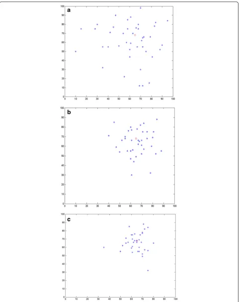
Figure1shows the localization performance of the sam-ples of different generations with differential evolution.
algorithm will be executed, which uses the sample weight as objective function. Since the observation re-sults from the normal nodes only involve anchor nodes, the sample weight is equal to 0 or 1. Next, the derived sample weight is equal to 1 and it can be remained in the next generation. Otherwise, the parents’sample can only reserve in the next generation. After several genera-tions being produced, plenty of samples can be satisfied with the filtering conditions, most of which is close to the actual position of the node. As can be seen from Fig.1, compared with the initial samples, the samples of subsequent generation with differential evolution are closer to the actual location of the node.
Figure2 shows the comparison of convergence of the algorithm. As can be seen from the result, the localization accuracy of all algorithms demonstrates ab-solutely low-quality in the initial stage. With the time goes, the number of valid samples is getting more and more, and the accuracy is corrected by iteration. There-fore, the localization error decreases and fluctuates in a relatively stable range. During the whole convergence phase, we can observe that the average error in MCL-DE shows approximately 21.23% lower than RMCL, about 35.42% lower than DLS. Generally, the speed and direction of the node are unknown except for the maximum velocity. The maximum velocity and previous position can be utilized to predict the constrained sampling area in current time.
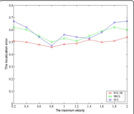
When the maximum moving speed is slow, the size of the sampling box based on the moving velocity is rela-tive small. Apparently, the actual position of the nodes will be of high probability to fall outside of the sampling box and the localization results will be very poor. With the increase of the maximum velocity, the node will be able to establish a better sampling box, which can con-tain the actual position with high probability, to reduce
the localization error. However, excessive value of the maximum velocity of node can constraint the size of sampling box and result in the increase of the average node’s localization error and it can be seen from Fig. 3. In the process of the whole trend, the MCL-DE algo-rithm always keeps the advantage over other methods in localization accuracy.
The number of the candidate samples depends on the size of sampling box, and Fig. 4 demonstrates the rela-tionship between the maximal moving velocity and the number of candidate samples. For DLS, since the effect of sampling is entirely determined by the maximum vel-ocity of the node, the increase of the maximum velvel-ocity of movement will extend the range of the sample box as well as increase the number of final candidate samples. However, the sampling constraint box of MCL-DE is mainly composed of one-hop and two-hop neighbor an-chor nodes, and the size of the sample box will be pri-marily restricted by the anchor nodes. That is, when the maximum velocity of motion is increased, the number of candidate samples will not change obviously due to the stable observation results from the anchor nodes.
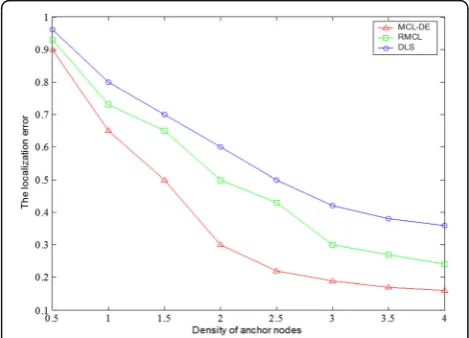
Next, the experiment is conducted to verify the effect on localization error in different density of anchor nodes. As can be seen from the Fig.5, the samples being selected optimally can approximate to the actual pos-ition, and the results with weighted average calculation make the average localization error as small as possible. From the results, the trend of average localization error in all algorithms shows very clearly. Comparatively, the average location error in different densities of anchor nodes in MCL-DE is less than RMCL and DLS. Espe-cially, when the density of anchor nodes is set to 1, the average localization error of MCL-DE can be less than RMCL about 16.59% and DLS about 33.43%.
Moreover, the increase of the anchor node’s density will bring about more constraint conditions for filtering process. As a result, the filtration rate of samples will in-crease. As shown in Fig. 6, with the increase of anchor node’s density, the number of candidate samples in RMCL and RMCL grows remarkably. In contrast, the growth of DLS algorithm is greater because it does not make use of the anchor node’s information at the sam-pling stage. Due to fixed samples for initial operation, the number of candidate samples remains constantly.
5 Conclusions
After obtaining a certain number of initial samples, we select the weight of the sample as the objective function of the optimization and present the differential evolution algorithm to obtain valid samples rather than perform initial sample filtering and resampling. Finally, the node position is estimated by making the sample close to the
actual location of the node instead of being filtered out. The simulation result demonstrates that the proposed algorithm provides a better position estimation with less localization error. In the future, we will study and valid-ate the signal strength indicator to improve the perform-ance of our method in aspect of computational and communication costs. And we are also planning to dis-cuss the challenges and open research issues related to the parameters and focus on the localization accuracy of range-free schemes.
Acknowledgements
This work is supported by the National Natural Science Foundation of China under grants 61772562 and 61272497, the Youth Elite Project of State Ethnic Affairs Commission of China, and the Hubei Provincial Natural Science Foundation of China for Distinguished Young Scholar under grant 2017CFA043.
Authors’contributions
QM and RBZ contributed to the conception and algorithm design of the study. RBZ contributed to the acquisition of the simulation. QM contributed to the analysis of simulation data and approved the final manuscript. Both authors read and approved the final manuscript.
Authors’information
Qin Miao is an undergraduate student at the School of management in Wuhan University of Technology. His research interests lie in wireless sensor networks, information management, and economic forecast.
Rongbo Zhu received the B.S. and M.S. degrees in Electronic and Information Engineering from Wuhan University of Technology, China, in 2000 and 2003, respectively, and the Ph.D. degree in communication and information systems from Shanghai Jiao Tong University, China, in 2006. From August 2011 to August 2012, he was a research scholar in the Bradley Department of Electrical and Computer Engineering, Virginia Tech, USA. His research interests include mobile computing, protocol design, and performance optimization in wireless networks. He has published over 70 papers in international journals and conferences in the areas of mobile computing and wireless communications and networks. He received the Outstanding B.S. Thesis and M.S. Thesis awards from Wuhan University of Technology in 2000 and 2003, respectively. Dr. Zhu serves as an Editorial Board member of 6 international journals and the Lead Guest Editor for 5 international journals. He has been actively involved in around 30 international conferences.
Competing interests
The authors declare that they have no competing interests.
Fig. 4The number of optimal samples with maximum velocity
Fig. 5Localization error with anchor nodes
Publisher’s Note
Springer Nature remains neutral with regard to jurisdictional claims in published maps and institutional affiliations.
Author details
1School of management, Wuhan University of Technology, Wuhan 430070,
China.2College of Computer Science, South-Central University for
Nationalities, Wuhan 430074, China.
Received: 5 January 2018 Accepted: 20 January 2018
References
1. R Stoleru, T He, SS Mathiharan, SM George, JA Stan-kovic, Asymmetric event-driven node localization in wireless sensor networks. IEEE Trans. Parallel Distrib. Syst.23(4), 634–642 (2012)
2. A Kumar, A Khosla, JS Saini, SS Sidhu, Range-free 3D node localization in anisotropic wireless sensor networks. Appl. Soft Comput.34(2), 438–448 (2015) 3. F Shahzad, TR Sheltami, EM Shakshuki, Effect of network topology on
localization algorithm’s performance. J. Ambient Intell. Humanized Comput. 7(3), 445–454 (2016)
4. N Iliev, I Paprotny, Review and comparison of spatial localization methods for low-power wireless sensor networks. IEEE Sensor15(10), 5971–5987 (2015) 5. SP Singh, S Sharma, Range free localization techniques in wireless sensor
networks: a review. Procedia Comput. Sci.57(2), 7–16 (2015) 6. I. GCuvenc¸ and C. C. Chong, A survey on TOA based wireless
localization and NLOS mitigation techniques, IEEE Commun. Surveys Tuts., 11(3): 107–124, 2009.
7. KC Ho, XN Lu, L Kovavisaruch, Source localization using TDOA and FDOA measurements in the presence of receiver location errors: analysis and solution. IEEE Trans. Signal Process.55(2), 684–696 (2007)
8. YS Lee, JW Park, L Barolli, A localization algorithm based on AOA for ad-hoc sensor networks. Mobile Inf. Syst.8(1), 61–72 (2012)
9. J Teng, H Snoussi, C Richard, R Zhou, Distributed variational filtering for simultaneous sensor localization and target tracking in wireless sensor networks. IEEE Trans. Veh. Technol.61(5), 2305–2318 (2012)
10. I Sharp, K Yu, T Sathyan, Positional accuracy measurement and error modeling for mobile tracking. IEEE Trans. Mobile Comput.11(6), 1021–1032 (2012) 11. Z Xiao, H Wen, A Markham, et al., Non-line-of-sight identification and
mitigation using received signal strength. IEEE Trans. Wirel. Commun.14(3), 1689–1702 (2015)
12. W Cui, CD Wu, W Meng, et al., Dynamic multidimensional scaling algorithm for 3-D mobile localization. IEEE Trans. Instrum. Meas.65(12), 2853–2865 (2016) 13. BS Chen, CY Yang, KF Liao, Mobile location estimator in a rough wireless environment using extended Kalman-based IMM and data fusion. IEEE Trans. Veh. Technol.58(3), 1157–1169 (2009)
14. JY Ru, CD Wu, ZX Jia, et al., An indoor mobile location estimator in mixed line of sight/non-line of sight environments using replacement modified hidden Markov models and an interacting multiple model. Sensors15(6), 14298–14327 (2015)
15. K Shrawan, DK Lobiyal, An advanced DV-hop localization algorithm for wireless sensor networks. Wireless Pers Commun.71(2), 1365–1385 (2013) 16. B-N Vo, S Singh, A Doucet, Sequential Monte Carlo methods for multi target
filtering with random finite sets. IEEE Trans. Aerosp. Electron. Syst.41(4), 1224–1245 (2005)
17. Pezzilli R, Venturi M, Morselli-Labate A M, et al, Differential evolution algorithms solving a multi-objective, source and stage location-allocation problem. Ind. Eng. Manag. Syst.14(1),11–21, (2015)
18. Y Wang, Z Cai, Y Zhou, et al., An adaptive tradeoff model for constrained evolutionary optimization. IEEE Trans. Evol. Comput.12(1), 80–92 (2008) 19. J-P Sheu, W-K Hu, J-C Lin, Distributed localization scheme for mobile sensor
networks. IEEE Trans. Mob. Comput.9(4), 516–526 (2010)