Multiple importance sampling revisited: breaking the bounds

R E S E A R C H

Open Access

Multiple importance sampling revisited:

breaking the bounds

Mateu Sbert

, Vlastimil Havran

and Laszlo Szirmay-Kalos

Abstract

We revisit the multiple importance sampling (MIS) estimator and investigate the bound on the efficiency

improvement over balance heuristic estimator with equal count of samples established in Veach’s thesis. We revise the proof for this and come to the conclusion that there is no such bound and henceforth it makes sense to look for new estimators that improve on balance heuristic estimator with equal count of samples. Next, we examine a recently introduced non-balance heuristic MIS estimator that is provably better than balance heuristic with equal count of samples, and we improve it both in variance and efficiency. We then obtain an equally provably better one-sample balance heuristic estimator, and finally, we introduce a heuristic for the count of samples that can be used when the individual techniques are biased. All in all, we present three new sampling strategies to improve on both variance and efficiency on the balance heuristic using non-equal count of samples.

Our scheme requires the previous knowledge of several quantities, but those can be obtained in an adaptive way. The results also show that by a careful examination of the variance and properties of the estimators, even better

estimators could be discovered in the future. We present examples that support our theoretical findings.

Keywords: Global illumination, Rendering equation analysis, Multiple importance sampling, Monte Carlo

AMS Subject Classification: primary Computer Graphics G.3 Mathematics of Computing/PROBABILITY AND STATISTICS probabilistic algorithms; Computer Graphics G.3 Mathematics of Computing / PROBABILITY AND STATISTICS probabilistic algorithms; secondary Computer Graphics G.3 Mathematics of Computing / PROBABILITY AND STATISTICS probabilistic algorithms

1 Introduction

Themultiple importance sampling(MIS) estimator [1,2], and in particularbalance heuristic, which is equivalent to the Monte Carlo estimator with a mixture of probabil-ity densprobabil-ity functions (pdfs), has been used for many years with a big success, being a reliable and robust estimator that allows an easy and straightforward combination of different sampling techniques. MIS with balance heuris-tic estimator has been almost exclusively used with equal count of samples for each technique, mainly following the recommendations based on certain quasi-optimality the-orems in Veach’s thesis. Specifically, these thethe-orems stated that a balance heuristic estimator could not be worse

*Correspondence:[email protected]

1_{School of Computer Science and Technology, Tianjin University, Tianjin, China} 2_{Department of Informatics, Applied Mathematics and Statistics, University of}

Girona, Campus de Montilivi, Girona, Spain

Full list of author information is available at the end of the article

thanntimes any other MIS estimator with equal count of samples where n is the number of combined meth-ods. In papers addressing the variance of MIS, strategies were assumed to have equal number of samples [3, 4], and the combination of MIS with jittered sampling was studied in [5].

MIS is often used in rendering applications of computer graphics [6] where the reflected illumination is the prod-uct of the intensity in the illumination direction that can be represented by an environment map, and the proba-bility of the reflection from a surface. As it is not feasible to sample with this product of two functions, sampling mimics either directions from where reflection is likely or directions of high intensity. The first approach is called light source sampling and the second approach is called BRDF sampling after the name of the bidirectional reflec-tion distribureflec-tion funcreflec-tion (BRDF).

Lu et al. [7] propose an improvement to balance heuris-tic estimators for environment map illumination by using a Taylor’s second order approximation of the variance around the equal weights 1/2 to obtain the counts of samples according to the BRDF and the environment map, which is accurate only if the optimal sample num-bers are not too far from equal sampling. Heuristics have also been used that prefer certain sampling meth-ods based on the local properties, for example, BRDF sampling is advantageous on highly specular surfaces and light source sampling on diffuse surfaces. Pajot et al. pro-posed a framework, called representativity, to develop such heuristic [8]. Havran and Sbert [9, 10] introduce a heuristic for unbiased techniques based on assigning a count of samples proportional to the inverse of the variance of each technique that in some cases seemed to put into question the quasi-optimality rules of equal sampling. More recently, based on the analysis of the vari-ance of MIS estimators, Sbert et al. [11] discovered a MIS non-balance heuristic estimator that is provably bet-ter than balance heuristic with equal count of samples. The introduction of costs into those schemes allowed an even bigger increase in efficiency. We improve on their work by clarifying the quasi-optimality rules in Veach’s thesis by introducing new balance heuristic estimators that are provably better than balance heuristic with equal count of samples, and by introducing a new heuristic valid when the individual estimators are biased. We believe that our work can inspire new provably better estima-tors or at least sound heuristics for heuristically better estimators.

Putting our results in a wider perspective, we should consider adaptive variance reduction methods that learn some properties of the integrand, e.g., the location of its peak, and refine the sampling strategy on-the-fly by analyzing the samples that have been already generated. In case of mixing different pdfs with which sampling is straightforward, the weights of the individual meth-ods are the target of the adaptation. Adaptive methmeth-ods can be imagined as a sequence of Monte Carlo quadra-ture steps and parameter estimation steps. Care should be exercised to implement adaptive methods since mak-ing the samplmak-ing pdf dependent on the generated samples might make the estimator biased, which can be attacked by freezing the adaptation after certain samples letting the approach be consistent. Another challenge is the control of the adaptation with randomly sampled, i.e., noisy data. To handle this, adaptive MCMC approaches often choose an artificial but robust criterion, like the acceptance rate, instead of the variance of the estimation [12,13]. In com-puter graphics, this technique has been used to control the mutation of MCMC methods [14, 15] and to dis-tribute different numbers of samples among the different techniques [16].

Owen and Zhou [17] survey the principles of adaptively mixing different sampling strategies, including defensive importance sampling and the simultaneous application of control variates and importance sampling. They also investigate MIS and point out that there is a room for improvement. Douc et al. [18] investigated the population Monte Carlo method and derived sufficient convergence conditions for adaptive mixtures, and also iterative for-mulae for the optimal weights [19]. As population Monte Carlo explores the sampling space with a Markov stochas-tic process, it uses the information of only the current samples directly. Cornuet et al. [20] improve this in their adaptive multiple importance sampling algorithm and present optimal exploitation of previous samples, which automatically stabilizes the process. Marin et al. [21] argue that the Markov property is important to be able to prove the consistency of the estimator, and the stability of the process can be achieved by increasing the sample size in each iteration.

In their recent work, Martino, Elvira et al. proposed adaptive population importance sampling [22] and gra-dient adaptive population importance sampling [23] that adapt the mean and the covariance of proposal Gaussian pdfs, and reported significant improvements with respect to MIS that keeps the individual proposal pdfs fixed. We note that in computer graphics the not continuous integrands may pose problems to such gradient-based methods. Elvira et al. also examined a discrete weight-ing scheme [24] where only a subset of available sampling strategies is selected with the aim of reducing the compu-tational complexity of the sampling process.

The rest of the paper is organized as follows: In Section2, we review the basic formulae for the variance of MIS. In Section3, we discuss Theorem 9.5 of Veach’s thesis and present a new proof for a slightly modified theorem. In Section4, we present a multi-sample balance heuristic estimator that is provably better than multi-sample balance heuristic with equal count of multi-samples. In Section 5, we obtain a provably better one-sample bal-ance heuristic estimator, and in Section6, we justify a new heuristic for the count of samples that does not require the individual techniques be unbiased. In Section 7, we discuss the results, and in Section8, summarize our con-clusions. Some proofs are given in AppendicesAandB, and numeric 1D examples are presented in AppendixC.

2 MIS variance analysis

We review here the variance of MIS estimators. The naming convention for the estimators is given in Table1.

2.1 General multi-sample MIS estimator

Table 1Naming convention for the MIS estimators in this paper. We will drop the superindex 1 from primary estimators when not strictly necessary

F Generic multi-sample MIS estimator

F Generic one-sample MIS estimator

F1 _{Generic one-sample MIS primary estimator}

ˆ

F Generic multi-sample MIS balance heuristic

estimator ˆ

F Generic one-sample MIS balance heuristic

estimator

In this combination scheme, sampling method i uses probability density functionpi(x)to generateNinumber of random samples {Xij}, (j = 1,. . .,Ni). If we have n

techniques, the total number of samples isn_i=1Ni =N. Integral estimatorFis unbiased, as its expected valueμis equal to integralI:

μ=E[F]=

The variance of the estimator is given in the proof of Theorem 9.2 of Veach’s thesis [2]. DefineFijas

Fij=wi(Xij)

f(Xij)

pi(Xij)

. (5)

For a fixed methodiand alljvalues, the estimators{Fij}

are independent identically distributed random variables with expected valueμi:

μi = E[Fij]=

and that the variance ofFijis

σ2

If samples are statistically independent, the variance of the integral estimator is

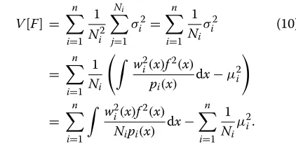
V[F] =

There are two different components of a MIS estima-tor that determine the variance of the estimates: weighting scheme wi and the number of samples Ni allocated to different methods. Weighting functions may or may not depend on the number of samples. Additionally, the num-ber of samples can be pre-determined, called the multi-sample model, or selected also randomly, which leads to theone-sample model.

2.2 Balance heuristic estimator

Veach defined a balance heuristic estimator setting the weights as the following:

wi(x)=

Nipi(x)

_n

k=1Nkpk(x)

. (11)

These weights lead to the following estimator:

ˆ

V[Fˆ]=

2.2.1 Balance heuristic with equal count of samples Observe that if we take equal count of samples for each technique, i.e., for alli,Ni = N/norαi = 1/n, then the

and the variance is equal to

V[Fˆeq]=

2.3 A provably better non-balance heuristic estimator Sbert et al. [11] introduced an estimator provably better than balance heuristic with equal count of samples. Taking the weights as in Eq.14, the estimatorFin Eq.1is

The estimatorsFijin Eq.5become

Fij= The variance, Eq.10, is then

V[F] = that we improve on balance heuristic with equal sampling by using estimator Eq. 19, up to the statistical error in estimating theσi,eqvalues.

Taking into account the costci of sampling with tech-nique i, the sample numbers that guarantee that we improve the efficiency (i.e., the inverse of cost times vari-ance) over balance heuristic with equal sampling are

Ni∝ σ√i,eq

ci

. (22)

3 Breaking the bounds for the relative acceleration

In this section, we investigate the bounds for the improve-ment on the variance of balance heuristic estimator with equal count of samples.

This problem has been attacked by Veach establishing an inequality (Theorem 9.5 of his thesis [2]) for the vari-ance of the balvari-ance heuristic estimator with equal count of samplingFˆeq:

V[Fˆeq]≤nV[F]+

n−1

N μ

2_{, (23)}

where F is any multiple importance sampling estima-tor using the same total number of samples N. Veach interpreted Theorem 9.5 as a proof of quasi-optimality of balance heuristic with equal count of samples, saying “According to this result, changing the Ni can improve the variance by at most a factor ofn, plus a small addi-tive term. In contrast, a poor choice of thewican increase variance by an arbitrary amount. Thus, the sample alloca-tion is not as important as choosing a good combinaalloca-tion strategy.”

The proof of Eq.23is based on the following inequal-ity, which compares a general multiple importance sample estimatorF with arbitrary number of samples{Ni} with the same estimator (i.e., using the same weights wi) but with equal count of samples,Feqas follows:

V[F]≥ 1

But this inequality is not valid when the weightswi(x) depend on the number of samplesNi, see AppendixAfor a proof. Just to give a single counter example, let us con-sider the case when zero variance estimator is possible by properly setting the number of samples, makingV[F] zero, but the equal count of samples estimator will not have zero variance. However, we show that Theorem 9.5 can be generalized to such cases as well, but it requires the full reconsideration of the original proof.

The interpretation by Veach of Theorem 9.5 is based on the assumption that additive termμ2(n−1)/N is small if the total number of samples,N, gets larger. However, denominatorN is implicitly included in the other terms of Eq.23 as well, thus the considered additive term is, in fact, not negligible. As a result, the selection of Ni sample numbers or weightsαican make a significant dif-ference in the variance, which is worth examining and opens possibilities to find better estimators.

3.1 One-sample balance heuristic

The general MIS one-sample primary estimator is

F1₌ wi(x)f(x) αipi(x)

, (25)

where techniqueiis selected with probabilityαi. It can be easily shown that it is unbiased, i.e., its expected value is μ. Using the balance heuristic weights,

wi(x)= αi

pi(x)

n

k=1αkpk(x)

, (26)

the estimator becomes theone-sample balance heuristic estimator,

ˆ

F1₌ f(x) kαkpk(x)

. (27)

One-sample balance heuristic is the same as the Monte Carlo estimator using the mixture of probabilities

p(x) = n_k=1αkpk(x),

n

k=1αk = 1. Theαivalues are called the mixture coefficients and represent the aver-age count of samples from each technique. The variance of this estimator can be obtained by the application of the definition of variance,

is the variance of the one-sample balance heuristic estimator with equal weights, and V

ˆ

F1_{the variance of the one-sample balance}

heuris-tic estimator with any distribution of weights{αk}, then the following inequality holds:

ProofThe variance of the one-sample balance heuristic with equal weights is

VFˆ_eq1= Observing that αmax ≤ 1, the following corollary is immediate.

Corollary 1

VFˆ_eq1≤nVFˆ1+(n−1)μ2. (32)

Equations29and32do not imply that the improvement with respect to the equal count of samples is limited by a factor ofn, sinceμcan be large in comparison with the variances. So, it is worth trying to obtainαivalues that can reduce the variance.

Equations29and32can be extended to the one-sample MIS in general using Theorem 9.4 of Veach’s thesis, which states that the variance of the one-sample MIS estimator is minimal when it is a balance heuristic one, i.e.,V[Fˆ]≤

V[F]. For instance, for Eq.32

VFˆ_eq1≤nVF1+(n−1)μ2. (33)

And forNsamples,

V

Observe that Eq.34is similar to Eq.23except for the fact that it holds for the one-sample estimator. UsingV[Fˆ]≤

V[Fˆ] (as shown in [11]) we also have:

4 A provably better balance-heuristic multi-sample estimator

In Section1, we reviewed two strategies for the allocation of samples to individual methods, balance heuristic with equal count of samples (Section 2.2.1) and non-balance heuristic with sample numbers proportional to the vari-ance (Section2.3). The variance of the latter is better than that of the equal count estimator. This section shows that we can do it even better if the sample allocation strategy of Section2.3is applied to balance heuristic.

We can use Theorem 9.2 from Veach’s thesis, which states that for any MIS estimatorF, the balance heuris-tic estimatorFˆ with the same count of samples asFhas always less variance up to an asymptotically decreasing factor, i.e.,

to obtain a provably better estimator than the one described in Section2.3. Let us now take the estimatorF

as Eq.19from Section2.3whereNi∝σi,eq. This is prov-ably better than the balance heuristic with equal count of samples,Fˆeq, i.e.,V[F]≤V[Fˆeq]. Thus,

Observe thatFˆis the balance heuristic estimator defined in Eq. 12 where theNi ∝ σi,eq. Similar results can be obtained for the case when the sampling cost is also taken into account, i.e. consider now asFthe MIS estimator with

Ni∝σi,eq/√ci.

Estimator Fˆ is now the balance heuristic estimator defined in Eq.12withNi ∝σi,eq/√ci.

The efficiency in this case is

_n

Thus, the relative difference between variances will be constant disregardingN. This is a similar situation to that encountered in Section3.

5 A provably better one-sample balance heuristic estimator

The variance of the estimator in Eq. 25 is the second moment minus the square ofμ:

V[F1]=

where the second momentsM2_i are defined as

M2_i = means minimizing the first term of the last equality in Eq.41. When the weights{wi(x)}are independent of the coefficients{αi}, we get the following theorem:

Theorem 2 When the weights{wi(x)}are independent of

the{αi}, the minimum variance in Eq.41is obtained when

αi∝Mi. (43)

variance is then given by substituting the optimal {αi} from Eq.43to Eq.41, resulting in

Vmin

F1 ₌

_n

i=1

Mi,eq

2

−μ2_{, (44)}

where theMi,eqvalues are the square root of

M2_i,eq =

pi(x)f2(x)

n

k=1pk(x)

2dx, (45)

obtained by substituting the weights of Section2.3into Eq. 42. As they correspond to the minimum variance, the values obtained in Eq.43will provide a variance less than using any other count of samples, in particular when taking equal count of samples, thus we get

Vmin[F1] =

_n

i=1

Mi,eq

2

−μ2_≤n n

i=1

M_i2_,eq−μ2.

(46)

Observe that the right side in Eq.46also corresponds to the variance of the one-sample balance heuristic estimator with equal count of samples, i.e., for alli,αi = 1/n. Thus, we can guarantee that the one-sample estimator given by Eq.25using weights of Section2.3is better than the one-sample balance heuristic estimator with equal count of samples. Applying now Theorem 9.4 of Veach’s thesis, that reads

V[Fˆ]≤V[F] , (47)

we have that the one-sample balance heuristic estimator

ˆ

F1 ₌

kMk,eq

f(x)

iMi,eqpi(x)

, (48)

usingαi ∝ Mi,eqweights is guaranteed to have less vari-ance than the one-sample balvari-ance heuristic estimator with equal count of samples. If we take into account the costs, we have the following theorem:

Theorem 3When the weights {wi(x)}are independent

of the {αi}, the maximum efficiency of MIS one-sample estimator is obtained when

αi=

Mi√CT

ciV[F1]+CTμ2

. (49)

See Appendix B for a proof. Observe, however, that Eq.49is not an explicit expression forαisince it contains these values in the right hand side, asCT = nk=1αkck. Thus, some approximation is needed in practice. One possibility is to take

αi∝

Mi √_c i

, (50)

another is to substitute in the right side of Eq. 49 the optimal values independent of the costs, i.e., αi ∝ Mi. Under certain circumstances, we can guarantee that the one-sample balance heuristic estimator using the values

αi∝

Mi,eq √

ci

, (51)

is more efficient than the one-sample balance heuristic with equal count of sampling.

Theorem 4The one-sample balance heuristic estimator

using the{αi}values in Eq. 51is more efficient than the one-sample balance heuristic estimator with equal count of sampling when the{αi}values are decreasing with costs

{ci}.

A proof can be found in Appendix B. The estimator would be now

ˆ

F1₌

n

k=1Mk,eq/ck

f(x)

_n

i=1 Mi,eq

ci pi(x)

. (52)

When the variation ofMi,eqvalues is small relatively to the variation ofcivalues, then we can consider thatαi ∝

Mi,eq/√civalues are decreasing withci, and the efficiency of MIS estimator usingαi ∝ Mi,eq/√ci would be better than takingαi = 1/n.

5.1 Discussion

One might ask why we are interested in the one-sample estimator when its variance is always higher than its multi-sample version due to the additional randomiza-tion. In addition, as the costs CT are the same, as we use on average the same number of samples from each technique for both the one-sample and the multi-sample estimators, we also haveCTV[F]≤CTV[F], this is, given a one-sample estimator, its corresponding multi-sample counterpart will always be more efficient. However, there might be cases where only the one-sample estimator is applicable, e.g., when we do not know a priori the number of samples or we need just a single sample.

6 A new heuristic

In [9, 10] the heuristicαi ∝ 1/vi was presented, where

vi = f2_(x)

pi(x)dx−μ

2_{is the variance of technique i. This}

heuristic is only valid when all techniquespi(x)are unbi-ased. We will present here a generalized heuristic that is valid even when the techniques are biased and based on the following theorems.

Theorem 5The variance V[Fˆ1_{]is bounded by}

V[Fˆ1]≤ n

k=1

where m2_k= f_p2(x)

k(x)dx is the second moment of technique k.

ProofUsing the inequality between harmonic and arith-metic means, we get

V[Fˆ1] =

f2(x)

n

k=1αkpk(x)

dx−μ2 (54)

≤

n

k=1 αk

pk(x)

f2(x)dx−μ2

= n

k=1 αk

f2(x) pk(x)

dx−μ2.

Observe that we do not require the{pk}techniques be unbiased.

If all techniques are unbiased, then

VFˆ1≤

n

k=1

αkvk, (55)

which follows from thatμ2 _{can be written as} kαkμ2. Note that fromV[Fˆ]≤V[Fˆ], the bound in Eqs.53and55

also holds forV[Fˆ].

Observe also that if m2_max = maxk

m2_k andvmax = max2_k{vk}, then from Eq.53

V

ˆ

F1_≤m2

max−μ2,

and in case of unbiased techniques from Eq.55

VFˆ1≤vmax.

That is, whichever combination{αk}is taken, we cannot make it worse than just using the worst technique.

Let us use Theorem 5 to obtain a heuristic valid for biased techniques.

Theorem 6 Consider a function f(x)and n not

necessar-ily unbiased Monte Carlo integration techniques,{pi(x)},

with second momentsm2_i, and the sequence of n positive values{αi},_iαi=1. The rearrangement that minimizes

the bound in Eq. 53happens when the {αi} are ordered inversely tom2_i.

ProofAsμis a constant value only depending onf(x), the rearrangement that minimizes the bound in Eq.53is the one that minimizesn_k=1αkm2k, and by virtue of the rearrangement inequality [25, page 261][26], it happens when the{αi}are ordered inversely tom2_i.

Theorem6justifies the introduction of the new heuris-tic αi ∝ 1/m2i. We can extend this heuristic to take the

costs of the techniques into account, in the same way as in [9] and [10] by usingαi∝1/

cim2i

.

7 Results

7.1 1D functions

We have compared the following estimators: equal count of samples with balance heuristic, count inversely propor-tional to variances of independent techniques with bal-ance heuristic [9,10], optimal count non-balance heuristic in [11], and the new balance heuristic estimators defined in Sections 4, 5, and 6 using values αk ∝ σk,eq,αk ∝

M_k,eq, and α_k ∝ 1 m2

k

for equal cost of sampling, and

αk ∝ σ√k,ceqk,αk ∝ M_√k,eq

ck , andαk ∝

1 ckm2k

for unequal cost of sampling. The new estimators are tried for both the one-sample and the multi-sample case. The results for 1D example functions and pdfs of Fig.1are presented in AppendixCand summarized in Tables2,3,4,5, and6. We additionally provide in supplemental material the Math-ematica code to try any function with any pdfs. In the obtained results, we can see the following patterns:

• As expected [11] multi-sample estimators are always better than the corresponding one-sample estimators with the same distribution of samples

• As expected the multi-sample estimators defined in [11] (Section2.2.1) are better than balance heuristic with equal count of samples, both in variance and efficiency.

• The new multi-sample estimators defined in Section4have similar variance values than balance heuristic with equal number of samples, but have better values for efficiency, both for the one-sample and the multi-sample estimator.

• The new multi-sample estimators defined in Section4provide similar variance as the ones in [11] but better efficiency, except in the fourth example where the efficiency is slightly worse.

• The optimal distribution of samples obtained in Section5performs always better for both the one-sample and the multi-sample estimator cases than the balance heuristic estimator with equal count of samples, in both variance and efficiency. This improvement is notable, especially when we consider that example 4 is particularly well suited for the equal count of sampling.

• The multi-sample estimators using the optimal distribution of samples obtained in Section5perform better than the multi-sample estimators defined in [11], in both variance and efficiency.

a

c

b

d

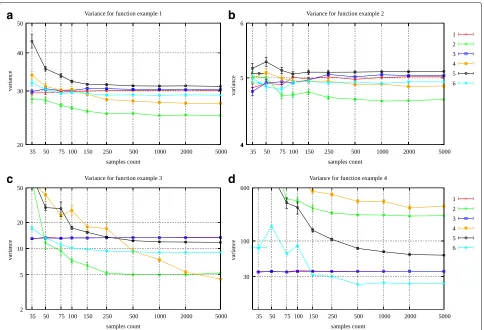
Fig. 1From left to right and from top to bottom: The four functions (in black) used in the four examples,f1(x)(example 1),f2(x)(example 2),f3(x)

(example 3),f4(x)(example 4), as combination of the three functionsx(red),x2−x/π(green), andsin(x)(blue)

• The heuristically based estimators for unbiased techniques defined in [9] and [10] give better results than the one defined in Section6for possibly biased techniques, except for the third example, where the new heuristic performs much better.

• We obtain in one case an acceleration of more than 30 times over the variance of the balance heuristic estimator with equal count of samples.

Table 2Variances for multi-sample estimator for the four examples in AppendixCand the environment map example (×10−3) for balance heuristic using equal count of samples, for the count inversely proportional to the variances of independent estimators [9] and [10], for the provably better, non-balance heuristic, estimator defined in [11], and for the three new estimators defined in this paper

Ex. 1 Ex. 2 Ex. 3 Ex. 4 Ex. EM

αk∝1_n 29.16 4.91 10.68 28.14 4.63

αk∝_vk1 [9,10] 24.11 4.55 2.02 330.85 1.47

αk∝σk,eq[11] 29.09 4.90 10.61 27.94 4.61

αk∝_m12

k

26.55 4.77 0.37 809.28 3.16

αk∝σk,eq 29.90 4.99 9.48 6.61 4.36

αk∝Mk,eq 28.24 4.83 7.05 18.04 3.87

7.2 Adaptive results for 1D functions

We present also results for the four 1D examples computed with adaptive sampling algorithms. A first batch using equal number of samples from each tech-nique computes order 1 approximation of the different quantities, which in turn allows us to obtain a first approximation of the α values needed for the second batch. The samples of batch N + 1 are obtained with the orderN approximation of the α values, and incre-mentally update the N-order quantities. We provide in supplemental material the C++ code to compute all estimators adaptively. The pseudo-code for the estimators

Table 3Variances for one-sample balance heuristic for the four examples in AppendixCand the environment map example (×10−3_{) for balance heuristic using equal count of samples, for} the count inversely proportional to the variances of independent estimators [9] and [10], and for the three new estimators defined in this paper

Ex. 1 Ex. 2 Ex. 3 Ex. 4 Ex. EM

αk∝1_n 30.16 5.02 13.35 35.16 5.14

αk∝vk1 [9,10] 24.22 4.60 2.05 332.97 1.50

αk∝_m12

k

27.04 4.85 0.39 863.50 3.46

αk∝σk,eq 31.03 5.10 11.67 57.38 4.84

Table 4Variance times cost (i.e., inefficiency, the smaller the better) for multi-sample estimator for the four examples in AppendixC and the environment map example (×10−3) for balance heuristic using equal count of samples, for the count inversely proportional to the variances of independent estimators [9] and[10], for the provably better, non-balance heuristic, estimator defined in [11], and for the three new estimators defined in this paper

Example 1 Example 2 Example 3 Example 4 Example EM

αk∝1n 102.26 17.24 37.47 98.68 13.41

αk∝ckvk1 [9,10] 40.41 9.28 4.03 300.12 1.31

αk∝σ√k,eqck [11] 89.40 15.44 31.80 83.78 11.31

αk∝_ckm12

k

43.06 9.82 3.12 534.37 1.68

αk∝σ√k,eq_ck 81.43 13.54 28.68 91.01 5.88

αk∝Mk√,eq_ck 79.73 13.08 25.74 31.77 4.92

defined in [9] and [10] can be found in the supplementary material of [10]. The charts with variances normalized to 1 sample, (i.e., variance times the number of samples), and variances times cost (i.e., inefficiencies) for specific costs as described in the Appendix C, and averaged for 100 runs are shown in Figs.2 and 3 for samples count from 35 to 5000.

7.3 2D analytical environment map example with Lafortune-Phong BRDF model

Let us consider here the BRDF formula for the physically based variant of the Phong model presented by Lafortune [27], assuming the case when the outgoing directionωois the surface normal:

fr(ωo,ωi)= ρ_πd +ρs

m+2 2π cos

m_{θ (56)}

whereρd is the diffuse albedo,ρsis the specular albedo,

m is the shininess, and θ is the angle between incident directionωiand the surface normal.

Let us consider also an environment map of intensity

R(ωi) = R·cosθ. As dω =sinθdθdφthe outgoing radi-ance is given then by the integral for the hemisphere in spherical parametrizationθ,φof the incident direction

R θ,φ

_ρ

d π +ρs

m+2 2π cos

m_{θ cosθcosθsinθdθdφ (57)}

and integrating overφwe get

2πR π/2

θ=0

_ρ

d π +ρs

m+2 2π cos

m_{θ cosθcosθsinθdθ. (58)}

By the variable substitution ofx=cosθ, we obtain

2πR

1

x=0

_ρ

d π +ρs

m+2 2π x

m _{x xdx. (59)}

We have thus the integral of the product p1(x)p2(x), wherep1(x)corresponds to the BRDF timesx=cosθ,

p1(x)=

_ρ

d π +ρs

m+2 2π x

m _{x, (60)}

andp2(x)=xis the environment map.

We used typical values,m = 5,ρ_d = ρs = 0.5, and compared for equal cost and for the empirically obtained sampling costs,c1 = 1,c2 = 4.8. The detailed results are in the last columns of Tables2,3,4,5, and in the last two columns of Table6. The results confirm the patterns found in our 1D examples.

8 Conclusions

This paper discussed an important topic of MIS esti-mators and the limited acceleration over equal count of

Table 5Variance times cost (i.e., inefficiency, the smaller the better) for one-sample estimator for the four examples in AppendixCand the environment map example (×10−3_{) for balance heuristic using equal count of samples, for the count inversely proportional to the} variances of independent estimators [9] and[10], and for the three new estimators defined in this paper

Example 1 Example 2 Example 3 Example 4 Example EM

αk∝1n 105.78 17.60 46.82 123.30 14.90

αk∝ckvk1 [9,10] 40.89 9.37 4.04 300.48 1.32

αk∝_ckm12

k

44.43 9.93 3.18 545.53 2.30

αk∝σ√k,eqck 83.82 13.27 33.36 105.80 6.39

Table 6αj_i:αivalues for thej-th 1D example and for the environment map example

Example 1 Example 2 Example 3 Example 4 Example EM

α1

1 α21 α31 α12 α22 α23 α31 α23 α33 α14 α42 α43 α1 α2 α=1

n 0.33 0.33 0.33 0.33 0.33 0.33 0.33 0.33 0.33 0.33 0.33 0.33 0.5 0.5

αk∝_vk1 [9,10] 0.42 0.48 0.10 0.35 0.21 0.44 0.90 0.10 0.00 0.95 0.04 0.00 0.93 0.07

αk∝ckvk1 [9,10] 0.79 0.14 0.06 0.68 0.07 0.25 0.98 0.02 0.00 0.99 0.01 0.00 0.99 0.01

αk∝σk,eq[11] 0.33 0.31 0.35 0.34 0.34 0.31 0.37 0.32 0.30 0.37 0.32 0.30 0.52 0.48 αk∝σ√k,eq_ck [11] 0.51 0.19 0.29 0.52 0.21 0.26 0.55 0.19 0.25 0.55 0.19 0.25 0.70 0.30

αk∝_m12

k

0.38 0.39 0.23 0.35 0.29 0.36 0.53 0.46 0.01 0.60 0.36 0.04 0.66 0.34

αk∝_ckm12

k

0.52 0.16 0.32 0.69 0.09 0.22 0.87 0.12 0.00 0.56 0.19 0.25 0.90 0.10

αk∝Mk,eq 0.33 0.35 0.30 0.32 0.31 0.35 0.34 0.36 0.28 0.33 0.32 0.34 0.57 0.43 αk∝Mk√,eqck 0.52 0.21 0.25 0.50 0.19 0.30 0.52 0.22 0.24 0.50 0.19 0.29 0.75 0.25

samples balance heuristic. We have shown that in reality, this bound on acceleration does not hold, which justifies the search for better and more efficient estimators. We have obtained, both without and with taking into account the cost of sampling, new balance heuristic estimators

that are provably better than balance heuristic with equal count of samples, and new heuristic estimators valid even when the independent techniques are biased. We have analyzed their behavior with 1D examples and with a 2D environment map example.

a

b

c

d

a

c

b

d

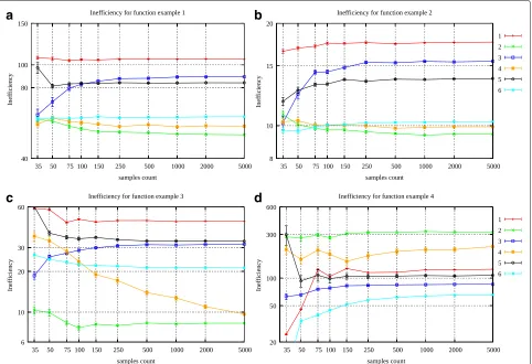
Fig. 3The inefficiency for the estimators for adaptive sampling for different samples count and specific costs of sampling techniques for examples in AppendixC.aExample 1,bexample 2,cexample 3, anddexample 4. Notation of lines 1 to 6 in charts follows the order of rows in Table4

Appendix A: Inequality in Theorem 9.5 of Veach’s thesis does not hold for balance heuristic

Let us repeat first the proof of Eq.24such as it appears in Veach’s thesis

V[F] = n

i=1 1

Ni

_w2

i(x)f2(x)

pi(x)

dx−μ2_i

(61)

≥ n

i=1 1

N

w2_i(x)f2(x) pi(x)

dx−μ2_i

= 1

n

n

i=1 1

N/n

w2_i(x)f2(x) pi(x)

dx−μ2_i

= 1

nV[Feq] ,

where V[Feq] is computed assuming the same weights as V[F] but with equal count of samples. Let us see that inequality61does not hold when the weightswi(x) depend on theNi. We will see it for the balance heuristic estimator, where the weights are defined by

wi(x)=

Nipi(x)

n

k=1Nkpk(x)

. (62)

Eq.61would be

V[Fˆ] = n

i=n 1

Ni

N_i2f2(x)pi(x)

n

k=1Nkpk(x)

2dx−μ 2 i

≥ n

i=1 1

N

N_i2f2(x)pi(x)

n

k=1Nkpk(x)

2dx−μ 2 i

= 1

n

n

i=1 1

N/n

_N2

if2(x)pi(x)

n

k=1Nkpk(x)

2dx−μ 2 i

= 1

N

n

i=1

f2(x)pi(x)

n

k=1pk(x)

2dx−μ2i

= 1

nV

ˆ

Feq

, (63)

as the last but two expression is clearly not the variance of a balance heuristic estimator with equal count of samples (Eq.16). Inequality61thus holds only when the weights

Appendix B: Section 5 proofs

We present the proof of Theorem2. This proof is similar to the proof of Theorem2in [11].

ProofTo optimize the varianceVFˆ1₌n i=1α1iM

2 i − μ2_{, we use Lagrange multipliers with the constraint}

n

Computing the partial derivatives and equating them to zero, as theMido not depend on theαi, we get αj ∝ Mj. The Hessian matrix, obtained with the second derivatives of V[Fˆ1_{], is a diagonal matrix with positive} diagonal values

and thus is positive-definite. The variance function is then strictly convex in its convex domainn_i=1αi = 1, where for alli, 0 < αi < 1, meaning that the critical point is unique and a minimum.

Substituting the optimal values, i.e.,αj∝Mj, we find the minimum variance,

ProofLet us considercithe cost of sampling with tech-nique i. The average cost (or cost for one total sample) is thus CT =

iαici. We want to minimize now the cost times variance, i.e.,CT×VF1, which is the inverse

of efficiency. We use Lagrange multipliers with the con-straintn_i=1αi=1 and objective function

Taking partial derivatives and equating them to zero, as theMido not depend on theαi,

Multiplying byαjand adding overj, we obtain

n we find that the optimal sampling counts are the ones in Eq.49.

We present here the proof of Theorem4.

ProofWe compare first the efficiency of the general one-sample MIS estimator with weights given by Eq.14

andαi ∝Mi,eq/√ci, with the balance heuristic estimator with equal count of samples. The inverse of efficiency, i.e., cost times variance, is given in both cases by Eq.70:

_n

Let us compare first the terms corresponding to the

sec-ond moments, i.e., the termn_i=1αici ni=1 M2

i,eq αi , for

inequality, we can easily check that Eq.71is true, where

Let us consider now the term of Eq.70that containsμ2_, i.e.,n_i=1αici

μ2_{. Whenever theα}

ivalues are decreasing withci, the following inequality can be proved [26,28].

Thus, we can guarantee that the general MIS estimator with weightswi(x)given by Eq.14andαi ∝Mi,eq/√ciis more efficient than the one-sample balance heuristic esti-mator with equal count of samples whenever theαivalues are decreasing withci. Considering now the one-sample balance heuristic estimator withαi ∝ Mi,eq/√ci, as the costs are the same and the variance is less than the gen-eral MIS estimator considered by virtue of Theorem 9.4 in Veach’s thesis, its efficiency is higher, and in turn, higher than the balance heuristic estimator with equal count of sampling.

Appendix C: 1D examples

We compare the results for the functions and pdfs in Fig.1

with the following estimators: equal count of samples, count inversely proportional to variances of independent techniques [9], the new heuristic defined in Section 6

of this paper, optimal count in [11], and the two new balance heuristic provably better estimators defined in Sections4and5. These two new estimators are tried for both one-sample and multi-sample.

Example 1

Suppose we want to solve the integral

μ=I= respectively. We first find the normalization constants:

π 1.89. We take into account the sampling costs given in [9], i.e.,c1 = 1,c2 = 6.24,c3 = 3.28.

Example 2

Let us solve the integral

μ = I =

As the third example, let us solve the integral

μ =I =

using the same functions as before.

Example 4

As the last example, consider the integral of the sum of the three pdfs

In this case, we know the optimal (zero variance)α val-ues:(0.3, 0.3, 0.4). This case should be most favorable to equal count of samples.

Results are summarized in Tables2,3,4,5, and 6.

Acknowledgements

The authors acknowledge the comments by anonymous reviewers that helped to improve a preliminary version of the paper.

Funding

The authors are funded in part by Czech Science Foundation research program GA14-19213S by grant TIN2016-75866-C3-3-R from the Spanish Government and by grant OTKA K-124124 and VKSZ-14 PET/MRI 7T.

Authors’ contributions

Equal contribution from all authors. All authors read and approved the final manuscript.

Competing interests

The authors declare that they have no competing interests.

Publisher’s Note

Springer Nature remains neutral with regard to jurisdictional claims in published maps and institutional affiliations.

Author details

1_{School of Computer Science and Technology, Tianjin University, Tianjin,}

China.2_{Department of Informatics, Applied Mathematics and Statistics,}

University of Girona, Campus de Montilivi, Girona, Spain.3_{Czech Technical}

University at Prague, Faculty of Electrical Engineering, Prague, Czech Republic.

4_{Budapest Technical University, Budapest, Hungary.}

Received: 11 July 2017 Accepted: 23 January 2018

References

1. E Veach, LJ Guibas, inProceedings of the 22nd Annual Conference on Computer Graphics and Interactive Techniques. SIGGRAPH ’95. Optimally Combining Sampling Techniques for Monte Carlo Rendering (ACM, New York, 1995), pp. 419–428.https://doi.org/10.1145/218380.218498.http:// doi.acm.org/10.1145/218380.218498

2. E Veach, Robust Monte Carlo Methods for light transport simulation. PhD thesis, Stanford University (1997)

3. V Elvira, L Martino, D Luengo, MF Bugallo, Efficient multiple importance sampling estimators. IEEE Signal Process. Lett.22(10), 1757–1761 (2015). https://doi.org/10.1109/LSP.2015.2432078

5. K Subr, D Nowrouzezahrai, W Jarosz, J Kautz, K Mitchell, Error analysis of estimators that use combinations of stochastic sampling strategies for direct illumination. Comput. Graph. Forum Proc. EGSR.33(4), 93–102 (2014).https://doi.org/10.1111/cgf.12416

6. M Pharr, G Humphreys,Physically based rendering, Second Edition: From Theory To Implementation, 2nd edn. (Morgan Kaufmann Publishers Inc., San Francisco, 2010)

7. H Lu, R Pacanowski, X Granier, Second-order approximation for variance reduction in multiple importance sampling. Comput. Graph. Forum. 32(7), 131–136 (2013).https://doi.org/10.1111/cgf.12220

8. A Pajot, L Barthe, M Paulin, P Poulin, Representativity for robust and adaptive multiple importance sampling. IEEE Trans. Vis. Comput. Graph. 17(8), 1108–1121 (2011).https://doi.org/10.1109/TVCG.2010.230 9. V Havran, M Sbert, inProceedings of the 13th ACM SIGGRAPH International

Conference on Virtual-Reality Continuum and Its Applications in Industry, VRCAI ’14. Optimal Combination of Techniques in Multiple Importance Sampling (ACM, New York, 2014), pp. 141–150.https://doi.org/10.1145/ 2670473.2670496.http://doi.acm.org/10.1145/2670473.2670496 10. M Sbert, V Havran, Adaptive multiple importance sampling for general

functions. Vis. Comput. 1–11 (2017). https://doi.org/10.1007/s00371-017-1398-1

11. M Sbert, V Havran, L Szirmay-Kalos, Variance analysis of multi-sample and one-sample multiple importance sampling. Comput. Graph. Forum. 35(7), 451–460 (2016).https://doi.org/10.1111/cgf.13042

12. GO Roberts, A Gelman, WR Gilks, Weak convergence and optimal scaling of random walk Metropolis algorithms. Ann. Appl. Probab.7, 110–120 (1997)

13. C Andrieu, J Thoms, A tutorial on adaptive MCMC. Stat. Comput.18(4), 343–373 (2008)

14. T Hachisuka, HW Jensen, Robust adaptive photon tracing using photon path visibility. ACM Trans. Graph.30(5), 114–111411 (2011).https://doi. org/10.1145/2019627.2019633

15. L Szirmay-Kalos, L Szécsi, Improved stratification for metropolis light transport. Comput. Graph.68(Supplement C), 11–20 (2017).https://doi. org/10.1016/j.cag.2017.07.032

16. T Hachisuka, AS Kaplanyan, C Dachsbacher, Multiplexed metropolis light transport. ACM Trans. Graph.33(4), 100–110010 (2014).https://doi.org/ 10.1145/2601097.2601138

17. A Owen, Y Zhou, Safe and Effective Importance Sampling. J. Am. Stat. Assoc.95, 135–143 (2000)

18. R Douc, A Guillin, J-M Marin, CP Robert, Convergence of Adaptive Mixtures of Importance Sampling Schemes. Ann. Stat.35(1), 420–448 (2007).https://doi.org/10.1214/009053606000001154

19. R Douc, A Guillin, JM Marin, CP Robert, Minimum variance importance sampling via population monte carlo. ESAIM: Probab. Stat.11, 424–447 (2007)

20. J-M Cornuet, J-M Marin, A Mira, CP Robert, Adaptive multiple importance sampling. Scand. J. Stat.39(4), 798–812 (2012).https://doi.org/10.1111/j. 1467-9469.2011.00756.x

21. J-M Marin, P Pudlo, M Sedki, Consistency of the adaptive multiple importance sampling. Preprint arXiv:1211.2548 (2012).http://arxiv.org/ abs/1211.2548

22. L Martino, V Elvira, D Luengo, J Corander, An adaptive population importance sampler: Learning from uncertainty. IEEE Trans. Signal Process. 63(16), 4422–4437 (2015).https://doi.org/10.1109/TSP.2015.2440215 23. V Elvira, L Martino, D Luengo, J Corander, inProceedings of ICASSP 2015. A

gradient adaptive population importance sampler (IEEE, Brisbane, 2015), pp. 4075–4079

24. V Elvira, L Martino, D Luengo, MF Bugallo, Efficient multiple importance sampling estimators. IEEE Signal Process. Lett.22(10), 1757–1761 (2015). https://doi.org/10.1109/LSP.2015.2432078

25. GH Hardy, JE Littlewood, G Pólya,Inequalities. (Cambridge University Press, Cambridge, 1952)

26. M Sbert, J Poch, A necessary and sufficient condition for the inequality of generalized weighted means. J. Inequalities Appl.2016(1), 292 (2016). https://doi.org/10.1186/s13660-016-1233-7

27. EP Lafortune, YD Willems, Using the modified Phong reflectance model for physically based rendering. Technical Report report CW197, Dept. of Computer Science, K.U.Leuven (1994)