R E S E A R C H
Open Access
Computable performance guarantees for
compressed sensing matrices
Myung Cho
*, Kumar Vijay Mishra and Weiyu Xu
Abstract
The null space condition for1minimization in compressed sensing is a necessary and sufficient condition on the sensing matrices under which a sparse signal can be uniquely recovered from the observation data via1
minimization. However, verifying the null space condition is known to be computationally challenging. Most of the existing methods can provide only upper and lower bounds on the proportion parameter that characterizes the null space condition. In this paper, we propose new polynomial-time algorithms to establish upper bounds of the proportion parameter. We leverage on these techniques to find upper bounds and further develop a new procedure—tree search algorithm—that is able to precisely and quickly verify the null space condition. Numerical experiments show that the execution speed and accuracy of the results obtained from our methods far exceed those of the previous methods which rely on linear programming (LP) relaxation and semidefinite programming (SDP).
Keywords: Compressed sensing, Null space condition,1minimization , Performance guarantee, Sensing matrix
1 Introduction
Compressed sensing is an efficient signal processing tech-nique to recover a sparse signal from fewer samples than required by the Nyquist-Shannon theorem, reducing time and energy spent in sampling operation. These advan-tages make compressed sensing attractive in various signal processing areas [1].
In compressed sensing, we are interested in recovering the sparsest vectorx ∈ Rnthat satisfies the underdeter-mined equationy=Ax. Here,Ris the set of real numbers, A∈Rm×n, m<nis a sensing matrix, andy∈Rmis the observation or measurement data. This is posed as an0 minimization problem:
minimizex0
subject toy=Ax, (1)
wherex0is the number of non-zero elements in vector x. The0minimization is an NP-hard problem. Therefore, we often relax (1) to its closest convex approximation—the
1minimization problem: minimizex1
subject toy=Ax. (2)
*Correspondence:[email protected]
Department of ECE, University of Iowa, Iowa City, IA, 52242, USA
It has been shown that the optimal solution of0 min-imization can be obtained by solving 1 minimization under certain conditions (e.g., restricted isometry prop-erty or RIP) [2–6]. For random sensing matrices, these conditions hold with high probability. We note that RIP is a sufficient condition for sparse recovery [7].
A necessary and sufficient condition under which a k-sparse signalx, (k n) can be uniquely obtained via1 minimization is null space condition (NSC) [3, 8, 9]. A matrixAsatisfies NSC for a positive integerkif
||zK||1<||zK||1 (3)
holds true for allz ∈ {z : Az = 0,z = 0} and for all subsetsK⊆ {1, 2,. . .,n}with|K| ≤k. Here,Kis an index set,|K|is the cardinality ofK,zK is the part of the vectorz over the index setK, andKis the complement ofK. NSC is related to the proportion parameterαkdefined as
αk maximize
{z:Az=0,z=0}maximize{K:|K|≤k} zK1
z1
. (4)
Theαkis the optimal value of the following optimization problem:
maximize z,{K:|K|≤k} zK1
subject toz1≤1, Az=0, (5)
whereKis a subset of{1, 2,. . .,n}with cardinality at most k. The matrixAsatisfies NSC for a positive integerkif and only ifαk< 12. Equivalently, NSC can be verified by com-puting or estimatingαk. The role ofαk is also important in the recovery of an approximately sparse signalxvia1 minimization where a smallerαkimplies more robustness [8–10].
We are interested in computingαkand, especially, find-ing the maximum k for whichαk < 12. However, com-putingαk to verify NSC is extremely expensive and was reported in [7] to be NP-hard. Due to the challenges in computingαk, verifying NSC explicitly for determin-istic sensing matrices remains a relatively unexamined research area. In [3, 8, 11, 12], convex relaxations were used to establish upper or lower bounds of αk (or other parameters related toαk) instead of computing the exact αk. While [3, 11] proposed semidefinite programming-based methods, [8, 12] suggested linear programming relaxations to obtain the upper and lower bounds ofαk. For both methods, computable performance guarantees on sparse signal recovery were reported via boundingαk. However, these bounds ofαk could only verify NSC with k=O(√n), even though theoretically,kcan grow linearly withn.
Our work drastically departs from these prior meth-ods [3,8,11,12] that provide only the upper and lower bounds. In our solution, we propose the pick-l-element algorithms (1 ≤ l < k), which compute upper bounds of αk in polynomial time. Subsequently, we leverage on these algorithms to develop the tree search algo-rithm (TSA)—a new method to compute an exact αk by significantly reducing computational complexity of an exhaustive search method. This algorithm offers a way to control a smooth trade-off between complexity and accu-racy of the computations. In the conference precursor to this paper, we had introducedsandwiching algorithm (SWA) [13], which employs a branch-and-bound method. Although SWA can also be used to calculate the exactαk, it has a disadvantage of greater memory usage than TSA. On the other hand, TSA provides memory and perfor-mance benefits for high-dimensional matrices (e.g., up to size∼6000×6000).
It is noteworthy that our methods are different from RIP or the neighborly polytope framework for analyzing the sparse recovery capability of random sensing matri-ces. For example, prior works such as [6,22] employ the neighborly polytope to predict theoretical lower bounds on recoverable sparsity k for a randomly chosen Gaus-sian matrix. However, our methods do not resort to a probabilistic analysis and are applicable for any given deterministic sensing matrix. Also, our algorithms have the strength of providing better bounds than existing methods [3, 8, 11, 12] for a wide range of matrix sizes.
1.1 Main contributions
We summarize our main contributions as follows:
(i) Faster algorithms for high dimensions. We designed the pick-l algorithm (and its optimized version), wherel is a chosen integer, to provide upper bounds onαk. We are able to show that whenl increases, the optimized pick-l algorithm provides tighter upper bound onαk. Numerical experiments show that, even withl=2or 3, the pick-l algorithm already provides better bound onαkthan the previous algorithms based on the LP [8] and SDP [3]. For large sensing matrices, the pick-1-element algorithm can be significantly faster than the LP and SDP methods. (ii) Novel formulations using branch-and-bound. Based on the pick-l algorithm, we propose a branch-and-bound tree search approach to compute tighter bounds or even the exact value ofαk. To the best of our knowledge, this tree search algorithm is the first branch-and-bound algorithm to verify NSC for1 minimization. This branch-and-bound approach heavily depends on the pick-l algorithm developed in this paper. For example, the LP [8] and SDP [3] methods cannot be directly adapted to provide an efficient branch and bound approach, due to their lack of subset-specific upper bounds onαk. In numerical experiments, we demonstrated that the tree search algorithm reduced the execution time to precisely calculateαkby around 40–8000 times, compared to the exhaustive search method.
(iii) Simultaneous upper and lower bounds. The branch-and-bound tree search algorithm simultaneously maintains upper and lower bounds ofαkduring the run-time. This approach has two benefits. Firstly, if one is interested in merely certifying the NSC for a positivek rather than obtaining the exactαk, then one can terminate the TSA early to shorten the running time. This can be done as soon as the global upper (lower) bound drops below (exceeds) 1/2 and, therefore, concluding that the NSC for the positivek is satisfied (not satisfied). Secondly, consider the case when TSA is terminated early due to, say, constraints on running time. Then, the process still yields meaningful bounds onαkvia the record of continuously maintained upper and lower bounds. (iv) New results on recoverable sparsity. For a certain
1.2 Notations and preliminaries
We denote the sets of real numbers and positive integers asRandZ+respectively. We reserve uppercase lettersK andLfor index sets and lowercase lettersk,l ∈ Z+for their respective cardinalities. We also use| · |to denote the cardinality of a set. We assumek > l ≥ 1 through-out the paper. For vectors or scalars, we use lowercase letters, e.g.,x,k,l. For a vectorx ∈ Rn, we usexi for its i-th element. If we use an index set as a subscript of a vector, it represents the partial vector over the index set. For example, whenx∈ RnandK = {1, 2},xK represents [x1,x2]T. We reserve uppercase A for a sensing matrix whose dimension ism×n. Since the number of columns of a sensing matrixAisn, the full index set we consider is{1, 2,. . .,n}. In addition, we representnlnumbers of solution of an optimization problem. For instance,z∗and K∗are the optimal solution of (5). Since we need to rep-resent an optimal solution for each index setLi, we use the superscripti∗to represent an optimal solution for an index setLi, e.g.,zi∗. The maximum value ofksuch that bothαk < 12 andαk+1 ≥ 12 hold true is denoted by the maximum recoverable sparsity kmax.
2 Pick-l-element algorithm
Consider a sensing matrix withncolumns. Then, there are nk subsets K each of cardinality k. When n and k are large, exhaustive search over these subsets to compute
αk is extremely expensive. For example, whenn = 100 andk = 10, it takes a search over 1.7310e+13 subsets to computeαk— a combinatorial task that is beyond the technological reach of common desktop computers. Our goal is to devise algorithms that can rapidly yield an exact value ofαk. As an initial step, we develop a method to compute an upper bound ofαkin polynomial time, which is called the pick-l-element algorithm (or simply, pick-l algorithm), wherelis a chosen integer such that 1≤l<k. Let us define the proportion parameter for a given index setLsuch that|L| =l, denoted byαl,L, as
(6) is the partial optimization problem of (4) only consid-ering the vectorzin the null space ofAfor a fixed index set L. We can obtainαl,Lby solving the following optimization problem:
maximize z zL1
subject toz1≤1, Az=0. (7)
Since (7) is maximizing a convex function for a given subsetL, we cast (7) as 2llinear programming problems by considering all the possible sign patterns of every element
ofzL(e.g., ifl=2 andL= {1, 2}, then,||zL||1= |z1| + |z2| can correspond to 2l = 4 possibilities:z1+z2,z1−z2,
−z1+z2, and −z1−z2).αl,L is equal to the maximum among the 2lobjective values.
The pick-lalgorithm usesαl,L’s obtained from different index sets to compute an upper bound ofαk. Algorithm 1 shows the steps of the pick-lalgorithm in detail. The fol-lowing Lemmata show that the pick-lalgorithm provides an upper bound of αk. Firstly, we provide Lemma 1 to derive the upper bound of the proportion parameter for a fixed index set K, and then, we show that the pick-l algorithm yields an upper bound ofαkin Lemma2.
Algorithm 1:Pick-l-element algorithm, 1 ≤ l < kfor computing an upper bound ofαk
1: Given a matrixA, calculateαl,L’s for all the subsetsL,
Lemma 1(Cheap Upper Bound (CUB) for a given sub-setK)Given a subset K, we have l}, we obtain the following inequality:
αk,K =
The inequality is from the optimal value of (6) for each index setLi.
where αl,L1 ≥αl,L2 ≥ · · · ≥αl,Li≥ · · · ≥αl,L(n l). (10)
ProofWithout loss of generality, we assume that when z=zi∗,i=1, 2,. . .,nl,αl,Li’s are obtained in descending
order like (10). It is noteworthy thatαk,K is defined for a fixedKset; however,αkis the maximum value over all the subsets with cardinalityk. Suppose that whenz=z∗and K = K∗,αk is achieved in (4). From the aforementioned definitions and similar argument as in Lemma1, we have:
αk =αk,K∗≤
The first inequality is from Lemma 1, and the last inequality is from the assumption thatαl,Li’s are sorted in
descending order.
The steps 2 and 3 in Algorithm 1, which are sortingαl,L’s and computing an upper bound ofαkwith sortedαl,L’s via (9), can also be done by solving the following optimization problem without sorting operation:
Here, we note that 1
(k−1
l. Therefore, for the
optimal value, the firstkllargest αl,Li’s are chosen with the coefficient 1
(k−1 l−1)
.
The upshot of the pick-lalgorithm is that we can reduce number of operations fromnkenumerations tonl. For example, whenn = 300,k = 20, andl = 2, the number of operations is reduced by around 1026 times. More-over, asnincreases, the reduction rate increases. With the reduced enumerations, we can still have non-trivial upper bounds ofαk through the pick-l-element algorithm. We will present the performance of the pick-l algorithm in Section5showing that the pick-lalgorithm provides bet-ter upper bounds than the previous research [3,8] even whenl =2. Furthermore, thanks to the pick-lalgorithm, we can design a new algorithm based on a branch-and-bound search to calculate αk by using upper bounds of αk obtained from the pick-l algorithm. It is notewor-thy that the cheap upper bound introduced in Lemma1 can provide upper bounds onαk,K for specific subsetsK, which enable our branch-and-bound method to calculate
αkor more precise bounds onαk. However, LP relaxation method [8] and SDP method [3] do not provide upper bounds onαk,K for specific subsetsK, which overwhelms LP and SDP methods to be used in the branch-and-bound method.
Since we are also interested in kmax, we introduce the following Lemma 3to bound the maximum recoverable sparsitykmax.
Lemma 3The maximum recoverable sparsity kmax sat-isfies
where.is the ceiling function.
Proof To prove this lemma, we will show that whenk=
l·1αl/2
−1,αk < 12. This can be concluded from the upper bound ofαkgiven as follows:
αk =αk,K∗≤
Note that there areklterms in the summation. From (13), if αl · kl < 12, then αk < 12. In other words, if k<l·1αl/2, thenαk< 12. Sincekis a positive integer, when k= l·1αl/2−1,αk< 12. Therefore, the maximum recov-erable sparsitykmaxshould be larger than or at least equal to l·1αl/2−1.
It is noteworthy that in ([8] Section 4.2.B), the authors introduced lower bound on k based on α1, i.e., k(α1). However, in Lemma3, we provide a more general result. Furthermore, in Lemma3, instead of usingαl, we can use an upper bound of αl to obtain the recoverable sparsity k; namely,k(UB(αl)) = l· UB1/(αl)2 −1 ≤ kmax, where UB(αl)represents an upper bound ofαl. Since the proof follows the same track as the proof of Lemma3, we omit the proof.
Finally, we introduce the following proposition to com-pare our algorithm to LP method [8] theoretically.
where ejis the standard basis vector with the j-th element equal to 1, and · k,1stands for the sum of k maximal magnitudes of components of a vector. Then we have:
αpick1
k ≥αkLP. (14)
For readability, we place the proof of Theorem 1 in Appendix A.
The LP method can provide tighter upper bounds onαk than the pick-1-element algorithm; however, this comes at a cost of solving a big optimization problem of design dimensionmn. Whenmandnare large, the complexity of computingαLPk can be prohibitive (please see Table2).
3 Optimized pick-lalgorithm
We can tighten the upper bound ofαk in the pick-l algo-rithm by replacing the constant factor 1
k−1
l−1
in (9) with
optimized coefficients at the cost of additional complexity, which we call as theoptimizedpick-lalgorithm. This opti-mized pick-lalgorithm is mostly useful from a theoretical perspective. In practice, it gives improved but similar per-formance in calculating the upper bound ofαkto the basic pick-lalgorithm described in Section2. As a theoretical merit of theoptimizedpick-lalgorithm, we can show that aslincreases, the upper bound ofαkbecomes smaller or stays the same.
The optimized pick-l algorithm provides an upper bound ofαkvia the following optimization problem:
maximize
In the following lemmata, we show that the optimized pick-lalgorithm produces an upper bound ofαkand this bound is tighter than that of the basic pick-l algorithm introduced in (11). The last lemma establishes that as l increases, the upper bound of αk decreases or stays the same.
Lemma 4The optimized pick-l algorithm provides an upper bound ofαk.
ProofThe strategy to prove Lemma 4 is to show that one feasible solution of (15) gives an upper bound ofαk. whether it satisfies the first and second constraints of (15). For the third constraint, let us check the case whenb=l first. Forb = l, we can choose an arbitrary index setB such that|B| = b = l. For the chosenB, there is only oneLi such thatB ⊆ Li, which is itself, i.e.,B = Li. For other chosenB’s, it is the same. Hence, the third constraint represents
Forb=1, the third constraint represents
=1, which satisfies (17). Basically,
the third constraint makes that for an index, the summa-tion of coefficients related to the index is limited to 1. In the same way, for 1 < b < l, the chosen γi is a feasi-ble solution of (15). From this feasible solution, we have
1
Lemma 5The optimized pick-l algorithm provides a tighter, or at least the same, upper bound ofαk than the basic pick-l algorithm introduced in (11).
ProofWe will show that the optimization problem (11) is a relaxation of (15). As in the proof of Lemma4, for b=l, the third constraint of (15) represents (16), which is involved in the first constraint of (11). Since the third con-straint of (15) considers otherbvalues such that 1≤b<l, (15) has more constraints than (11). Therefore, the opti-mized pick-l algorithm, which is (15), provides a tighter or at least the same upper bound than the basic pick-l algorithm.
ProofWe can upper bound the objective function of
Note that in the objective function of (18), each
αp,Pj, 1≤j≤
We can relax (18) to the following problem, which turns out to be the same as the optimized pick-palgorithm:
maximize
The relaxation is shown by checking the constraints. The first constraint of (19) is trivial to obtain. For the sec-ond constraint, we can obtain the secsec-ond constraint of (19) from the following relations:
(np)
where the second equality is obtained from the fact that
γi, which is a coefficient of αl,Li, appears deduced from the following inequality:
where the second equality is from the fact that for a fixed Pj, there are pick-palgorithm. Thus, whenl > p, the optimized pick-lalgorithm provides a tighter or at least the same upper bound than the optimized pick-palgorithm.
By using largerlin the pick-lalgorithm, we can obtain a tighter upper bound of αk. However, for a certain l, we need to enumeratenlpossibilities, and this becomes infeasible whenlis large. Moreover, whenl<k, the pick-l algorithm only gives an upper bound ofαk, instead of an exact value of αk. There is, however, a need to find tighter bounds onαk , or to even find the exact value of αk, whenkis too large for and-bound tree search algorithm to find tighter bounds onαkthan Lemma2provides, or to even find the exactαk. Our branch-and-bound tree search algorithm is enabled by the pick-lalgorithms introduced in Sections2and3.
4 Tree search algorithm
To find the index set K∗ which leads to the maximum
ofJ’s supersets, leading to reduced average-case computa-tional complexity. For simplicity, we will describe the TSA based on pick-1-element algorithm, simply called 1-Step TSA. However, we remark we can also extend the TSA to be based on pick-l-element (l ≥ 2) algorithm, by calcu-lating upper bounds of αk,K based on the results of the pick-l-element algorithm.
4.1 Tree structure
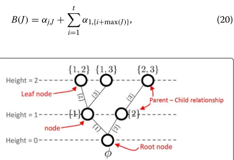
A tree nodeJrepresents an index subset of{1,. . .,n}such that|J| ≤k. We have the following rule:
[R1] A parent node is a subset of each of its child node(s).
A node that has no child is referred to as aleaf node. We call the cardinality of the index set corresponding to J asJ’sheight. The tree structure follows the “legitimate order,” which ensures that any new index in the child node is bigger than the indices of its parent node.
[R2] “Legitimate order” - LetP and C denote the parent node and the child node. Then, any index inP must be smaller than any index inC\P.
Figure1illustrates this rule in a tree withk = 2 and n=3.
4.2 Basic idea of a branch-and-bound approach for calculatingαk
We use a branch-and-bound approach over the tree struc-ture to calculateαk. This method maintains a lower bound onαk(how to maintain this lower bound will be explained in Section4.3). When the algorithm explores a tree node J, the algorithm calculates an upper boundB(J), which is no smaller thanαk,K for any child nodeK(with cardinal-ityk) of nodeJ. IfB(J)is smaller than the lower bound on
αk, then the algorithm will not explore the child nodes of the tree nodeJ.
In our algorithm, we calculateB(J)as
B(J)=αj,J + t
i=1
α1,{i+max(J)}, (20)
Fig. 1A tree structure following the legitimate order fork=2 and n=3
wherej+t =k, max(J)represents the largest index inJ, andα1,{1} ≥α1,{2}≥. . .≥α1,{n}. We obtain this descend-ing order by permutdescend-ing the columns of the sensdescend-ing matrix Ain descending order of α1,{i}’s as the pre-computation step of TSA. For example, in Fig.1, fork = 2,B({1}) =
α1,{1}+α1,{2}. In order to justify thatB(J)is an upper bound ofαk,K for all nodeK such thatJ ⊆ K, we provide the following lemma.
Lemma 7Givenα1,{1} ≥ α1,{2} ≥ . . . ≥ α1,{n}, B(J) =
αj,J+ti=1α1,{i+max(J)}, where j+t=k, and max(J) rep-resents the largest index in J, is an upper bound ofαk,K for all nodes K such that J⊆K .
ProofFor any subsetK such thatJ ⊆ K, we can write
αk,K = αj+t,{J∪T}, wherej+t = kandT = K\J. Then,
following exactly the same line of argument as in the proof of Lemma1, we have
αk,K ≤αj,J +αt,T,
and αt,T is no larger than jt∈Tα1,{j}. Finally, since α1,{i}’s are sorted in the descending order,j∈Tα1,{j} ≤
t
i=1α1,{i+max(J)}. Note that, due to the legitimate order [R2], the smallest element of the index setTis no less than 1+max(J). In conclusion, for all nodesKsuch thatJ⊆K, B(J)becomes an upper bound ofαk,K.
4.3 Best-first tree search strategy
TSA adopts a best-first tree search strategy for the branch-and-bound approach. We first describe a basic version of the best-first tree search strategy and then intro-duce two enhancements to this strategy in the next subsection.
In its basic version, TSA starts with a tree having only the root node and sets the global lower bound ofαkas 0. In each iteration, TSA selects a leaf tree nodeJwith the largestB(J)and expands the tree by adding the child nodes ofJto the tree. For each of these newly added child nodes, sayQ, TSA then calculates the upper boundB(Q)in (20). Note that if a newly added child nodeQhaskelements, TSA will calculateαk,Q,which is a lower bound onαk. For thisk-element Q, if the newly calculated αk,Q is bigger than the global lower bound ofαk, TSA will set the global lower bound equal toαk,Q. TSA will terminate if a leaf tree nodeJhas the largestB(J)among all the leaf nodes, and thatB(J)is no bigger than the global lower bound onαk.
4.4 Two enhancements
We incorporate two novel features to TSA in order to reduce the computational complexity. Firstly, when TSA attaches a new nodeQto a nodeJ in the tree structure, TSA computesB(Q)as (21):
B(Q)=αj,J+α1,Q\J+ t
i=1
α1,{i+max(Q)}, (21)
wherej+t+1=k, max(Q)represents the largest index in Q, andα1,{1}≥α1,{2} ≥. . .≥α1,{n}. Thus, without calcu-latingαj+1,Q (which involves higher computational com-plexity), we can still haveB(Q)as an upper bound ofαk,K for any child nodeK(with cardinalityk) of the nodeQ.
Secondly, when TSA adds a new nodeQas the child of nodeJin the tree structure (assumingαj,Jhas already been calculated), TSA does not need to add all ofJ’s child nodes to the tree at the same time. Instead, TSA only adds the nodeJ’s unattached child nodeQwith the largestB(Q)as defined in (21). Namely, the indexQ\Jis no bigger than the indexQ\J, whereQis any unattached child of the nodeJ. We note thatB(Q) is an upper bound onB(Q) (according to (21)) for any other unattached child nodeQ of the nodeJ. Thus, for any child nodeK(of cardinalityk) of nodeJ’s unattached child nodes,B(Q)is still an upper bound ofαk,K.
Algorithm 2 shows detailed steps of TSA, based on the pick-1-element algorithm (namely,l =1, 1-Step TSA). In the description, we define “expanding the tree from a node J” as follows:
Algorithm 2:Tree search algorithm based on the pick-1-element algorithm (1-Step TSA)
Input:A∈Rm×n,k,l←1 1-Step TSA, i.e.,l=1
Output: αk
Pre-computation:
1 computeαl,{i}fori=1,. . .,nvia (7)
2 permute columns ofAin descending order ofα1,{i}’s, so that
α1,{1}≥. . .≥α1,{n} Tree expansion:
3 start with root node∅, whereB(∅)=ki=1α1,{i}, in a tree structureϒ
4 Loop
5 J←a node that has the largestB(·)among all the leaf nodes in
ϒ
6 j← |J|
7 if αj,Jis not calculatedthen
8 computeαj,Jvia (7) and updateB(J)via (20)
9 expandϒfrom the parent ofJ See[R3] 10 else
11 ifj=kthen
12 αk←B(J)
13 break
14 else
15 expandϒfromJ See[R3]
16 end 17 end
18 EndLoop
[R3] “Expanding the tree from a nodeJ ”—attaching a new nodeQ to the node J, whereB(Q)is the largest value defined as (21) among the nodeJ ’s all the unattached child nodes.
4.5 Advantage of the tree search algorithm
Due to the nature of the branch-and-bound approach, we can obtain a global upper bound and a global lower bound of αk while TSA runs. As the number of itera-tions increases in TSA, we can obtain tighter and tighter upper bounds onαk, which is the largestB(·)among the leaf nodes. By using the global upper bound of αk, we can obtain a lower bound of the recoverable sparsitykvia Lemma3. Thus, even if the complexity of TSA is too high to finish in a timely manner, we can still obtain a lower bound on the recoverable sparsitykby early terminating TSA.
We note that the methods based on LP [8] and SDP [3] also provide upper bounds onαk. However, they are unable to determine upper bounds ofαk,K, which is for a specific index setK. This prevents the use of LP and SDP methods in our branch-and-bound method for computing
αk.
5 Numerical experiments
We conducted extensive simulations to computeαk and its upper/lower bounds using the pick-l algorithms and TSA. In this section, we call the pick-lalgorithms intro-duced in Section2and3as simply the (basic) pick-land the optimized pick-lalgorithms respectively.
For same matrices, we compared our methods with LP relaxation [8] approach and SDP method [3]. We assessed the computational complexity in terms of execution time of the algorithms.1In addition, we carried out numerical experiments to demonstrate the computational complex-ity of TSA empirically.
For LP method in [8] and SDP method in [3], we used the Matlab codes2 provided by the authors. Consistent with previous research, we used CVX [17]—a package for specifying and solving convex programs—for the SDP method, and MOSEK [18]—a commercial LP solver—for the LP method. In our own algorithms, we used MOSEK to solve (7). Also, to be consistent with the previous research, matrices were generated from the Matlab code provided by the authors of [3] athttp://www.di.ens.fr/~ aspremon/NSPcode.html. For valid bounds, we rounded down lower bounds onαk and exactαk, and rounded up upper bounds onαkto the nearest hundredth.
5.1 Performance comparison
5.1.1 Low-dimensional sensing matrices
Sensing matrices withn = 40 . We considered sens-ing matrices of row dimension m = 0.5n, 0.6n, 0.7n, 0.8n, wheren = 40. For every matrix size, we randomly generated 10 different realizations of Gaussian and par-tial Fourier matrices. So, in total we used 80 different n=40 sensing matrices for the numerical experiments in Tables 7 and 8. We normalized all of the matrix columns so that they have a unit2-norm. The entries of Gaussian matrices were i.i.d standard GaussianN(0, 1). The partial Fourier matrices hadmrows randomly draw from the full Fourier matrices. We compared our algorithms—pick-1-element, pick-2-algorithms—pick-1-element, pick-3-algorithms—pick-1-element, and TSA—to LP and SDP methods. For readability, we place the numerical results for these small sensing matrices in Appendix B.
For each matrix size and type, we increasedk from 1 to 5 in unit steps. Tables 7(a) and 8(a) show themedian values ofαk. (To be consistent with the previous research [3], in which the authors used the median value of αk to compare the SDP method with the LP method, we provided the median values obtained from 10 random realizations of sensing matrix.) From the median value of
αk, we obtained the recoverable sparsitykmax such that
αkmax <1/2 andαkmax+1>1/2. In addition, we calculated
the arithmetic mean ofkmax’s. For the arithmetic mean, we obtained eachkmaxfrom each random realization and computed the arithmetic mean of ten kmax’s. Compared with LP and SDP methods, we obtained bigger or at least the same recoverable sparsitykmaxby using pick-2, pick-3, and TSA. It is noteworthy that we obtained the exactαk fork=1, 2,. . ., 5 by using TSA, while LP and SDP meth-ods only provided the exactαk fork = 1. We observed thatαk < 1/2 but the upper bound ofαk > 1/2 holds true in several cases, e.g.,α5in 32×40 Gaussian matrices,
α4 in 28× 40 Gaussian matrices, α3 in 24×40 Gaus-sian matrices,α3in 20×40 partial Fourier matrices, and
α4in 24×40 partial Fourier matrices. Additionally, this can also be established by the arithmetic mean ofkmaxin Tables 7(a) and 8(a).
To compare the computational complexity, we calcu-lated the geometric mean of the algorithms’ execution time, to avoid biases for the average. Tables 7(b) and 8(b) list the average execution time. We also ran the exhaustive search method (ESM) to findαkand compared its execu-tion time with that of TSA. In calculatingα5, on average, 3-Step TSA reduced the computational time by around 86 times for 20×40 Gaussian matrices, and by 94 times for 20×40 partial Fourier matrices, compared to ESM. For 32×40 Gaussian matrix and partial Fourier matrix, the speedup compared to the bestl-Step TSA,l= 1, 2, 3, becomes around 1760 times and 182 times respectively. We observed that whenm/n= 0.5, e.g., 20×40 sensing matrices, in general, the 3-step TSA provides the fastest result fork = 5. On the other hand, form/n = 0.8 (e.g.,
32×40 case), the 2-Step TSA is the quickest in finding an exactαk fork = 5; however, fork > 5, the fastest l-step TSA cannot be determined from either experiments or theory.
Sensing matrices withn = 256 . We assessed the per-formance of the pick-l algorithm for sensing matrices with n = 256. We carried out numerical experiments on 128×256 Gaussian matrices in Fig.2aand 64×256 partial Fourier matrices in Fig. 2b. Here, for 10 sensing matrices, we obtained the median value of upper bounds ofαkusing the pick-lalgorithm and compared the result with LP relaxation method [8]. We omitted SDP method [3] from this experiment due to its very high computa-tional complexity. For the pick-3 algorithm in Fig.2a, we calculated an upper bound ofα3 via TSA and used this result to calculate upper bounds ofαk,k =3, 4,. . ., 8 via (13). Figure 2a,bdemonstrate that, with an appropriate choice ofl, the upper bound ofαkobtained via the pick-l algorithm can be tighter than that from the LP relaxation method. For example, for 128×256 Gaussian matrices, LP relaxation often determines the maximum recoverable sparsity as 5, while the pick-2 algorithm improves it to 6. In the pick-3 algorithm, the maximum recoverable spar-sity is 7 (α7=0.49). For 64×256 partial Fourier matrices, the maximum recoverable sparsity from LP relaxation and the pick-2 algorithm are 3 and 4 respectively.
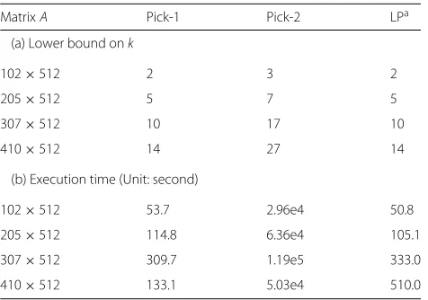
Sensing matrices withn=512 . We further conducted numerical experiments on Gaussian sensing matrices with n=512. The simulation results in Table1clearly demon-strate that the pick-2 algorithm provides larger lower bound on the recoverable sparsitykthan the LP method [8]. Especially, when Gaussian sensing matrix is 410×512, the lower bound onkobtained from the pick-2 algorithm is almost twice larger than that of the LP method.
5.1.2 High-dimensional sensing matrices
Fig. 2Median upper bounds ofαkfrom the pick-lalgorithm and the LP relaxation method.a128×256 Gaussian matricesb64×256 partial Fourier matrices
of LP method can be 10 times higher than our method on m×nGaussian matrices, wheremis large.
For extremely large sensing matrices, e.g, 4014×4096 and 6021×6144, the LP and SDP methods cannot provide any lower bound onkdue to unreasonable computational time. However, our pick-lalgorithm can still provide the lower bound on k efficiently. Table 3 shows the lower bound onkand the execution time for these large dimen-sional matrices, where our verified recoverable sparsityk can be as large as 558 for a 6134×6144 sensing matrix. We obtained the estimated time for the LP method by running the Matlab code obtained fromhttp://www2.isye. gatech.edu/~nemirovs/, which shows the percentage of the calculation on screen.
5.2 Comparison between the optimized pick-lalgorithm and the basic pick-lalgorithm
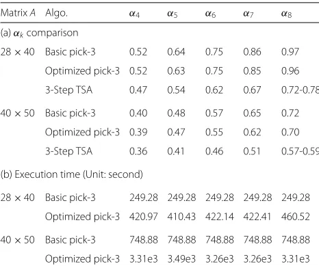
We compared the basic pick-l algorithm introduced in Section 2to the optimized pick-lalgorithm in Section3 on Gaussian sensing matrices 28 ×40 and 40 ×50 for l=3 andk=4, 5,. . ., 8. Table4demonstrates that when
Table 1Lower bound onkand execution time (Gaussian matrix withn=512)
MatrixA Pick-1 Pick-2 LPa
(a) Lower bound onk
102×512 2 3 2
205×512 5 7 5
307×512 10 17 10
410×512 14 27 14
(b) Execution time (Unit: second)
102×512 53.7 2.96e4 50.8
205×512 114.8 6.36e4 105.1
307×512 309.7 1.19e5 333.0
410×512 133.1 5.03e4 510.0
aLinear programming [8]
l = 3 andk = 4, 5,. . ., 8, the optimized pick-lalgorithm provided tighter upper bounds onαkthan the basic pick-l algorithm. This is because whenlis large andk > l, (15) includes more constraints, which leads to the reduced size of the feasible set, than the case whenkandlare small. Hence, the optimal value of (15), which is the result from the optimized pick-l, can be smaller than or equal to that of (11), which is the basic pick-l. Additionally, we provided the exactαk values obtained from TSA in order to check
Table 2Lower bound onkand execution time (Gaussian matrix withn=1024)
MatrixA Pick-1 kUB(α2)b k(α1) LPa
(a) Lower bound onk
102×1024 2 3 2 2
205×1024 4 4 4 4
307×1024 5 6 5 5
410×1024 7 8 7 7
512×1024 9 10 9 9
614×1024 12 13 12 12
717×1024 16 17 15 16
819×1024 21 23 20 21
922×1024 32 36 30 32
(b) Execution time (Unit: second)
102×1024 237 24 h 237 200
205×1024 452 24 h 452 429
307×1024 796 24 h 796 723
410×1024 1207 24 h 1207 1073
512×1024 1952 24 h 1952 1600
614×1024 2150 24 h 2150 2217
717×1024 1337 24 h 1337 2992
819×1024 838 24 h 838 3904
922×1024 386 24 h 386 4730
aLinear programming [8] bUpper bound ofα
Table 3Lower bound onkand execution time (Gaussian matrix)
MatrixA Pick-1 k(α1) LPa
(a) Lower bound onk
512×2048 7 6 7
2007×2048 102 90 102
4014×4096 152 139 N/Ab
1024×6144 8 8 8
6021×6144 190 174 N/A
6134×6144 558 406 N/A
(b) Execution time (Unit: second)
512×2048 7.51e3 7.51e3 6.63e3
2007×2048 6.71e2 6.71e2 7.19e4
4014×4096 9.12e3 9.12e3 15 daysc
1024×6144 2.18e5 2.18e5 1.61e5
6021×6144 3.89e4 3.89e4 65.5 daysd
6134×6144 1.37e4 1.37e4 41.7 dayse
aLinear programming [8] bNot available
cEstimated time (15 h for 4% calculations) dEstimated time (15 h for 1% calculations) eEstimated time (10 h for 1% calculations)
how tight the bounds obtained from the basic pick-land the optimized pick-lare. In terms of the execution time, the optimized pick-lalgorithm, which computes (15), was around 1.7 and 4.4 times slower than the basic pick-lon 28×40 and 40×50 Gaussian matrix respectively.
In summary, the optimized pick-l algorithm provides better or at least equal upper bound onαk to the basic pick-l algorithm, with additional complexity. In spite of
Table 4αkcomparison and execution time (Gaussian matrix)
MatrixA Algo. α4 α5 α6 α7 α8
(a)αkcomparison
28×40 Basic pick-3 0.52 0.64 0.75 0.86 0.97
Optimized pick-3 0.52 0.63 0.75 0.85 0.96
3-Step TSA 0.47 0.54 0.62 0.67 0.72-0.78
40×50 Basic pick-3 0.40 0.48 0.57 0.65 0.72
Optimized pick-3 0.39 0.47 0.55 0.62 0.70
3-Step TSA 0.36 0.41 0.46 0.51 0.57-0.59
(b) Execution time (Unit: second)
28×40 Basic pick-3 249.28 249.28 249.28 249.28 249.28
Optimized pick-3 420.97 410.43 422.14 422.41 460.52
40×50 Basic pick-3 748.88 748.88 748.88 748.88 748.88
Optimized pick-3 3.31e3 3.49e3 3.26e3 3.26e3 3.31e3
the increased complexity of the optimized pick-l algo-rithm, it has an important theoretical merit, which is Lemma6.
5.3 Complexity of tree search algorithm
In this subsection, we carried out numerical experiments to demonstrate the computational complexity of TSA empirically on randomly chosen Gaussian sensing matri-ces. Figure3a,bshows the distribution of execution time and the distribution of number of nodes in height 5 attached to the tree structure in TSA respectively. For m=0.5n, we generated 100 random realizations of Gaus-sian matrices and computed α5 using 3-Step TSA. The maximum number of leaf node whose cardinality iskis
n
k
= 40 5
= 6.58008e5. From Fig.3b, we note that for 90% of the cases, 3-Step TSA was terminated before 1.6% of all the possible height-5 nodes were attached to the tree structure.
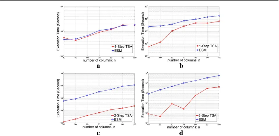
We provided the execution time of TSA for different-sized randomly chosen Gaussian matrices in Fig. 4. We compared the execution time of TSA to ESM. Figure4a shows that when k = 1, 1-Step TSA provides almost similar performance to ESM. This is because 1-Step TSA calculates all theα1,{i}’s as a pre-computation, which is the same procedure as ESM. However, for k > l as shown in Fig.4b–d, TSA can findαkwith reduced computation by using all theαl,L’s, while it is required to compute all theαk,K’s in ESM. In order to computeαk, we achieved a speedup of around 100 times via 2-Step TSA compared to ESM fork=3, 4.
In addition, in Fig.5, we compared the execution time of TSA to ESM by varyingkwithnfixed on random Gaus-sian matrices. For the best execution time of TSA, we used differentlvalues for TSA. Forn=40 andn=50, 3-Step TSA reduced the execution time to findα5by around 100 times and 300 times respectively, compared with ESM .
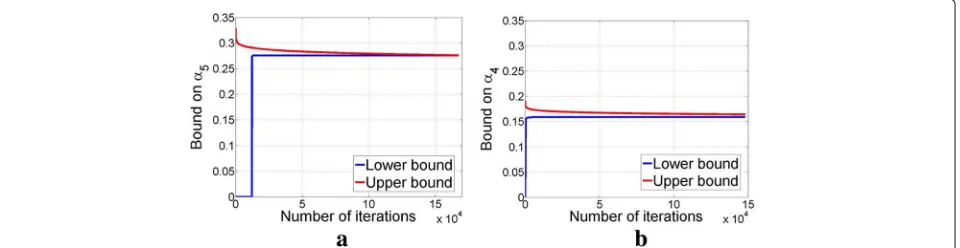
Finally, Fig. 6 gives illustrations of the values of the global lower and upper bounds, for 80×100 and 160×200 Gaussian sensing matrices, as the number of iterations in TSA increases. As we can see, the global upper and lower bounds get close very quickly. This implies that we can sometimes terminate TSA early and still obtain tight bounds onαk.
5.4 Application to network tomography problem
Fig. 3Histograms of the TSA (based on the pick-3 algorithm) to findα5on 100 randomly chosen 20×40 Gaussian sensing matrices for each method.aExecution time.bNumber of nodes in height 5
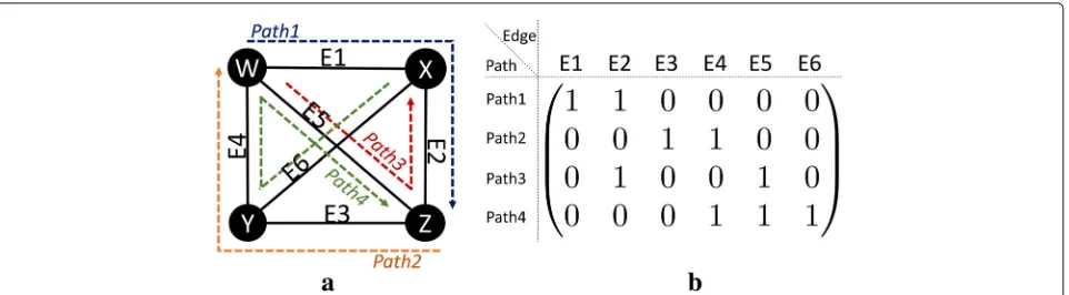
therefore, reasonable to think of finding the link delays as a sparse recovery problem. This sparse problem can be expressed in a system of linear equations y = Ax, where the vector y ∈ Rm is the delay of m paths, the vector x ∈ Rn is the delay vector for the n links, and A is a sensing matrix. The elementAij of Ais 1, if and only if pathyi, i ∈ {1, 2, . . ., m}, goes through linkj, j∈ {1, 2, . . ., n}; otherwise,Aijequal to 0 (see Fig.7). The indices of nonzero elements in the vectorxcorrespond to the congested links.
In our numerical experiments to verify NSC in network tomography problems, the paths for sending data packets were generated by random walks of fixed length. Table5 summarizes the results of our experiments. We note that
by using TSA, one canexactlyverify that a total ofk= 2 andk = 4 congested link delays can be uniquely found by solving1minimization problem (2) for the randomly generated network measurement matrices 33× 66 (12-node complete graph) and 53× 105 (15-node complete graph) respectively. For ESM, we estimated the execution time by multiplying the unit time to solve (7) and the total number of cases in the exhaustive search. We obtained the unit time to solve (7) by calculating the arithmetic mean from 100 trials. For a 53×105 matrix, 3-Step TSA sub-stantially reduced the execution time to find α5 around 137 times compared to ESM.
We further carried out numerical experiments on even larger network model having 300 nodes and 400 edges. We
Fig. 5The execution time of TSA in log scale as a function ofkon randomly chosenm×nGaussian matrices, wherem=n/2.an=40bn=50
created a random spanning tree for a network model by using random walk approach [24]. At each probing path, we randomly chose a node among 300 nodes as a start-ing point of random-walk and walked 100 times along the network connection. We obtained a 320×400 matrix cor-responding to the network model. We calculatedαkvalues vial-Step TSA, wherel = 1, 2. In terms of the execu-tion time, in Table6, we compared TSA with ESM, where the unit time to solve (7) was obtained by calculating the arithmetic mean from 100 trials. Especially, 1-Step TSA reduced the execution time to findα4by around 28,700 times compared to ESM.
5.5 Discussion
In this section, we discuss the strengths and weaknesses of our proposed algorithms, compared with earlier research [3,8].
1. Comparisons with LP and SDP. Our proposed pick-1-element algorithm can achieve similar performance as the LP [8] and SDP methods [3]. However, our pick-1-element algorithm has the clear advantage of being more computationally efficient for large dimensional sensing matrices. Please see Table3, where the LP and SDP methods cannot provide the performance bounds on recoverable
sparsityk due to high computational complexity. On the other hand, in Table3, our pick-1-element algorithm can efficiently provide bounds on recoverable sparsityk. The LP method has high computational complexity because it has to deal with a large convex program of design dimensionmn, which leads to prohibitive computational complexity whenm and n are large [8].
In our pick-1-element algorithm, we proposed the novel idea of sortingα1,{i}’s (see Lemma2), which leads to improved performance bounds onαkand recoverable sparsityk. This sorting idea, combined with Lemma2, provides us with larger recoverable sparsity boundk than purely usingα1for bounding recoverablek in ([8] Section 4.2.B).
2. Setspecific upper bounds. Our proposed pickl -element algorithm (l≥2) is novel and can provide improved bounds onαkand recoverable sparsityk, using polynomial computational complexity inn whenl is fixed. This approach is not practical when l is large. However, pick-2-element and pick-3-element algorithm can already provide improved performance bounds, compared with the previous research [3,8]. The fact that we can obtain upper bounds onαk, based on the results of pick-l -element (l≥2) algorithm, is new and non-trivial (see Lemma2,
Fig. 7 aA simple example of a network tomography graph.W,X,Y, andZare nodes in the network, andPath1, 2, 3, and 4 are the probing paths through which the packets are sent.bThe sensing matrix corresponding to the graph shown ina. The rows and columns of the matrix represent probing paths and edges respectively
Lemma3and Lemma4). For example, if we know α5≤0.22, we can use Lemma3to obtain that
α11≤0.22×11/5<0.5.
Our pick-l -element algorithm can provide set-specific upper bound forαk,K, laying the foundation for our branch-and-bound TSA. 3. Computational complexity of TSA. We proposed
TSA to find precise values forαkwith significantly reduced average-case computational complexity than
Table 5αkand execution time in network tomography problems
MatrixA Algo. α1 α2 α3 α4 α5 kmax
(a)αkvalues
33×66 1-Step TSA 0.28 0.41 0.50 0.57 0.62 2
2-Step TSA 0.28 0.41 0.50 0.57 0.62-0.64 2
3-Step TSA 0.28 0.41 0.50 0.57 0.62 2
53×105 1-Step TSA 0.20 0.29 0.36 0.45 0.52-0.54 4
2-Step TSA 0.20 0.29 0.36 0.45 0.49-0.56 4
3-Step TSA 0.20 0.29 0.36 0.45 0.52 4
(b) Execution time (Unit: second)
33×66 1-Step TSA 0.74 3.62 28.94 404.11 5.94e4
2-Step TSA 0.74 3.62 43.94 541.70 1 day
3-Step TSA 0.74 3.62 1.69e3 1.73e3 3.70e4
ESM 0.64 3.94 1.63e3 1.4e4a 1.8e5a
53×105 1-Step TSA 1.31 30.61 608.90 5.35e3 1 day
2-Step TSA 1.31 116.12 143.99 1.05e3 1 day
3-Step TSA 1.31 116.12 7.95e3 7.93e3 1.38e4
ESM 1.28 127.28 8.70.e3 9.6e4a 1.9e6a
Random walk step: 20
aExhaustive search method (estimated execution time = average time to solve (7) (=0.02 second) for an index set×total number of index sets)
ESM. The computational complexity of TSA is dependent onn, sparsity k, and a chosen constant l. Whenk, n, and l are large enough, findingαkvia TSA is still computationally expensive. In the worst case, TSA has the same computational complexity as ESM. However, our extensive simulations ranging from Fig.3to Fig.5and from Table5to Table8 show that on average, TSA can greatly reduce the computational complexity of findingαkcompared with ESM.
Moreover, since TSA maintains an upper bound and a lower bound ofαkduring its iterations, one can always early terminate TSA and still get improved performance bounds onαkthan the LP and SDP methods. We can use TSA to find an exact value of αl, wherel<k, and then use Lemma3to boundαk. 4. Use of data structures. We used object-oriented
programming (OOP) to implement TSA in Matlab [25], because the OOP makes it easy to handle tree-type structures. In OOP, we defined a class and
Table 6αkand execution time in a large network model having
300 nodes and 400 edges
Algo. α1 α2 α3 α4 α5 α6
(a)αkvalues
1-Step TSA 0.07 0.13 0.15 0.18 0.20 0.22-0.26a
2-Step TSA 0.07 0.13 0.15 0.18 0.20-0.23a 0.22-0.28a
(b) Execution time (Unit: second)
1-Step TSA 63.37 65.70 599.96 5.49e3 8.60e4 1 day
2-Step TSA 63.37 3.46e4 3.54e4 4.03e4 1 day 1 day
ESM 73.22 3.20e4 1.59e6b 1.58e8b 1.25e10b 8.22e11b
aLower bound - upper bound
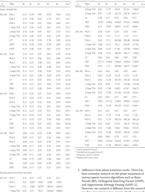
Table 7αkcomparison and execution time - Gaussian Matrix
A
(m×n) Algo. α1 α2 α3 α4 α5 kmax
d
(a)αkcomparison
20×40 Pick-1 0.28 0.55 0.81 1 1 1/1.1
Pick-2 0.28 0.45 0.66 0.85 1 2/1.9
Pick-3 0.28 0.45 0.57 0.76 0.92 2/1.9
1-Step TSA 0.28 0.45 0.57 0.67 0.75 2/1.9
2-Step TSA 0.28 0.45 0.57 0.67 0.75 2/1.9
3-Step TSA 0.28 0.45 0.57 0.67 0.75 2/1.9
LPa 0.28 0.50 0.67 0.84 0.98 2/1.6
SDPb 0.28 0.49 0.66 0.81 0.95 2/1.8
ESMc 0.28 0.45 0.57 0.67 0.75 2/1.9
24×40 Pick-1 0.23 0.46 0.67 0.87 1 2/2.0
Pick-2 0.23 0.37 0.53 0.69 0.85 2/2.1
Pick-3 0.23 0.37 0.46 0.61 0.75 3/2.8
1-Step TSA 0.23 0.37 0.46 0.57 0.65 3/2.8
2-Step TSA 0.23 0.37 0.46 0.57 0.65 3/2.8
3-Step TSA 0.23 0.37 0.46 0.57 0.65 3/2.8
LP 0.23 0.41 0.56 0.71 0.84 2/2.0
SDP 0.23 0.41 0.55 0.70 0.82 2/2.0
ESM 0.23 0.37 0.46 0.57 0.65 3/2.8
28×40 Pick-1 0.18 0.36 0.53 0.70 0.86 2/2.0
Pick-2 0.18 0.31 0.46 0.59 0.72 3/3.0
Pick-3 0.18 0.31 0.41 0.54 0.66 3/3.0
1-Step TSA 0.18 0.31 0.41 0.49 0.57 4/3.5
2-Step TSA 0.18 0.31 0.41 0.49 0.57 4/3.5
3-Step TSA 0.18 0.31 0.41 0.49 0.57 4/3.5
LP 0.18 0.34 0.49 0.61 0.72 3/3.0
SDP 0.18 0.34 0.48 0.60 0.71 3/3.0
ESM 0.18 0.31 0.41 0.49 0.57 4/3.5
32×40 Pick-1 0.14 0.29 0.42 0.55 0.67 3/3.0
Pick-2 0.14 0.24 0.37 0.47 0.58 4/3.8
Pick-3 0.14 0.24 0.33 0.44 0.53 4/4.2
1-Step TSA 0.14 0.24 0.33 0.40 0.47 5/4.9
2-Step TSA 0.14 0.24 0.33 0.40 0.47 5/4.9
3-Step TSA 0.14 0.24 0.33 0.40 0.47 5/4.9
LP 0.14 0.27 0.38 0.49 0.58 4/3.9
SDP 0.14 0.27 0.38 0.48 0.57 4/4.0
ESM 0.14 0.24 0.33 0.40 0.47 5/4.9
(b) Execution time (Unit: second)
20×40 Pick-1 0.35 0.35 0.35 0.35 0.35
Pick-2 0.35 10.96 10.96 10.96 10.95
Pick-3 0.35 10.96 313.65 313.65 313.65
1-Step TSA 0.50 2.14 11.78 128.98 1.62e3
2-Step TSA 0.50 13.20 14.11 58.93 3.77e3
Table 7αkcomparison and execution time - Gaussian Matrix
(Continued)
A
(m×n) Algo. α1 α2 α3 α4 α5 kmax
d
3-Step TSA 0.50 13.20 320.20 346.43 695.53
LP 0.55 0.55 0.58 0.55 0.56
SDP 56.92 6.02e3 5.14e3 5.12e3 5.61e3
ESM 0.35 10.96 313.65 4.5e3 6.0e4
24×40 Pick-1 0.44 0.44 0.44 0.44 0.44
Pick-2 0.44 13.00 13.00 13.00 13.00
Pick-3 0.44 13.00 311.27 311.27 311.27
1-Step TSA 0.50 2.05 9.63 77.45 429.48
2-Step TSA 0.50 12.92 13.60 35.08 634.62
3-Step TSA 0.50 12.92 319.27 378.10 481.29
LP 0.84 0.94 0.88 0.83 0.82
SDP 62.18 5.59e3 4.89e3 4.75e3 5.37e3
ESM 0.44 13.00 311.27 4.6e3 6.4e4
28×40 Pick-1 0.58 0.58 0.58 0.58 0.58
Pick-2 0.58 14.67 14.67 14.67 14.67
Pick-3 0.58 14.67 326.80 326.80 326.80
1-Stpe TSA 0.52 1.41 4.39 32.43 119.86
2-Stpe TSA 0.52 13.54 13.82 29.35 126.62
3-Stpe TSA 0.52 13.54 327.79 404.23 383.61
LP 1.12 1.20 1.12 1.09 0.68
SDP 71.27 5.55e3 4.90e3 4.98e3 4.72e3
ESM 0.58 14.67 326.80 4.7e3 6.9e4
32×40 Pick-1 0.42 0.42 0.42 0.42 0.42
Pick-2 0.42 13.29 13.29 13.29 13.29
Pick-3 0.42 13.29 331.80 331.80 331.80
1-Step TSA 0.55 1.14 2.89 13.50 40.67
2-Step TSA 0.55 14.22 14.32 18.13 40.35
3-Step TSA 0.55 14.22 340.87 336.29 355.06
LP 0.70 0.71 0.72 0.70 0.70
SDP 56.12 7.17e3 5.43e3 5.07e3 4.79e3
ESM 0.42 13.29 331.80 4.9e3 7.1e4
aLinear programming [8] bSemidefinite programming [3] cExhaustive search method dMedian/arithmetic mean
Table 8αkcomparison and execution time - Partial Fourier
Matrix
A
(m×n) Algo. α1 α2 α3 α4 α5 kmax
d
(a)αkcomparison
20×40 Pick-1 0.19 0.39 0.59 0.78 0.98 2/2.0
Pick-2 0.19 0.36 0.55 0.73 0.91 2/2.2
Pick-3 0.19 0.36 0.47 0.64 0.80 3/2.7
1-Step TSA 0.19 0.36 0.47 0.61 0.70 3/2.7
2-Step TSA 0.19 0.36 0.47 0.61 0.70 3/2.7
3-Step TSA 0.19 0.36 0.47 0.61 0.70 3/2.7
LPa 0.19 0.39 0.59 0.78 0.98 2/2.0
SDPb 0.19 0.39 0.59 0.78 0.98 2/2.0
ESMc 0.19 0.36 0.47 0.61 0.70 3/2.7
24×40 Pick-1 0.15 0.31 0.47 0.62 0.78 3/2.8
Pick-2 0.15 0.27 0.42 0.55 0.69 3/3.0
Pick-3 0.15 0.27 0.38 0.51 0.64 3/3.4
1-Step TSA 0.15 0.27 0.38 0.49 0.59 4/3.5
2-Step TSA 0.15 0.27 0.38 0.49 0.59 4/3.5
3-Step TSA 0.15 0.27 0.38 0.49 0.59 4/3.5
LP 0.15 0.31 0.47 0.62 0.78 3/2.8
SDP 0.15 0.31 0.47 0.62 0.78 3/2.8
ESM 0.15 0.27 0.38 0.49 0.59 4/3.5
28×40 Pick-1 0.12 0.25 0.37 0.50 0.62 4/3.6
Pick-2 0.12 0.23 0.35 0.47 0.58 4/4.0
Pick-3 0.12 0.23 0.32 0.44 0.54 4/4.0
1-Step TSA 0.12 0.23 0.32 0.41 0.50 4/4.0
2-Step TSA 0.12 0.23 0.32 0.41 0.50 4/4.1
3-Step TSA 0.12 0.23 0.32 0.41 0.50 4/4.1
LP 0.12 0.25 0.37 0.50 0.62 4/3.6
SDP 0.12 0.25 0.37 0.50 0.62 4/3.6
ESM 0.12 0.23 0.32 0.41 0.50 4/4.1
32×40 Pick-1 0.09 0.19 0.29 0.38 0.48 5/4.7
Pick-2 0.09 0.17 0.27 0.36 0.44 5/4.7
Pick-3 0.09 0.17 0.25 0.35 0.43 5/4.7
1-Step TSA 0.09 0.17 0.25 0.33 0.39 5/4.7
2-Step TSA 0.09 0.17 0.25 0.33 0.39 5/4.7
3-Step TSA 0.09 0.17 0.25 0.33 0.39 5/4.7
LP 0.09 0.19 0.29 0.38 0.48 5/4.7
SDP 0.09 0.19 0.29 0.38 0.48 5/4.7
ESM 0.09 0.17 0.25 0.37 0.39 5/4.7
(b) Execution time (Unit: second)
20×40 Pick-1 0.31 0.31 0.31 0.31 0.31
Pick-2 0.31 10.85 10.85 10.85 10.85
Pick-3 0.31 10.85 260.41 260.41 260.41
1-Step TSA 0.47 9.72 70.57 329.28 3.60e3
Table 8αkcomparison and execution time - Partial Fourier
Matrix (Continued)
A
(m×n) Algo. α1 α2 α3 α4 α5 kmax
d
2-Step TSA 0.47 11.97 18.54 45.18 3.36e3
3-Step TSA 0.47 11.97 291.29 297.45 633.12
LP 0.49 0.77 0.53 0.59 0.51
SDP 33.93 2.34e3 2.65e3 2.91e3 2.60e3
ESM 0.31 10.85 260.41 4.1e3 6.0e4
24×40 Pick-1 0.39 0.39 0.39 0.39 0.39
Pick-2 0.39 11.51 11.51 11.51 11.51
Pick-3 0.39 11.51 302.86 302.86 302.86
1-Step TSA 0.48 12.12 76.21 407.67 2.77e3
2-Step TSA 0.48 12.52 21.46 107.00 1.83e3
3-Step TSA 0.48 12.52 306.43 426.17 1.36e3
LP 0.62 0.56 0.66 0.59 0.58
SDP 41.13 2.39e3 2.66e3 2.63e3 2.56e3
ESM 0.39 11.51 302.86 4.5e3 6.4e4
28×40 Pick-1 0.43 0.43 0.43 0.43 0.43
Pick-2 0.43 13.29 13.29 13.29 13.29
Pick-3 0.43 13.29 341.05 341.05 341.05
1-Step TSA 0.50 8.70 31.53 272.68 731.90
2-Step TSA 0.50 12.99 16.85 47.45 544.79
3-Step TSA 0.50 12.99 317.40 410.47 553.67
LP 0.65 0.67 0.71 0.67 0.75
SDP 40.51 2.17e3 2.29e3 2.80e3 2.63e3
ESM 0.43 13.29 341.05 4.7e3 6.5e4
32×40 Pick-1 0.57 0.57 0.57 0.57 0.57
Pick-2 0.57 17.24 17.24 17.24 17.24
Pick-3 0.57 17.24 385.26 385.26 385.26
1-Step TSA 0.52 6.39 22.35 101.67 451.62
2-Step TSA 0.52 13.38 18.65 49.46 372.35
3-Step TSA 0.52 13.38 326.40 476.55 1.02e3
LP 0.86 0.89 0.78 0.75 0.76
SDP 46.51 2.41e3 2.62e3 2.53e3 2.75e3
ESM 0.57 17.24 385.26 4.8e3 6.8e4
aLinear programming [8] bSemidefinite programming [3] cExhaustive search method dMedian/arithmetic mean
and the previous works [3,8] are focusing on worst-case performance guarantee (recovering all the possiblek -sparse signals), while the research on phase transition is considering the average-case performance guarantee for a singlek -sparse signal with fixed support and sign pattern. Secondly, the phase transition bounds are mostly for random matrices. Hence, for a given deterministic sensing matrix, phase transition results cannot be used for that particular matrix.
6 Conclusion
In this paper, we consider the problem of verifying the null space condition in compressed sensing. Calculat-ing the proportional parameter αk that characterizes the null space condition of a sensing matrix is a non-convex optimization problem, and also known to be NP-hard in [7]. In order to verify the null space condi-tion, we proposed novel and simple enumeration-based algorithms, which are called the basic and optimized pick-l algorithms, to obtain upper bounds of αk. With these algorithms, we further designed a new algorithm called the tree search algorithm to gain a global solu-tion to the non-convex optimizasolu-tion problem of veri-fying the null space condition. Numerical experiments show that our algorithms outperform the previously proposed algorithms [3, 8] in performance as well as speed.
Endnotes
1We conducted our experiments on HP Z220 CMT
with Intel Core i7-3770 dual core CPU @3.4GHz clock speed and 16GB DDR3 RAM, using Matlab (R2013b) on Windows 7.
2LP method from http://www2.isye.gatech.edu/~
nemirovs/and SDP method fromhttp://www.di.ens.fr/~ aspremon/NSPcode.html.
Appendix
Proof of proposition1
ProofLet us denote the sum ofkmaximal magnitudes of elements ofx∈Rnas kdistinct integers between 1 andn. For a matrix, sayA, we useAi,jto represent its element in thei-th row andj-th
where we can exchange the order of “maximize” and “min-imize” in the last equality because ||eit −ATyit||∞ only
depends onyit.
Moreover, according to the equations for “αi” between (4.29) and (4.30) in [8] (takingβthere to be∞), upper bound calculated by Lemma2(based on the pick-1-element algorithm). Namely,
αLP
k ≤α
pick1
k . (23)
Sensing matrices withn=40
Here, we provide the numerical results for small sensing matrices withn = 40 to compare our methods to LP [8] and SDP [3] methods.
Acknowledgements
We thank Alexandre d’Aspremont from CNRS at Ecole Normale Superieure, Anatoli Juditsky from Laboratoire, Jean Kuntzmann at Universite Grenoble Alpes, and Arkadi Nemirovski from Georgia Institute of Technology for helpful discussions and providing codes for the simulations in [3] and [8].
Funding
The work of Weiyu Xu is supported by Simons Foundation 318608, KAUST OCRF-2014-CRG-3, NSF DMS-1418737, and NIH 1R01EB020665-01.
Availability of data and material
All the codes used for the numerical experiments are available at the following link:https://sites.google.com/view/myungcho/software/nsc.
Authors’ contributions
Competing interests
The authors declare that they have no competing interests.
Publisher’s Note
Springer Nature remains neutral with regard to jurisdictional claims in published maps and institutional affiliations.
Received: 23 December 2016 Accepted: 7 February 2018
References
1. YC Eldar, G Kutyniok,Compressed Sensing: Theory and Applications. (Cambridge University Press, Cambridge, 2012)
2. EJ Candès, T Tao, Decoding by linear programming. IEEE Trans. Inf. Theory.51(12), 4203–4215 (2005)
3. A d’Aspremont, L El Ghaoui, Testing the nullspace property using semidefinite programming. Math. Prog.127(1), 123–144 (2011) 4. EJ Candès, J Romberg, T Tao, Robust uncertainty principles: exact signal
reconstruction from highly incomplete frequency information. IEEE Trans. Inf. Theory.52(2), 489–509 (2006)
5. EJ Candès, J Romberg, T Tao, Stable signal recovery from incomplete and inaccurate measurements. Comm. Pure Appl. Math.59(8), 1207–1223 (2006)
6. D Donoho,Neighborly polytopes and sparse solution of underdetermined linear equations. Technical report. (Stanford University. Dept of Statistics, Stanford, 2005)
7. AM Tillmann, ME Pfetsch, The computational complexity of the restricted isometry property, the nullspace property, and related concepts in compressed sensing. IEEE Trans. Inf. Theory.60(2), 1248–1259 (2014) 8. A Juditsky, A Nemirovski, On verifiable sufficient conditions for sparse
signal recovery via1minimization. Math. Prog.127(1), 57–88 (2011)
9. A Cohen, W Dahmen, R DeVore, Compressed sensing and bestk-term approximation. J. American Math. Soc.22(1), 211–231 (2009) 10. W Xu, B Hassibi, Precise stability phase transitions for1minimization: a
unified geometric framework. IEEE Trans. Inf. Theory.57(10), 6894–6919 (2011)
11. K Lee, Y Bresler, inProceedings of IEEE International Conference on Acoustics, Speech and Signal Processing (ICASSP). Computing performance guarantees for compressed sensing, (2008), pp. 5129–5132 12. G Tang, A Nehorai, inProceedings of Conference on Information Sciences
and Systems (CISS). Verifiable and computable∞performance evaluation of1sparse signal recovery, (2011), pp. 1–6
13. M Cho, W Xu, inProceedings of Asilomar Conference on Signals, Systems and Computers. New algorithms for verifying the null space conditions in compressed sensing, (2013), pp. 1038–1042
14. W Xu, E Mallada, A Tang, inProceedings of IEEE International Conference on Computer Communizations (INFOCOM). Compressive sensing over graphs, (2011), pp. 2087–2095
15. MH Firooz, S Roy, inProceedings of IEEE Global Telecommunications Conference (GLOBECOM). Network tomography via compressed sensing, (2010), pp. 1–5
16. MJ Coates, RD Nowak, inProceedings of IEEE International Conference on Acoustics, Speech, and Signal Processing (ICASSP). Network tomography for internal delay estimation, vol.6, (2001), pp. 3409–3412
17. M Grant, S Boyd, CVX: Matlab software for disciplined convex programming, version 2.1 beta (2012).http://cvxr.com/cvx 18. MOSEK ApS, The MOSEK optimization toolbox for MATLAB manual.
Version 7.1 (Revision 31) (2015).http://docs.mosek.com/7.1/toolbox/ index.html
19. Y Tsang, M Coates, RD Nowak, Network delay tomography. IEEE Trans. Signal Process.51(8), 2125–2136 (2003)
20. Y Vardi, Network tomography: estimating source-destination traffic intensities from link data. J. American Stat. Assoc.91(433), 365–377 (1996) 21. R Castro, M Coates, G Liang, R Nowak, B Yu, Network tomography: recent
developments. Stat. Sci.19(3), 499–517 (2004)
22. DL Donoho, J Tanner, Precise undersampling theorems. Proc. IEEE.98(6), 913–924 (2010)
23. G Brassard, P Bratley,Fundamentals of algorithmics. (Englewood Cliffs, Prentice Hall, 1996)
24. DB Wilson, inProceedings of the twenty-eighth annual ACM symposium on Theory of computing. Generating random spanning trees more quickly than the cover time, (1996), pp. 296–303