R E S E A R C H
Open Access
Fast dictionary learning from incomplete
data
Valeriya Naumova
1*and Karin Schnass
2Abstract
This paper extends the recently proposed and theoretically justified iterative thresholding andKresidual means (ITKrM) algorithm to learning dictionaries from incomplete/masked training data (ITKrMM). It further adapts the algorithm to the presence of a low-rank component in the data and provides a strategy for recovering this low-rank component again from incomplete data. Several synthetic experiments show the advantages of incorporating information about the corruption into the algorithm. Further experiments on image data confirm the importance of considering a low-rank component in the data and show that the algorithm compares favourably to its closest dictionary learning counterparts, wKSVD and BPFA, either in terms of computational complexity or in terms of consistency between the dictionaries learned from corrupted and uncorrupted data. To further confirm the
appropriateness of the learned dictionaries, we explore an application to sparsity-based image inpainting. There the ITKrMM dictionaries show a similar performance to other learned dictionaries like wKSVD and BPFA and a superior performance to other algorithms based on pre-defined/analytic dictionaries.
Keywords: Dictionary learning, Sparse coding, Sparse component analysis, Thresholding, K-means, Erasures, Masked data, Corrupted data, Inpainting
1 Introduction
Many notable advances in modern signal processing are based on the fact that even high-dimensional data fol-lows a low complexity model. One such model, which has become an important prior for many signal processing tasks ranging from denoising and compressed sensing to super resolution, inpainting and classification, is sparsity in a dictionary [1–8]. In the sparse model, each datum (signal) can be approximated by the linear combination of a small (sparse) number of elementary signals, called atoms, from a pre-specified basis or frame, called dictio-nary. In mathematical terms, if we represent each signal by a vectoryn ∈ Rdand collect the entire dataset in the matrixY =(y1,. . .,yN)∈Rd×N, the sparse model can be formalised as
Y =XandXis sparse. (1)
Here, the dictionary matrixcontainsKnormalised vec-tors (atoms)φk, stored as columns in=(φ1,. . .,φK)∈
*Correspondence:[email protected]
1Simula Metropolitan Center for Digital Engineering, Martin Linges 25, 1325 Fornebu, Norway
Full list of author information is available at the end of the article
Rd×K, and each vector columnx
n ∈ RK of the matrix
X = (x1,. . .,xN) ∈ RK×N contains only few non-zero entries. Since the model expressed in Eq. (1) has proven to be very useful in signal processing, the natural next question is how to automatically learn a dictionary , providing sparse representations for a given data class. This problem is also known as dictionary learning, sparse coding or sparse component analysis. By now, there exist not only a multitude of dictionary learning algorithms to choose from [9–16] but also theoretical results have started to accumulate [17–26]. As our reference list is nec-essarily incomplete, we also point to the surveys [8,27] as trailheads for algorithms and theory respectively.
One common assumption on which all algorithms and associated theories are based is that large numbers of clean signals are available for learning the dictionary. However, this assumption might not be valid in actual applications. Therefore, in this paper, we consider the following problem: How do we learn a dictionary when there are only a few or no clean training signals avail-able? This problem naturally arises in various application domains from environmental surveillance, health care to automotive manufacturing, where the data of interest are
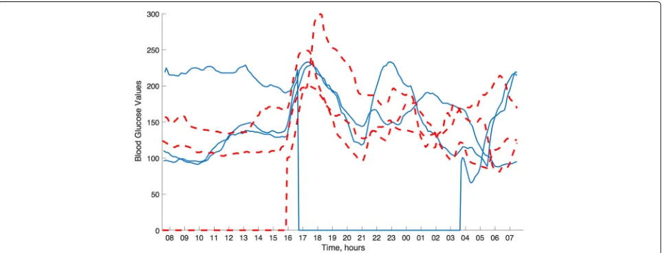
measured by sensors. As signals from sensors can often be incomplete or contain erroneous measurements due to sensor dropouts or need for recalibration respectively, the amount of clean and reliable data for performing predictive tasks becomes a real issue. As an illustrative example, in Fig.1, we provide examples of blood glucose traces from two patients as measured by a commercially available continuous glucose monitoring sensor. One can observe that, despite mandatory calibration procedures of the device several times a day, the device quite often returns obviously wrong, e.g. rapidly oscillating, estima-tions of the blood glucose level and suffers from frequent signal dropouts [28].
To solve the problem of learning from incomplete data, we propose an algorithm calledIterative Thresholding and
K residual Means for Masked data (ITKrMM). As the
name suggests, it is built upon the inclusion of a sig-nal corruption model into the theoretically-justified and numerically efficientIterative Thresholding and K residual Means(ITKrM) algorithm [29].
In order to model the data corruption/loss process, we adapt the concept of the binary erasure channel. In this model, the measurement device sends a value and the receiver either receives the value or receives a message that the value was not received (‘erased’). The model is used frequently in information theory due to its simplic-ity and its abstraction towards modelling various types of data losses. At the same time, this setting provides infor-mation on the location of the erasures and, thus, we can employ the concept of a maskMto describe the corrupted data asMy. Without loss of generality, we will think of a maskMas orthogonal projection onto the linear span of vectors from the standard basis(ej)j or simply as diago-nal matrix with M(j,j) ∈ {0, 1}. We further extend the
algorithm to account for the presence of a low-rank com-ponent in the data. Such comcom-ponents appear in many real-life signals and, as we will illustrate below, should be treated cautiously in the considered context.
To evaluate the accuracy and efficiency of the algo-rithm, we perform various numerical tests on synthetic and image data. We also confirm the appropriateness of the learned dictionaries by successfully using them for an image inpainting task.
The dictionary learning community does not directly address the problem under consideration. However, dic-tionaries learned or refined from corrupted data appear in the image processing community, where they, among other tasks, are used for inpainting. Examples include weighted KSVD (wKSVD) [30, 31], an adaption of the KSVD algorithm to handling non-homogenous noise in signals as well as missing values, and the Beta-Bernoulli Process Factor Analysis (BPFA) [32], a parameter free Bayesian algorithm, that learns dictionaries for inpaint-ing also from corrupted data. As we will see, the main advantage of ITKrMM over the wKSVD algorithm is a significant reduction of computational cost, from around 3.5 h to 18 min in our experiments on image data, while providing similar approximation power and inpainting results. On the other hand, compared to BPFA, we observe similar computational complexity but a much higher con-sistency between the dictionaries learned from corrupted and uncorrupted data, which is also reflected in the bet-ter approximation power of the dictionary and inpainting performance, especially for middle and low corruption levels.
Contribution:This paper provides an efficient and sim-ple algorithm for dictionary learning from incomsim-plete data and the recovery of the low-rank component also
from incomplete data. Compared to its closest dictionary learning counterparts, wKSVD and BPFA, it combines the best of both worlds, meaning consistent and perfor-mant dictionaries like wKSVD at the computational cost of BPFA.
Outline:The paper is organised as follows: Section2 contains the complete problem setup, explaining the com-bined low-rank and sparse model and as well as the corruption model. The ITKrMM algorithm for dictionary recovery is introduced in Section 3. An adaptation of this algorithm for recovery of the low-rank component from incomplete data together with a short discussion of related works in the field of matrix completion and dimen-sionality reduction is provided in Section4. Section5.1 contains extensive simulations on synthetic data, while in Section 5.2, we compare the learned dictionaries to those of wKSVD and BPFA for image data and use them for inpainting. Finally, Section6offers a snapshot of the main contributions and points out open questions and directions for future work.
Notation:Before finally lifting the anchor, we provide a short reminder of the standard notations used in this paper. For a matrix A, we denote its (conjugate) trans-pose byAand its Moore-Penrose pseudo inverse byA†. ByP(A), we denote the orthogonal projection onto the column span of A, i.e.P(A) = AA†, and by Q(A), the orthogonal projection onto the orthogonal complement of the column span ofA, that isQ(A)=Id−P(A), whereId is the identity operator (matrix) inRd.
The restriction of the dictionaryto the atoms indexed by I is denoted by I, i.e.I = (φi1,. . .,φiS), ij ∈ I.
The maximal absolute inner product between two differ-ent atoms is called the coherenceμof a dictionary,μ = maxk=j|
φk,φj
|, and encapsulates information about the local dictionary geometry.
2 Problem setup
Our goal is to learn a dictionaryfrom corrupted signals
Mnyn, under the assumption that the signalsynare sparse in the dictionary. There are some notable differences in this problem setting compared to the uncorrupted sit-uation. First, we cannot without loss of generality assume that the corrupted signals are normalised, since the action of the mask distorts the signal energy,My2 ≤ y2, which makes simple renormalisation impossible.
Another issue in modelling a natural phenomenon is that the signals might not be perfectly sparse but can only be modelled as the orthogonal sum of low-rank and sparse components. An example for such signals are images, where one usually subtracts the foreground or, in other words, the signal mean before learning the dictio-nary, which consequently will consist of atoms with zero mean [9]. Without taking into account the existence of the low-rank component, one would likely end up with a
very ill-conditioned and coherent dictionary, where most atoms are distorted towards the low-rank component.
Similarly, in the example of the blood glucose data (see Fig. 1), we can observe that the signals vary around a baseline signal and that imposing a sparse structure in a dictionary makes sense only after subtracting this com-mon component. As before, the atoms in this dictionary should then be orthogonal to the baseline signal.
In the case of uncorrupted signals, one can simply deter-mine the common low-rank component = (γ1. . . γL) using one’s preferred method such as a singular value decomposition and subtract its contribution from the sig-nals viay˜n=Q()yn. Then, in a second separate step, one can run the dictionary learning algorithm on the modified signals y˜n and the resulting atoms will automatically be orthogonal to the low-rank component. However, in the case of corrupted signals, the action of the masks destroys the structure. So, while the dictionary is orthogonal to the low-rank component, = 0, this orthogonality is not preserved by the action of the mask, that isM = 0. As we will see later, the consequence of this effect is that we have to take the presence of the low-rank component into account when learning the sparsifying dictionary. Moreover, before even going to the dictionary learning phase, we have to find a strategy to recover the low-rank component from the corrupted signals.
dictionaries to signal reconstruction tasks such as inpaint-ing. There the information in the corrupted part of an image needs to be encoded by the rest of the image, which is the case if the image is sparsely represented by flat atoms.
Incorporating these considerations into the signal model previously used for the analysis of the ITKM algo-rithms [29], we arrive at the following model, which will be a foundation for the development and justification of the algorithm and for a future theoretical analysis.
2.1 Signal model and assumptions
Given ad×Llow-rank componentwith=ILand ad×K dictionary, where = 0 andL K, the signals are generated as
y=s·v+x+r
1+ r22
≈s(v+IxI), (2)
wherev22+ x22=1,|I| =S, andr=(r(1) . . .r(d))is a noise vector of a centred subgaussian random vector. The scaling parametersis distributed betweensminandsmax and accounts for signals with different energy levels.
The low-rank component is assumed to be present in every (most signals) and irreducible, meaning the coeffi-cientsvare dense andE(vv)is a diagonal matrix. Also, the average contribution of a low-rank atom should be larger than that of a sparse atom,E(|v()|) E(|x(k)|). At the same time, the size of the low-rank compo-nent is assumed to be much smaller than sparsity level, which in turn is much smaller than the signal dimension,
LSd.
The sparse coefficientsxshould be distributed in a way that for every single signal, onlyS entries inxare effec-tively non-zero. All atoms φk should be irreducible and on average contribute equally to the signals yn. Specifi-cally, no two atoms should always be used together, since in this case, they could be replaced by any other two atoms with the same span. For a more detailed discussion of admissible coefficient models, we refer to [29].
For those not intimately acquainted with dictionary learning, it might be helpful to keep in mind the follow-ing simple model for the subsequent derivations: constant scale and no noise. The low-rank component is one-dimensional, L = 1, and the low-rank coefficients are equally Bernoulli distributed±cv. The sparse coefficients are constructed by choosing a support I of size S uni-formly at random and setting x(k) = ±c, iid equally Bernoulli distributed, for k ∈ I and x(k) = 0 else. In other words, the coefficients restricted to the support are a scaled Rademacher sequence. Following the above con-siderations concerning the scalings, we havec2v+S·c2=1 andcv cS/K.
Similar to the signal model, we also discuss our corrup-tion model.
2.2 Corruption model and assumptions
As mentioned above, the corruption of a signalyis mod-elled by applying a mask M, where we assume that the distribution of the mask is independent of the signal dis-tribution. By receiving a corrupted signal, we understand that we have access both to the corrupted signalMyand the location of the corruption in form of the mask M, meaning we receive the pair(My,M).
For the development and later on testing of the algo-rithms, we will keep two types of corruption in mind. The first type are random erasures, where thejth coordinate is received with probabilityηjindependently of the recep-tion of the other coordinates, meaningM(j,j)∼B(ηj)are independent Bernoulli variables.
The second type are burst errors or sensor malfunc-tions. We model them by choosing a burst lengthτ and a burst startt, according to a distributionντ,t. Based onτ andt, we then setM(j,j)=0 fort≤j<t+τandM(j,j)=1 else. One simple realisation of such a distribution would be to have no burst,τ = 0, with probabilityθand a burst of fixed size, τ = T, which corresponds, for instance, to the time the sensor needs to be reset, with probability 1−θ. The burst start could be uniformly distributed, if the sensor is equally likely to malfunction throughout the measurement period or, for instance, with a higher weight on part of the coordinates, if the sensor is more likely to malfunction during part of the measurement period, for instance, during the night.
Having defined our problem setup, we are now ready to address the recovery of the dictionary from corrupted data.
3 Dictionary recovery
Algorithm 1(ITKrM - one iteration)Given an input dic-tionary , a sparsity level S and N training signals yn
do:
• For all n find Int =arg maxI:|I|=SIyn1. • For all k calculate
¯
To see how we have to modify the algorithm to deal with corrupted data, it will be helpful to understand how ITKrM works. ITKrM can be understood as fixed point iteration, meaning the generating dictionaryis a fixed point and locally, around the generating dictionary, one iteration of ITKrM is a contraction, φk− details, but for the sake of completeness, we provide some perhaps intuitive background for both the fixed point and the contraction property.
Assume for a moment that the signals follow the sim-plest sparse model, that is, they are perfectlyS-sparse in a generating dictionary, meaningyn = Inxn(In) for
some|In| =Sandxn(i)≈ ±cfori∈In, compared to the model presented in Section2. In particular, they all have the same scaling and contain neither a low-rank compo-nent nor are they contaminated by noise. If we are given the generating dictionary as input dictionary,=, then as long as the dictionary is not too coherent compared to the sparsity level,μ2S 1, thresholding will recover the generating support, meaningInt = In. Provided that the generating support was always recovered, we have
PIt n
yn =P(In)yn =ynand before normalisation the
updated atom takes the form
¯
This means that the output dictionary is again the gen-erating dictionary ¯ = or, in other words, that the generating dictionary is a fixed point of ITKrM. Note also that before normalisation, the updated atom consists of roughlyNk ={n:k∈In}scaled copies of itself because
To provide insight why one iteration of ITKrM acts as contraction, assume again that we know all generating
supportsIn and that our current estimate for the dictio-nary consists of all generating atoms except for the first one,ψk = φkfork ≥ 2. For the first atom, we only have some (poor) approximation, which is, however, still inco-herent with all other atoms, 1> | ψ1,φ1 | | ψ1,φk | ≈d−1/2fork≥2, or, in other words, the current estimate ψ1contains more of the first than of any other generating atom. As before, one iteration of ITKrM will preserve all atomsψk = φk fork ≥ 2 and on top of that contractψ1 towardsφ1. To see this, observe that as long as the current estimate contains more of the first than of any other gen-erating atoms,| ψ1,φ1 | | ψ1,φk |, whenever 1 ∈ I
Combining the two estimates and noting that sign(ψ1yn)=xn(1), we get
which shows that also, a poor approximation of ψ¯1 is quickly contracted towards the generating atomφ1.
In summary, for our modifications, we have to ensure that both the fixed point and the contraction prop-erty are preserved. To start with, we again assume that the corrupted signals have equal scale, contain no low-rank component, and are not contaminated by noise but are perfectly S-sparse, that is Mnyn = MnInxn(In).
First, observe that a corrupted signalMnyn is not sparse in the generating dictionary but in its corrupted versionMn,
Mnyn=MnInxn(In)=
i∈In
xn(i)Mnφi.
destroyed, Mnφk = 0, or perfectly preserved, Mnφk = φk. Therefore, the proper dictionary representation of the corrupted signal is
and in order to recover the support In via threshold-ing, we have to look at the inner products between the corrupted signal and the renormalised non-vanishing cor-rupted atoms,
Looking back at the representation of a corrupted sig-nal in the properly scaled corrupted dictionary (4), we can also see why we assume flatness of the dictionary atoms, i.e. φk∞ 1 for allk. In the ideal case where for all the dynamic range of the corrupted signal with respect to the corrupted normalised dictionary is the same as the original dynamic range,
maxi∈In|x(i)| · Mnφi2
mini∈In|x(i)| · Mnφi2
= maxi∈In|x(i)|
mini∈In|x(i)|
However, the less equally distributed over the coor-dinates the energy of the undamaged atoms is, the more the energy of the corrupted atoms varies. This leads to an increase of the dynamic range, which in turn makes it harder for thresholding to recover the generating support.
The second reason for assuming flat atoms is the increase in coherence caused by the corruption. If the coherence of two flat atoms is small, this means that their inner product is a sum of many small terms with different signs eventually almost cancelling each other out. Such a sum is quite robust under (random) era-sures, since both negative and positive terms are erased. On the other hand, if the energy of two atoms is less uniformly distributed, small coherence might be due to one larger entry in the sum being cancelled out by many small entries. Thus, the erasure of one large entry can cause a large increase in coherence, which again
decreases the chances of thresholding recovering the gen-erating support.
Finally, to see that the flatness assumption is not merely necessary due to the imperfection of the thresholding algorithm for sparse recovery, assume that the atoms of the generating dictionary are combinations of two diracs φi=(δi−δ(i+1))/
√
2, that the coefficients follow our sim-ple sparse model and that the corruption takes the form of random erasures, i.e.Mn(j,j)are iid Bernoulli variables withP(Mn(j,j) = 0) = η. For large erasure probabilities, η >1/2, on average, about half of the maximally 2S non-zero entries of the signals will be erased and so the Dirac dictionaryψi =δior rather its erased version will provide as plausible anS-sparse representation to the corrupted signals as the original dictionary.
To see how to best modify the atom update rule, we first consider the case, where the corruption occurs always in the same locations, meaning Mn = M. Since we never observe the atoms on the coordinates where M(k,k) =
0, we can only expect to learn the corrupted dictionary
M = (Mφ1. . .Mφk) or rather its normalised version (Mφk/Mφk2). On the other hand, the problem reduces to a simple dictionary learning problem forMinstead of with update rule,
where we have used the fact that the projection onto a subdictionary is equal to the projection onto its nor-malised version and that signMψk,Myn
). Provided that thresholding always recov-ers the correct supportIn, we can conclude directly from above that the normalised corrupted dictionary will be a fixed point and that the update rule will contract towards it. Indeed, for any corruption pattern M, we know that before normalisation, an updated atomMψ¯k will be con-tracted towardsNk = {n : k ∈ In}scaled copies of the corrupted generating atomMφk,
scaled copies of the generating atom, corrupted with the
Then, to reconstruct the generating atom from the sum of its corrupted copies, we just need to count how often we observe the atom on each coordinate. If each coordinate has been observed at least once, we can obtain the gener-ating atom simply by rescaling according to the number of observations, meaning we calculate
The last detail we need to account for is the possible existence of a low-rank component ; other than noise or different signal scalings, its contribution cannot be expected to average out once we have enough observa-tions. Fortunately, removing the low-rank component is quite straightforward, once we have a good estimate ˜ with P()˜ ≈ . If a signal contains a low-rank com-ponent, then the corrupted signal will contain the cor-rupted component,My = Mv+MIx(I), and we can remove its contribution by a simple projection My˜ = Q(M)˜ My. However, since the mask destroys the orthog-onality between the dictionary and the low-rank compo-nent, we do not get only the sparse contributionMIx(I) but also a (small) contribution of the low-rank compo-nent, Q(M)˜ MIx(I) = MIx(I) − P(M)˜ MIx(I). Thus, to stably estimate which part of an atom in the support has not been captured yet, we need to remove also the low-rank contribution and in our update rule replace the projection onto the current estimate of the corrupted atoms in support with the projection onto these and the (estimated) corrupted low-rank compo-nent, PMnIt that the output dictionary is again orthogonal to the low-rank component, we project the updated atoms onto the orthogonal complement of the (estimated) low-rank com-ponent. Putting it all together, we arrive at the following modified algorithm. Before we can start testing the modi-fied algorithm, we still need to develop a method for actual recovery of the low-rank component from the corrupted data, which is presented in the next section.
Algorithm 2(ITKrM for corrupted data - one iteration)
Given an estimate of the low-rank component˜, an input dictionary with ˜ = 0, a sparsity level S and N
• For all k calculate
¯
4 Recovery of the low-rank component
As already mentioned, in the case of uncorrupted sig-nals, the low-rank component can be straightforwardly removed, since will correspond to the L left singular vectors associated to the largestLsingular values of the data matrix. In the case of corrupted signals, this is no longer possible since the action of the corruption will dis-tort the left singular vectors in the direction of the more frequently observed coordinates. To counter this effect, one would have to include the mask information in the singular value decomposition. This is, for instance, done by Robust PCA which was developed for the related prob-lem of low-rank matrix completion [33]. Unfortunately, one of the main assumptions therein is that the corruption is homogeneously spread among the coordinates, which might not be the case in our setup. To recover the low-rank component, we will, therefore, pursue a different strategy.
(almost) all signals are expected to contain the one new atom. Summarising these considerations, we arrive at the following algorithm.
Algorithm 3 (low-rank atom recovery from corrupted
data - one iteration) Given an estimate of the previously recovered low-rank component˜ =(γ˜1. . .γ˜−1),an input
low-rank atomγˆ and N corrupted training signals yM n =
Note that for the first low-rank atom in each itera-tion, the update rule reduces to a summation of the signals aligned according to signγˆ ,Mnyn
. Under the assumption that the size of the low-rank component is much smaller than the sparsity level, the proposed iterative approach provides a simple tool for the low-rank component reconstruction, which is stable under non-homogenous corruption of the data. After having presented both algorithms, we will turn to testing our algorithms on synthetic and image data.
5 Results
5.1 Numerical simulations on synthetic data
In this section, we present two types of experiments on synthetic data. In the first experiment, we test the perfor-mance of the adapted version of the algorithms compared to their original counterparts. In the second experiment, we explore the connection between spikiness of the dic-tionary and recoverability by ITKrM(M).
5.1.1 Gains of incorporating mask information
We first compare the performance of the adapted algo-rithms to their original counterparts on synthetic signals. The original counterpart, which does not use mask infor-mation, performs singular value decomposition for low-rank recovery and uses ITKrM for dictionary learning. We look at two representation pairs, consisting of a low-rank component and a dictionary, and test the recovery using 6-sparse signals with corruptions of two types, random erasures and burst errors.
Dictionary and low-rank component:The first repre-sentation pair corresponds to the discrete cosine trans-form (DCT) basis in Rd for d = 256. As low-rank component, we choose the first two DCT atoms, that is the constant atom and the atom corresponding to an equidis-tant sampling of the cosine on the interval [ 0,π), while the remaining basis elements form the dictionary. For the second pair, we construct the low-rank component by choosing two vectors uniformly at random on the sphere in Rd ford = 256 and setting the closest orthonor-mal basis as given by the singular value decomposition. To create the dictionary, we then choose another 1.5d
random vectors uniformly on the sphere, project them onto the orthogonal complement of the span of and renormalise them. These two representation pairs exhibit different complexities. The first forms an orthonormal basis, thus is maximally incoherent, and every element has γ∞= φk∞=2/d≈0.088. The second dictionary is overcomplete with coherence 0.2788 and the supremum norm of both the low-rank and the dictionary atoms varies between 0.1529 and 0.2754 and averages at 0.1897.
Signals:To create our signals, we use the signal model in (2) with a particular choice of distributions for the sparse and low-rank coefficients, the scaling factor and the noise, described in Table1. For the first experiment, we set the parameters to e = 1/3,b = 0.15,S = 6,bS = 0.1, ρ = 1/(4√d)andsm = 4, resulting in 6-sparse signals with dynamic coefficient range between 1 and 0.9−6 ≈ 1.88 and the low-rank component containing a third of the energy. The signal-to-noise ratio is 16, and the scaling is uniformly distributed on [0,4].
Corruption: We consider two types of corruptions, whose distributions are described in Table2. The random erasure patterns depend on four parameters determining (the difference in) the erasure probabilities of the first and second half of the coordinates (p1,p2) and one half and the other half of the signals (q1,q2). The expected average cor-ruption corresponds to 1−EkM(k,k) = 1−(p1+
p2)(q1+q2)/4 and in our experiments varies between 10 and 90%.
The burst error patterns also depend on four parameters determining the burstlengthT, the probability of no burst and a burst of sizeT or of size 2T occurring (p0,pT,p2T where p0 = 1 − pT − p2T), as well as the probability of the burst occurring among the first half of the coor-dinates (q). In our experiments, we consider burstlengths
T = 64, 96 with varying burst location and occurrence probabilities, leading to an empirical average corruption varying between 10 and 60%.
Table 1Signal model
Signal model
Given the generating low-rank componentand dictionary, our signal model further depends on six coefficient parameters,
e - the energy of the low-rank coefficients,
b - defining the decay factor of the low-rank coefficients,
S - the sparsity level,
bS - defining the decay factor of the sparse coefficients,
ρ - the noise level and
sm - the maximal signal scale.
Given these parameters, we choose a low-rank decay factorcuniformly at random in the interval [ 1−b, 1]. We setv()=σc
for 1≤≤L, whereσare iid uniform±1 Bernoulli variables, and renormalise the sequence to have normv2=e. Similarly, we choose a decay factorcSfor the sparse coefficients uniformly at random in the interval [ 1−bS, 1]. We setx(k)=σkckSfor 1≤k≤S, whereσare iid uniform±1 Bernoulli variables, and renormalise the sequence to have normx2 =1−e. Finally, we choose a support setI= {i1. . .iS}uniformly at random as well as a scaling factorsuniformly at random from the interval [ 0,sm] and according to our signal model in (2) set
y=s·√v+Ix+r 1+r2 2 ,
whereris a Gaussian noise vector with varianceρ2ifρ >0.
initialisation, we use a vector drawn uniformly at ran-dom from the sphere in the orthogonal complement of the low-rank component recovered so far. For the unadapted low-rank recovery, we use a singular value decomposition, where the low-rank component corresponds to the first
Lleft singular vectors of the 30,000 signals generated for the adapted algorithm. As measure for the final recovery error, we use the operator norm of the difference between the generating low-rank componentand its projection onto the recovered component˜, that is−P()˜ 2,2.
This corresponds to the worst-case approximation error of a signal in the span of the generating low-rank compo-nent by the recovered one.
We then learn the dictionary using 100 iterations of ITKrM(M) and 100,000 (new) signals per iteration from a random initialisation, where the initial atoms are drawn uniformly at random from the sphere in the orthogonal complement of the respective low-rank component. We measure the recovery success by the percentage of recov-ered or rather not recovrecov-ered atoms, where we use the
Table 2Mask models
Erasure model
Our erasure model depends on four parameters,
p1 - the relative signal corruption of the first half of coordinates,
p2 - the relative signal corruption of the second half of coordinates,
q1 - the corruption factor of one half of the signals and
q2 - the corruption factor of the other half of the signals.
Based on these parameters, we generate a random erasure mask as follows. First, we chooseq∈ {q1,q2}uniformly at random and
determine for every entry the probability of being non-zero asηj=qp1forj≤d/2 andηj=qp2forj>d/2. We then generate a mask
as a realisation of the independent Bernoulli variablesM(j,j)∼B(ηj), that isP(M(j,j)=1)=ηj.
Burst error model
Our burst error model depends on four parameters,
pT - the probability of a burst of lengthT,
p2T - the probability of a burst of length 2T,
T - the burst length and
q - the probability of the burst starting in the first half of the coordinates.
Based on these parameters, we generate a burst error mask as follows. First, we choose a burstlengthτ ∈ {0,T, 2T}according to the probability distribution prescribed by{p0,pT,p2T}, wherep0=1−pT−p2T. We then decide according to the probabilityqwhether the burst starttoccurs among the first half of coordinates,t≤ d/2, or the second half,t >d/2. Finally, we draw the burst startt
uniformly at random from the chosen half of coordinates and in a cyclic fashion setM(j,j)=0 whenevert≤j<t+τorj<t+τ−d
convention that a generating atomφkis recovered if there exists an atom ψ˜j in the output dictionary˜ for which |φk,ψ˜j
| ≥tfort=0.99.
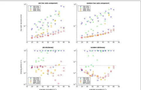
Figure 2 shows the recovery results for various cor-ruption levels using the corcor-ruption-adapted algorithms (ITKrMM) and their unadapted counterparts (ITKrM). We can see that for both representation pairs, incorpo-rating the corruption information into the learning algo-rithms clearly improves the performance. Another fact immediately visible is that for the adapted algorithms, the success rates differ for the two erasure modalities and decrease with increasing corruption level. However, the success rates do not depend much on the particular dis-tribution of the erasures or bursts as long as they lead to the same average corruption level. In contrast, the suc-cess rates of the unmodified algorithms depend very much on the corruption distribution, and signals with similar average corruption can lead to very different error rates.
We also observe that corruption can improve the recov-ery rates of both the unmodified and the modified algo-rithms. A similar phenomenon has already been observed for ITKrM in connection with noise and a lower sparsity level [29]. While one might expect the global recovery
rates to decrease with increasing noise and increasingS, they actually increase. The reason for this is that a lit-tle bit of noise or lower sparsity, like a litlit-tle bit of corruption, breaks symmetries and suppresses the fol-lowing phenomenon. Two atoms converge to the same generating atom, and therefore, another atom has to do the job (is a 1:1 linear combination) of two generat-ing atoms. For uncorrupted signals, there are ongogenerat-ing efforts to alleviate this phenomenon with replacement strategies, which will have a straightforward extension to corrupted signals.
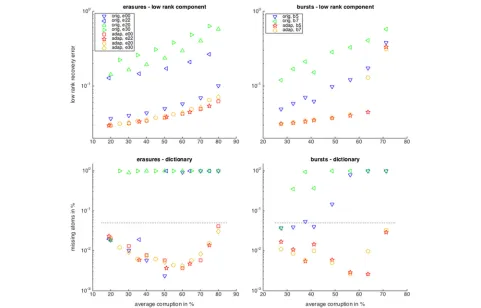
To find out when we gain most from incorporating the mask information, let us have a more detailed look at the recovery rates for different types of parameter set-tings. Among the random erasures, we distinguish 4 types. ‘type00’ indicates thatp1 = p2withp1varying between 0.2 and 0.8 andq1=q2=1, leading to a uniform erasure probability for all coordinates and all signals. ‘type20(30)’ indicate thatp2= p1+0.2(0.3)withp1varying between 0.1 and 0.7(0.6)and againqi=1, leading to higher erasure probabilities for the first half of the coordinates, which are however uniform across signals. Finally, ‘type22’ indicates thatp2=p1+0.2 andqi =piforp1varying between 0.4
and 0.8, leading to different erasure probabilities across coordinates and across signals.
Among the burst errors, we distinguish between ‘type5’ corresponding to a uniform burst distribution and ‘type7’ corresponding to a 0.7 probability of the burst occur-ring in the first half of the coordinates. For each type, we consider the burstlength T = 64 with probabili-ties(pT,p2T) ∈ {(0.5, 0.3),(0.7, 0.3),(0.5, 0.5)}leading to corruptions between 20 and 40% and the burstlength
T = 96 with the same pairs and additionally(p0,pT) ∈ {(0.3, 0.7),(0.1, 0.9)} leading to corruptions between 40 and 75%.
For conciseness, we focus on the random low-rank com-ponent and dictionary (Fig.3). Distinguishing between the different types, we can now see that incorporating the cor-ruption information gives the highest benefits when the corruption is most unevenly distributed over the signal coordinates. So, for the evenly distributed random era-sures and burst errors, ‘type00’ and ‘type5’, the low-rank component is still recovered by both the unadapted and the adapted algorithm, but as soon as there is interco-ordinate variance in the corruption level, type20/22/30’ and ‘type7’, the unadapted algorithm starts to lag behind. For the dictionary recovery, the unadapted algorithm
only does well for homogeneous corruption, ‘type00’ and ‘type5’, until about 50% corruptions but breaks down for higher corruption levels or for intercoordinate variance of the corruption, ‘type20/22/30’ and ‘type7’.
5.1.2 Spikiness and recoverability
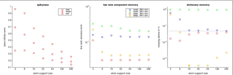
The second experiment explores the sensitivity of the adapted algorithms to the flatness/spikiness of the repre-sentation pairs, measured byγ∞ andφk∞. This is done by looking at the recovery of representation pairs, which form orthonormal bases and whose atoms have their energy concentrated on supports of sizemform=
4, 8, 16, 32, 64, 128, 256.
Dictionaries and low-rank components:For a given support size m, we choose d vectors zk from the unit sphere in Rm and d supports I
k = i1. . .im of size m uniformly at random and set B(Ik,k) = zk and zero else. We then calculate the closest orthonormal basis to
Busing the singular value decomposition. The first two elements of this orthonormal basis are chosen as the low-rank component, while the remaining elements form the dictionary.
Signals, corruptions and setup:For the signal genera-tion, we use the same parameters as in the last experiment,
and for the corruption, we use the random erasure masks of ‘type22’ withp1=q1=0.5/0.7 andp2=q2=0.7/0.9 corresponding to 36 and 64% of corruption. The experi-mental setup for the recovery of each representation pair is again as in the previous experiment. Figure4shows the spikiness of the representation pairs for various support sizes as well as the corresponding recovery results for the two corruption types. Let us first point out that our con-struction based on decreasing atom support sizes indeed leads to representation pairs with increased spikiness. As usual, the recovery errors incurred by the modified algo-rithms are much lower than those of the unmodified ones. For the low-rank component, the recovery error is very stable and only starts to deteriorate for m = 4, when the low-rank atom carrying less energy is indeed almost a spike,γ2∞ = 0.8997, meaning 80% of its energy are concentrated on one coordinate. Also, for the dictionary recovery, the robustness to spikiness of the adapted algo-rithms is quite surprising. So, for the low corruption level (36%), we always recover more than 95% of the dictionary atoms, and for the higher corruption level (64%), recov-ery only fails form = 4. As in the previous experiment, we observe the effect that spikiness like corruption can lead to better global recovery rates. The effect is more pro-nounced for the higher corruption level (64%), where for
m=16, we even have 100% recovery.
Before turning to experiments on image data, let us mention that we also briefly investigated the effect of the signal scaling on the recovery rates of the modi-fied algorithms for the DCT representation pair and the ‘type22’ erasure mask with 36% corruption, with the same setup as in the first experiment, but found that there was no strong influence. That is, forsmvarying between 2 and 128, the low-rank recovery error varies between 0.031 and 0.036 and the atom recovery rates stay between 95 and 96%.
Similarly, exploring the effect of the sparsity level S, we do not gain much more insights over the exper-iments already conducted in the uncorrupted case [29]. So, fixing all mask and signal parameters except for the sparsity parameter S, which increases from 4 to 16, the low-rank recovery error stays con-stant while the number of recovered dictionary atoms increases.
In order not to overload the paper, we do not detail these experiments here but refer the interested reader to the ITKrMM MATLAB toolbox1, which can be used to reproduce all the presented experiments and many more. 5.2 Numerical simulations on image data
In this section, we will learn dictionaries on image data, more precisely on image patches, and compare the learned dictionaries to those learned by wKSVD and BPFA as well as to analytic dictionaries. The first subsection consists of a comparison of the learned dictionaries and low-rank components in terms of coherence, supremum norm, sparse approximation qualities and the computational cost of the algorithms, while in the second subsection, we will use them for inpainting, meaning the reconstruction of the missing part in an image.
5.2.1 Dictionaries for image data
In the first experiment, we compare the ITKrMM dictio-naries to those learned with wKSVD and BPFA. Weighted KSVD [30,31] is an adaption of the original KSVD algo-rithm [9], intended to refine a prelearned dictionary based on available corrupted data that can be then used for inpainting, which we will discuss in more details in the next subsection. Similarly, BPFA [32], which is a nonpara-metric Bayesian method, can be used to learn dictionaries both from corrupted and uncorrupted data, where in the case of corrupted data, the dictionary is used for inpainting.
Data:For our experiments, we consider the grayscale imagesBarbaraandPeppersof size 256×256, which we corrupt by erasing each pixel independently with proba-bility 0.3 or 0.5 resulting in 30 resp. 50% erased pixels on average. We then extract all available 8×8 patches from the corrupted image as well as the corresponding mask and give the vectorised corrupted patch/mask pairs to the learning algorithms.
Algorithmic setup: Via ITKrMM, we first learn the low-rank component of sizeL=1, 3, 7, and a dictionary of sizeK=2d−L, resulting in a system with redundancy 2. We set the sparsity level in the dictionary learning to
S = 8−LforL= 1, 3 corresponding to an overall spar-sityL+S = 8 and toS = 5 forL =7, corresponding to an overall sparsityL+S = 12. For wKSVD, we use the setup corresponding to ITKrMM withL = 1 and learn a dictionary of sizeK = 2dwith the option of keeping the first atom always equal to the constant atomφ1 ≡ c. Since within wKSVD the contribution of the constant low-rank atom counts in the sparse approximation step, we use input sparsity levelS = 8. We use the same initialisation strategies as for the synthetic experiments, i.e. random vectors that are orthogonal to the low-rank component resp. low-rank atoms that have already been learned. This means that before subtracting the low-rank component, the initial dictionaries for ITKrMM and wKSVD are the same. For learning a low-rank atom, we use 10 itera-tions on all available patch/mask pairs, whereas for the dictionary learning step, we use 40 iterations on all avail-able patch/mask pairs for both algorithms. For BPFA, we use the out-of-the-box version provided on the authors’ website to learn 128 atoms from corrupted data using 150 iterations either with the recommended initialisation based on SVD or a random one. Since BPFA is a Bayesian
method, it has the advantage that no sparsity level has to be defined. Note also that the SVD initialisation makes sense in this context since due to the patch structure, the corruption is evenly spread over all patch coordinates.
Comparison:For comparison, we also learn dictionar-ies on the uncorrupted images. For KSVD with L = 1 and BPFA, we use the same setup as described above. For KSVD withL > 1 and ITKrM, we use a similar setup as in the synthetic experiments. This means that we choose as low-rank component the firstLprincipal components (left singular vectors of the data matrix), project all train-ing signals on the orthogonal complement of the low-rank component and then learn a dictionary of sizeK=2d−L
with sparsity levelS = 5 forL=3, 7 as well asS = 7 for
L=1 for ITKrM, on the projected signals.
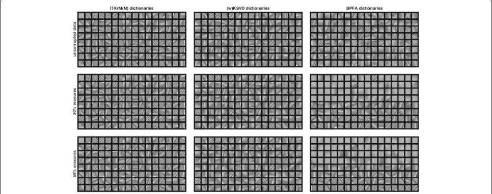
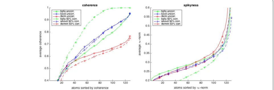
Consistency:Figures5and6show the dictionaries and if applicable low-rank components forL = 1 learned by ITKrM(M), (w)KSVD and BPFA with SVD initialisation from uncorrupted and corrupted data. The first impres-sion is that on uncorrupted data, the three algorithms produce quite similar dictionaries, even though ITKrM produces more high-frequency atoms than KSVD and the first BPFA atoms clearly have the structure of the principle components used in the initialisation. The next obser-vation is that ITKrMM and wKSVD are consistent, in the sense that most of the atoms learned on corrupted data have a corresponding atom in the dictionary learned on uncorrupted data. This is not true for BPFA, where the dictionaries learned from uncorrupted and corrupted data are markedly different, the latter containing many copies of the constant atom or slight variations thereof. This is naturally reflected in the coherence and spiki-ness of the dictionaries. Figure7shows the coherence of the dictionary atoms μk = maxj=k|
ψk,ψj
| and their
Fig. 6Dictionaries and low-rank atom (left upper corner) learned with ITKrM(M) (left), (w)KSVD (middle) and BPFA (right) algorithms on all 8×8 patches ofPepperswithout corruption (top), 30% erasures (middle) and 50% erasures (bottom)
supremum normψk∞sorted and averaged over five dif-ferent random mask realisation/initialisations for 0 and 50% corruption. ITKrM(M) produces the most incoherent and spikiest dictionaries, while BPFA produces the flattest dictionaries and on corrupted data also the most coher-ent ones. The reason for this might be that BPFA was not designed for consistency, but primarily for image pro-cessing tasks, such as inpainting, where flatness can be of advantage.
Approximation quality and low-rank components:
To illustrate the importance of integrating low-rank com-ponents into dictionary learning on real data, we test how sparsely the various representation systems learned on
Barbara approximate all image patches of Barbara. For every dictionary—low-rank—component pair, containing 128 atoms, learned either on clean or corrupted data, we
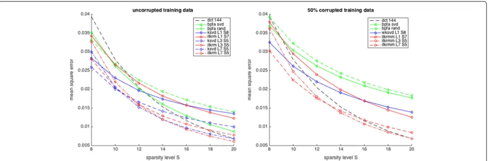
calculate the mean square error achieved by approximat-ing all clean patches, usapproximat-ing orthogonal matchapproximat-ing pursuit (OMP) and different sparsity levels from 8 to 20. Figure8 shows the results averaged over five different initialisa-tions and corruption patterns where applicable. Our first observation is that the dictionaries learned by KSVD and ITKrM on clean data with S = 5 and after removing a low-rank component of size L = 3 or L = 7 per-form best, indicating the importance of removing the low-rank component to get a well-conditioned dictionary. Similarly, the BPFA dictionary with SVD initialisation per-forms much better than the randomly initialised one. We also see that the advantage of the learned dictionaries over the overcomplete DCT for small S gradually decreases and vanishes at S = 20. Comparing to the dictionar-ies learned from corrupted data, we see that the wKSVD
Fig. 8Approximation quality of dictionaries with low-rank components of various sizes onBarbara, DCT144 as well as BPFA, (w)KSVD and ITKrM(M) learned on uncorrupted data (left) and on 50% corrupted data (right)
and ITKrMM dictionaries perform almost equally to their counterparts KSVD and ITKrM, the ITKrMM dictionar-ies giving the best performance, as the algorithm can also handle low-rank components withL>1. In contrast, the performance of the BPFA dictionaries degrades quite a lot, regardless of the initialisation. This is to be expected as the many copies of the flat atom, we have seen in Figs.5and6, essentially reduce the size and with it the approximation power of the dictionary.
Computation time:As both ITKrMM and wKSVD
pro-duce consistent and incoherent dictionaries with good approximation properties also from corrupted data, which is the main interest of this paper, we further compare them with respect to computational cost and memory require-ments. The cost per training signal of one iteration of ITKrMM consists of the inner product between the dic-tionary and signal,O(dK), the pseudo-inverse of ad×S
matrix together with some matrix vector multiplications for calculating the residual,OS2d+Sd, and the update ofS atoms based on the residual resp.S weight vectors based on the mask,O(Sd). All in all forNtraining signals, this amounts to a computational cost ofOdKN+S2dN
operations per iteration.
On the other hand, the cost per iteration of wKSVD consists of sparsely approximatingNsignals with masked OMP (see Algorithm 4) and the dictionary update. The cost of OMP per signal is lower bounded by the cost of the inner products between K atoms and the resid-ual forSiterations,O(SdK), which dominates the cost of the residual updates, OS2d+Sd. The update of each atom involves the calculation of the largest left singu-lar value of a matrixYk of approximate sized× SNK for several iterations. Using in turn an iterative procedure for the singular vector, we can lower bound the cost of one atom update by calculating the matrix vector prod-ucts Yk
Ykv, O(dSN/K). Thus, for N training signals,
the cost per iteration of wKSVD can be lower bounded byO(SdKN), meaning that ITKrMM is at least by a fac-tor min{S,K/S}cheaper. Note also that contrary to KSVD, the weighted version cannot be accelerated using batch OMP [34], as every mask changes the geometry of the dictionary. Both algorithms could be further optimised noting that a masked signal is projected ontomn= Mn2F coordinates. This means that all sparse approximation procedures could be done inRmninstead ofRd, and so
set-tingm= N1 mn, the cost estimate for ITKrMM reduces toOmKN+S2mNand for wKSVD toO(SmKN). In our implementations, we refrain from this option, since we doubt that in MATLAB, the multiplications by zero in full space are costlier than locating and accessing the correct coordinates.
Further comparing the memory requirements of the two algorithms, we see that ITKrMM needs about twice the size of the dictionary matrix O(dK). The memory requirements for wKSVD are much larger and corre-spond to the entire matrix of training signals,O(dN)or
O(mN), since the iteratively weighted dictionary update repeatedly accesses residuals, coefficients and masks. This also means that wKSVD cannot be used sequentially like ITKrMM.
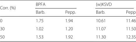
Table 3Speed-up of ITKrM(M) over (w)KSVD and BPFA,
corresponding to the average runtime of wKSVD/BPFA divided to that of ITKrMM using all available (corrupted) image patches of Barbara and Peppers
Corr. (%) BPFA (w)KSVD
Barb. Pepp. Barb. Pepp.
0 1.75 1.94 10.61 11.46
30 1.02 1.20 11.07 11.50
50 1.53 1.92 11.30 12.35
comparison to BPFA. We see that both on uncorrupted and corrupted data, ITKrMM is about 11 times faster than wKSVD, i.e. wKSVD takes about 3.5 h, while ITKrMM takes only about 18 min to learn a dictionary.
5.2.2 Inpainting
To demonstrate the practical value of the ITKrMM algo-rithm, we here conduct an image inpainting experiment. Inpainting is the process of filling in missing information or holes in damaged signals, and our motivating task, the prediction of blood glucose levels, can be cast as inpaint-ing problem. Image inpaintinpaint-ing, in particular, is used for restoration of old analogue paintings, denoising of digi-tal photos, and for removal of objects like text or date stamps from images and has become an active field of research in the mathematical and engineering commu-nities, with a variety of specifically developed methods and approaches [35]. Most of the existing approaches for inpainting are based on either variational approaches pioneered by Sapiro [36] or exploit image statistical and self-similarity priors as introduced by Efros [37]. With the advent of sparse representations and compressed sens-ing, sparsity-based inpainting has gained popularity in the recent years.
Since the primary goal of this paper is to evaluate the ITKrMM algorithm as a consistent and computationally efficient method for dictionary learning from incom-plete data, we perform a thorough comparison of the ITKrMM-based inpainting algorithm with other sparsity-based inpainting methods. In particular, we compare to the inpainting schemes based on wKSVD and BPFA dic-tionaries as well as analytic dicdic-tionaries such as the DCT basis and the overcomplete DCT frame with 144 atoms. In all cases, we show that our results are mostly better than the ones of BPFA and wKSVD, with a large reduc-tion of the computareduc-tional costs with respect to the latter. We also show that ITKrMM-based inpainting leads to bet-ter results compared to the ones obtained with the DCT dictionaries or more advanced methods, also based on analytic dictionaries, such as morphological component analysis (MCA)[6]. Last, we briefly compare our results to PLE [38], a state-of-the-art inpainting method for natural
images. PLE is based both on structured sparsity and sta-tistical priors on the sparse coefficient distribution and is known to outperform all simple sparsity based schemes.
Sparsity-based inpainting: Sparsity-based inpainting relies on the concept that the signalyisS-sparse in a dic-tionary, and therefore, the damaged signalMyis sparse in the damaged dictionaryM, that is for|I| ≤S
y≈IxI ⇒ My≈MIxI. (5)
To reconstruct the original signal one therefore simply needs to recover coefficientsx˜I ≈ xI by sparsely approx-imatingMyinMand to sety˜ = x˜I. However, for the sparse approximation of Myto recover the correct sup-portI, we do not only need that the signal is very sparse
S d but also that damaged dictionary Mremains incoherent, which translates to the original atoms hav-ing small supremum norm,φ∞ 1. In summary, the sparser the representation provided and the flatter the atoms, the better the dictionary is suited for inpainting. This means that BPFA dictionaries, which have very flat atoms, as discussed in Section5.2.1, might be better suited for inpainting than the wKSVD or ITKrMM dictionaries, which have comparatively spiky atoms, despite the fact that the latter provide sparser representations.
For sparse approximation of the coefficients, we use a slightly modified version of the well-known greedy algo-rithm, OMP [39, 40], which takes into account masked data. In particular, as the damaged dictionary is not nor-malised, we need to account for this in the OMP selection step and rescale by 1/Mφk2, similar to thresholding in the ITKrMM algorithm. Without this renormalisation, less damaged atoms take precedence over better fitting ones. The algorithm to which we refer as mOMP is described in Algorithm 4.
Algorithm 4 (Masked OMP for Inpainting (mOMP))
Given a damaged signal My together with the mask M, a dictionaryand a sparsity level S, initialise r=My, I= ∅ and while|I|<S andr2>10−3do
• Atom selection: find
j=arg max Mφk=0
| r,Mφk | Mφk2. • Approximation: Set
I=I∪{j},xI =(MI)†Myandr=My−MIxI.
Outputy˜=IxI.
Images: We consider six grayscale images, Barbara,
Peppers,House,Cameraman,MandrillandPirate, of size 256×256. The images are corrupted by erasing each pixel iid with probability 0.3, 0.5 or 0.7, resulting in 30, 50 or 70% erased pixels on average.
Learning setup: The dictionary learning setup is the same as in the experiments for 30 and 50% corruption levels in Section5.2.1, where for ITKrMM, we consider low-rank components of sizeL = 1 andL = 3, abbre-viated as ITKrMM1 and ITKrMM3 respectively. For 70% corruption, we reduce the sparsity level of ITKrMM and wKSVD in the learning stage to S = 3 and S = 4, respectively, and use onlyL = 1. This reduction is nec-essary because sparse approximation becomes difficult if the dictionary is coherentμ 1/S. In effective dimen-sion (average number of uncorrupted pixels per signal) 64·0.3 ≈ 19, a perfectly incoherent dictionary with 128 atoms already has coherence of at least 0.19>1/8, due to the Welch boundμ ≥
K−d
d(K−1). A randomly erased dic-tionary adapted to the data will be even more coherent, which renders learning withS=7/8 risky.
Inpainting sparsity level: We perform sparsity-based inpainting using mOMP with sparsity levels 4:4:24 and dictionaries learned by ITKrMM and wKSVD, the DCT basis, as well as an overcomplete DCT frame with 144 atoms. For BPFA, we report the results of both the accom-panying inpainting procedure as provided in [32], as well as the mOMP-based scheme used for the other dictionar-ies, abbreviated as BPFAomp. In the case of 70% erasures, we also include results of sparsity-based inpainting with a slight twist to deal with spikiness of the atoms. In par-ticular, to prevent inpainting with unreliable, ill-preserved atoms, we modify the mOMP selection step, so form =
M2F, we find
The results in Tables4and5achieved with this mod-ification are marked with an asterisk (*), for example ITKrMM*. We further compare the methods to MCA [6] as it is based on sparsity in a dictionary made of two ana-lytical orthonormal bases, such as wavelets, curvelets and DCT, for instance. Specifically, after comparing the per-formance of different combinations of bases for MCA, we present only the best results achieved by the undecimated discrete wavelet transform and curvelets. This combina-tion has also been used by the authors for one of the inpainting examples in the original code.
The results of wKSVD are generated with our own implementation modified from the original KSVD algo-rithm, as there is no MATLAB version openly available, while those of BPFA and MCA are produced by the origi-nal software and the authors’ recommended settings.
Comparison/error:We measure the recovery success of the schemes by the peak signal-to-noise ratio (PSNR) and the similarity index (SSIM) between the original image Y and the recovered version Y˜. For two images
YandY˜ of sized1×d2, the PSNR in dB is defined as
The SSIM index is defined as (2μY˜μY+c1)(2σY Y˜ +c2) dard deviations, and cross-covariance for imagesY˜ andY. For the similarity index, we take the default settings forc1 andc2with maximal image value 1. The results are aver-aged over 5 runs, each with a different mask and in case of ITKrMM and wKSVD different initialisations, to account for the variability between different mask realisations. For all OMP-based schemes, we only report the values corre-sponding to the sparsity level that gives the best result on average over the 5 trials.
Table 4 provides the PSNR values generated by all algorithms on the considered images. Inpainting with the DCT dictionaries gives relatively good results, even though the data-learned dictionaries like BPFA, wKSVD and ITKrMM outperform the DCT dictionaries all but once, the exception being Barbara with 30% erasures, where the very flat DCT basis is quite well suited to capture the textures.
On all other images with 30% corruptions the ITKrMM dictionaries provide the best results. In case of 50 and 70% random erasures, the wKSVD and ITKrMM dic-tionaries tend to divide the best performance between themselves. In particular, for more textured images like
Table 4Comparison of the PSNR (in dB) for inpainting of images with various corruption levels based on analytic dictionaries, DCT, MCA, and dictionaries learned on all available corrupted image patches, BPFA, BPFAomp, wKSVD, and ITKrMM (modified inpainting is marked with a *)
Algorithm Bar. Cam. Hou. Man. Pepp. Pir.
30% corruption Noisy Im. 11.17 10.81 10.11 10.82 11.18 11.70
DCT64 37.49 32.66 41.89 30.60 39.12 35.40
DCT144 37.08 32.41 41.49 30.86 38.90 35.42
MCA 35.89 32.45 39.62 28.38 35.59 33.35
BPFA 34.76 32.08 39.76 29.58 37.92 34.38
BPFAomp 35.36 32.23 41.09 30.81 38.66 35.42
wKSVD 35.87 32.62 41.42 30.41 38.64 35.09
ITKrMM1 36.12 32.80 41.97 30.85 39.20 35.60
ITKrMM3 37.16 33.04 42.30 30.92 39.80 36.08
50% corruption Noisy Im. 8.95 8.59 7.88 8.60 8.96 9.47
DCT64 32.72 28.56 36.65 26.99 34.01 31.10
DCT144 32.46 28.46 36.40 27.25 33.93 31.17
MCA 32.50 28.99 36.54 25.34 32.35 29.86
BPFA 32.97 28.89 37.71 27.25 35.29 31.89
BPFAomp 32.98 28.87 37.88 27.29 35.41 32.18
wKSVD 33.23 29.55 38.21 27.79 35.41 32.12
ITKrMM1 33.28 29.44 37.75 27.96 35.31 32.14
ITKrMM3 33.82 29.48 38.04 27.97 35.30 32.26
70% corruption Noisy Im. 7.48 7.13 6.42 7.13 7.50 8.01
DCT64 28.21 24.86 31.49 24.29 29.05 27.21
DCT144 28.09 24.81 31.37 24.44 28.81 27.32
MCA 28.74 25.71 33.42 23.29 28.56 26.55
BPFA 29.40 25.74 33.56 24.93 31.43 28.77
BPFAomp 29.22 25.61 33.05 25.10 31.12 28.63
BPFAomp* 29.23 25.60 33.04 25.11 31.18 28.74
wKSVD 29.70 25.89 33.96 25.09 31.17 28.76
wKSVD* 29.74 26.02 34.09 25.09 31.32 28.84
ITKrMM1 29.48 25.84 33.26 25.11 29.64 28.53
ITKrMM1* 29.93 26.34 33.65 25.12 31.26 28.83
The results are averaged over 5 random masks and initialisations. The best result for each setting is marked in bold
generic sparsity-based scheme using ITKrMM or wKSVD by about 1dB onHousewith 50 or 70% corruption and by about 3 dB onBarbara50% or corruption 70%.
For a more comprehensive comparison, we also present the average SSIM values of the reconstructed images for the various schemes in Table 5. The SSIM results are in general consistent with the ones for PSNR. However, for the 30% corruption level, inpainting with the DCT basis/frame provides slightly better values, followed by ITKrMM. Moreover, one can observe that for 50% cor-ruption, the SSIM values for the ITKrMM algorithms are slightly better than for all other algorithms—for 70% cor-ruption, they are better 4 out of 6 times. Compared to
the PSNR results for the same level of corruption, this essentially supports our previous conclusions that the tendency of ITKrMM algorithm towards high-frequency atoms allows to recover fine details, without too much oversmoothing. In contrast, the wKSVD algorithm, which sometimes has better PSNR values but worse SSIM values, leads to smoother images.
Table 5Comparison of the SSIM value (0.−) for inpainting of images with various corruption levels based on analytic dictionaries, DCT and MCA, and dictionaries learned on all available corrupted image patches, BPFA, BPFAomp, wKSVD and ITKrMM (modified inpainting is marked with a *)
Algorithm Bar. Cam. Hou. Man. Pepp. Pir.
30% Corr. Noisy Im. 1689 2367 0831 1604 1630 1619
DCT64 9822 9638 9813 9373 9859 9691
DCT144 9812 9629 9814 9413 9858 9698
MCA 9695 9500 9658 9218 9654 9552
BPFA 9438 9388 9608 8855 9710 9452
BPFAomp 9590 9564 9771 9400 9820 9688
wKSVD 9659 9551 9772 9341 9812 9662
ITKrMM1 9719 9597 9819 9418 9840 9701
ITKrMM3 9798 9612 9823 9428 9852 9729
50% Corr. Noisy Im. 1002 1617 0478 0899 1015 0946
DCT64 9503 9207 9542 8469 9647 9215
DCT144 9486 9194 9548 8566 9645 9239
MCA 9424 9173 9484 8408 9511 9157
BPFA 9284 9141 9508 8187 9612 9171
BPFAomp 9384 9222 9607 8782 9686 9377
wKSVD 9439 9257 9607 8786 9683 9363
ITKrMM1 9514 9281 9651 8816 9688 9374
ITKrMM3 9588 9281 9657 8825 9695 9392
70% Corr. Noisy Im. 0552 0981 0268 0459 0575 0515
DCT64 8703 8411 8976 6950 9115 8224
DCT144 8682 8389 8982 7081 9098 8275
MCA 8807 8592 9070 7056 9152 8363
BPFA 8783 8587 9231 7104 9366 8604
BPFAomp 8828 8600 9235 7614 9374 8713
BPFAomp* 8834 8602 9238 7615 9387 8740
wKSVD 8877 8648 9286 7616 9380 8750
wKSVD* 8885 8676 9290 7615 9392 8757
ITKrMM1 8937 8661 9306 7582 9222 8720
ITKrMM1* 9002 8749 9323 7583 9404 8753
The results are averaged over 5 random masks and initialisations. The best result for each setting is marked in bold
instance, manifests itself in the slightly better recovery of the texture on the trousers.
6 Discussion and conclusions
Inspired by real-life problems and applications, where data is incomplete and corrupted, we here extended the iterative thresholding and K residual means (ITKrM) algorithm for dictionary learning to learning dictionaries from incomplete/masked data (ITKrMM). To account for the presence of a low-rank component in the data, we fur-ther introduced a modified version of the ITKrMM algo-rithm to recover the low-rank component and adapted the ITKrMM algorithm to the potential presence of such