R E S E A R C H
Open Access
Dynamic time slot allocation and stream
control for MIMO STDMA in ad hoc networks
Wenwei Yue
1, Changle Li
2,1,3*, Yueyang Song
1and Lei Xiong
3Abstract
Multiple-input multiple-output (MIMO) technologies have been shown to potentially improve the performance of network. Many traditional medium access control (MAC) protocols, such as spatial time division multiple access (STDMA), may not support MIMO technologies directly and not make full use of the feature of MIMO, which may be a limitation in the practical application in ad hoc networks. Therefore, in this paper, we propose a dynamic time slot allocation and stream control for MIMO STDMA (DTSMS) protocol to improve STDMA in performance. Utilizing stream control technology of MIMO and reservation scheme, DTSMS makes improvement on network throughput and avoids the mutual interference of neighbor links. Thus, DTSMS can support both unicast and multicast simultaneously. Moreover, we implement the dynamic time slot allocation scheme in DTSMS to guarantee the transmission efficiency of packets with high cross-layer transmission parameters, such as the packet priority, neighbor node density, or link quality. Utilizing the collected cross-layer information, the proposed scheme allocates time slots for all nodes dynamically according to the changes of network topology and nodes’ transmission parameters. Finally, the effectiveness of the protocol is demonstrated by numerical analysis and simulations. The results show that DTSMS outperforms STDMA in terms of network throughput and delay. Furthermore, compared to our previous TTS-MIMO, DTSMS can decrease the delay of packets with high transmission parameters and improve the quality of service (QoS).
Keywords: Ad hoc networks, MIMO, STDMA, Stream control, Dynamic time slot allocation
1 Introduction
Ad hoc networks are an infrastructureless networks where nodes are often inexpensive off-the-shelf equipment with wireless transceivers, which could be organized anywhere at any time [1, 2]. Ad hoc technology is widely used and has become the key technology in many fields, such as social and biological networks. Many networks suc-ceeded in the recent years due to the development of ad hoc wireless technology [3], which obtains more and more attention. Nowadays, most of the medium access control (MAC) protocols in ad hoc networks are based on carrier-sense multiple access with collision avoidance (CSMA/CA) technology, but when the node’s quantity in a network is great and the network traffic is heavy,
*Correspondence: [email protected]
1State Key Laboratory of Integrated Services Networks, Xidian University, 710071 Xi’an, China
2State Key Laboratory of Rail Transit Engineering Informatization (FSDI), 710043 Xi’an, China
Full list of author information is available at the end of the article
CSMA/CA protocol, as a competitive multiple access pro-tocol, cannot satisfy the quality of service (QoS) require-ments well. We are considering utilizing time division multiple access (TDMA) mechanism to reduce collisions and improve network throughput.
In general, MIMO technologies, which refer to using multiple related or unrelated antennas to send or receive data, make full use of the space dimension of communica-tion system, broaden the applicacommunica-tion of tradicommunica-tional quan-titative Shannon, and provide a new method to utilize the antenna arrays. MIMO technologies at the physical layer have been widely studied and applied in ad hoc networks; however, the advantages of MIMO, such as flexibility and network throughput improvement, could be uti-lized effectively only by designing appropriate upper-layer protocols. Moreover, with the advent of 5G technology [4, 5], the effective upper-layer protocols are significant to increase the capacity, reduce latency, and improve the energy efficiency of current mobile networks [6]. There-fore, to design better MAC protocols supporting MIMO
for ad hoc networks is essential for the rapid develop-ment of MIMO technologies. There are many classes of MIMO MAC protocols, such as stream control-based [7], encoding-based [8], and beamforming-based [9]. We mainly focus on MIMO MAC protocols based on TDMA in this paper.
Traditional TDMA MAC protocols cannot fully mul-tiplex channels, so spatial time division multiple access (STDMA) protocol in [10] is proposed to make full use of the channel of the network. STDMA is the exten-sion of TDMA, which enables long-distance mobile nodes to share the same time slot to improve the throughput of network. In STDMA, space is divided into several virtual space slots and there are many nodes in each vir-tual space slot. If the distances between nodes are large enough, these nodes can transmit data in the same time without collision. In this way, STDMA can implement spatial reuse and increase network capacity. There have been many researches on the STDMA protocols in ad hoc networks [11, 12]. However, these protocols utilize the single-input single-output (SISO) technology. In addi-tion, most of the MIMO MAC protocols are used for either unicast or multicast instead of supporting both simultaneously, which could be a limitation in practical applications.
Over the past years, a variety of aspects of MIMO MAC protocols in ad hoc networks have been studied. The authors in [7] propose centralized and distributed stream-controlled medium access (SCMA) protocols in order to maximize network resource utilization and ensure the fairness of network. However, SCMA proto-col costs much to obtain the whole network topology, and furthermore, nodes’ mobility reduces its efficiency. The authors in [13] try to use spatial multiplexing and beam-forming technologies to improve network capac-ity. In [14], the authors propose a spatial diversity MAC (SD-MAC), which uses space-time block codes to obtain diversity gain and reduce the effect of channel fading. The authors in [15] propose a mitigating interference using multiple antennas (MIMA) protocol which uses a cross-layer design between MAC layer and physical layer [16] to reduce interference and improve network throughput. However, every transmission just uses half antennas in MIMA, which is a limitation that MIMA cannot adjust antenna numbers according to different scenarios.
The study of MIMO MAC taking into account TDMA is pioneered by [17, 18]. The authors in [17] use MIMO-OFDM technology and space-time block codes to achieve parallel transmission, but busy tone channel cost addi-tional overhead. The protocol in [18] allocates each node time sub-slots to reserve and raises time slot uti-lization using MIMO technology. Moreover, cross-layer MAC design [15, 19, 20] is also used to improve the
performance of networks. To break the strict limita-tion of the communicalimita-tion between layers, cross-layer MAC design fully considers the relationship of each layer and allows exchanging information between layers on the basis of the original protocol stacks [21]. In terms of dynamic resource allocation, there are many existing methodologies to allocate the network resources (e.g., bandwidth [22], power per subcarrier [23], time slot and subchannel [24]) for nodes in the networks, which enhance the QoS and guarantee the packet transmission efficiently. Therefore, on the one hand, we can use the cross-layer information to adjust the transmission strat-egy adaptively to satisfy requirements of high layer, and on the other hand, we can also utilize them to implement time slot allocation for all the nodes in ad hoc networks. However, most of the existing time slot allocation schemes in ad hoc networks do not take the cross-layer informa-tion and the changes of network topologies [25, 26], which have the poor adaptability to network topology changes and cannot guarantee the QoS of the packets with high cross-layer transmission parameters.
Therefore, the main problem we address and the cor-responding contribution of this paper is implementing a multiple access protocol in ad hoc network based on STDMA supporting MIMO, which can be divided into the following aspects specifically:
• Because most of MIMO MAC protocols are utilized
for either unicast or multicast, in this paper, we propose a new MIMO STDMA (DTSMS) protocol using a stream control scheme. We implement three kinds of CTS packets to control the number of data streams to send data aimed at different cases; in this way, DTSMS protocol can support unicast and multicast simultaneously and improve the performance of the STDMA protocol.
• We implement dynamic time slot allocation scheme
in DTSMS protocol to adjust the transmission time slots for all nodes according to the changes of network topologies and cross-layer information. Thus, DTSMS can decrease transmission delay of packets with high cross-layer transmission parameters (e.g., the video information in the city center) and improve the QoS further.
2 System model
2.1 MIMO model
Senders and receivers are equipped with multiple anten-nas in MIMO system, which can obtain diversity gain, multiplexing gain, and interference suppression ability to improve transmission performance. MIMO antennas are usually modeled by spatial degree of freedom (DOF). For a node withMantennas, it is generally considered to own
MDOFs. For a MIMO link, its spatial degree of freedom is defined as the smaller DOF of the node on both sides of the link. For instance, the degree of freedom for the link, in which the DOF of sender isMsand the DOF of receiver is
Mr, ismin(Ms,Mr). In the case of no interference streams, the link owningmin(Ms,Mr)DOFs can transmit at most
min(Ms,Mr)data streams. If interference streams existed, a part of DOF owned to receiver is used to suppress inter-ference streams [7], so the number of data streams that the link can transmit will be less thanmin(Ms,Mr). In general, suppressing interference streams is done by the receiver. For example, a node ownsMrDOFs can receive
Ksdata streams and suppressKjinterference streams suc-cessfully if they satisfyKs + Kj ≤ Mr. Without loss of generality, nodei can receive all data streams, if the sum of data streams and interference streams sending to node i is not greater than the DOF of node i, that is
s
Ks +
j
Kj ≤ Mi.
MIMO can provide stream control gain for MAC layer protocols. Assuming that each node ownsMDOFs, each link also ownsMDOFs. If there areminterfering links, maximum data streams transmitted on each link are
K = M/m(M/mmeans the integer part ofM/m), which is available to be employed to suppress interference streams. The gain achieved through such stream control is termed as stream control gain. In STDMA mode, for example, two links are arranged in different time slots, and each link usesMdata streams (e.g., each stream is
25 kbps) for transmission. However, in stream control mode, these two links choose the best two streams (e.g., each stream is 30 kbps) to transmit in the same time slot, which provides an improvement about 20% in network capacity (120 kbps), compared to that in the TDMA mode (100 kbps). It has been proved that performing stream control mode could obtain up to 65% improvement in performance over the STDMA mode when measured at indoor channels in the presence of low correlation.
2.2 Network model
We assume that an ad hoc network consists ofN nodes, where each node can be denoted asi ∈ N. Node ihas interference with nodejif the signal-to-noise ratio (SNR) on the link from node i to node j is greater than or equal to a certain threshold [27], which is expressed by formula (1),
SNR(i,j)= Pi
Lb(i,j)Nr ≥γ0
, (1)
in which Pi indicates the transmission power of node i, and the path loss of this power to nodej is denoted as
Lb(i,j). Nr indicates the effect of the thermal noise. If the link from nodei to nodejsatisfied (1), we say that nodei andjare in the same contention area. As nodes in the network are distributed sparsely, several separated contention areas may exist according to the space.
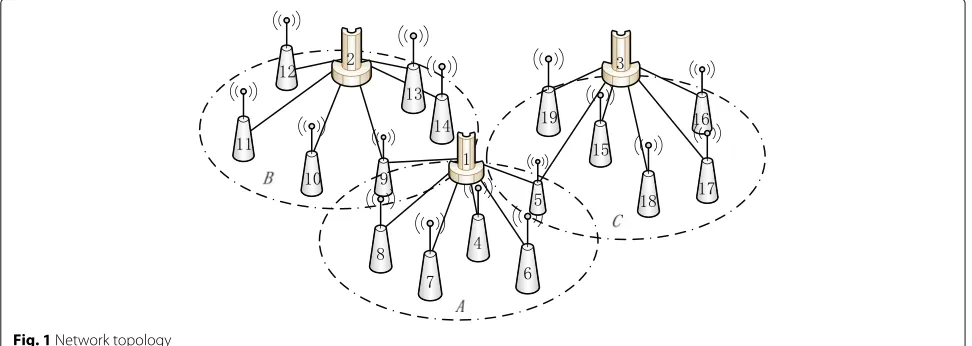
A network topology of 19 nodes is shown in Fig. 1, and areasA,B, andCare three contention areas. Contention area is defined as a special area where nodes cannot use the same time slot to send data, such as nodes 6, 7, and 8 in areaA. Nodes in different contention areas can be reused in the same time slot, such as nodes 7, 10, and 15, which belong to areasA,B, andC, separately. In each con-tention area, there is a center node which controls the time slot allocation in the contention area where it is allocated. In order to reduce the interference, the distance between
center nodes in different contention areas must reach to a certain value. In Fig. 1, nodes 1, 2, and 3 are center nodes and satisfy the condition above.
3 DTSMS protocol
The dynamic time slot allocation and stream control for MIMO STDMA (DTSMS) protocol is based on STDMA, which is a wireless MAC protocol for ad hoc networks, and it enables long-distance mobile nodes to share the same time slot for the purpose of improving network throughput.
The DTSMS protocol aims to utilize cross-layer infor-mation, such as traffic arrival rate, neighbor node density, and packet priority, to provide nodes with dynamic time slot allocation and support both unicast and multicast at the same time. The protocol could satisfy the QoS require-ment in terms of delay, and network throughput is also improved by exploiting MIMO technology.
In order to satisfy the QoS requirement, each node needs to send HELLO packets in each cycle to obtain neighbor node density. Here, a cycle is defined as the period that consists of allocated time slots of all nodes. Then, each node sends cross-layer information, includ-ing traffic arrival rate, neighbor node density, and packet priority to the center node, as a basis to decide time slot allocation. Therefore, time slot allocation is con-sidered about the service’s characteristics and is also adjusted periodically and dynamically according to the changes of network topologies and the cross-layer infor-mation. In this way, the higher the packet priority, the higher the neighbor node density, and the better the link quality a node has, the earlier the node sends data packets.
Besides that, nodes could use clear channel assessment (CCA) technology to occupy idle time slots and send pack-ets in order to avoid the waste of time slots. Network throughput is also improved with collision resolution by exploiting MIMO technology. The details of the protocol are described in the following subsections.
3.1 Stream control scheme
We consider node Sas a sending node and node Ras a receiving node; each node ownsMDOFs. For the purpose of taking full advantages of MIMO, stream control scheme is proposed. By using several types of CTS packets, we can choose the number of data streams to transmit data. CTS packets have three types which are used in three differ-ent cases, respectively. The three kinds of CTS packets are described as follows:
1. The CTS I packet is used when nodeRonly receives 1 RTS packet for itself without hearing any other RTS packets from other nodes at the same time. In this case, nodeRreplies to a CTSIpacket to nodeSto inform it to use all DOFs for this data transmission.
2. The CTS II packet is used when nodeRreceivesNRTS packets for itself without hearing any other RTS pack-ets from other nodes at the same time. In this case, nodeRreplies to CTS II packets to inform nodes who send RTS packets to nodeRthat they could useM/N
DOFs for this data transmission.
3. The CTS III packet is used when node R not only receivesN RTS packets for itself but also hears other RTS packets from other nodes at the same time. In this case, nodeRreplies to CTS III packets to inform nodes who send RTS packets to nodeRthat they could just use one DOF for this data transmission. RTS packets, CTS packets, or ACK packets are sent by only one DOF, which is good for avoiding collision.
3.2 Dynamic time slot allocation scheme
In order to shorten the average packet queuing delay fur-ther, we are going to consider neighbor node density and packet priority. After choosing proper time slot length, we make use of neighbor node density and packet priority to adjust time slot allocation to satisfy QoS requirement better.
In the DTSMS protocol, we choose neighbor node den-sity in the network layer, packet priority in the MAC layer, and link quality in physical layer as three factors which could decide the time slot allocation, since these three factors are related to the performance of unicast and multicast. The packets of higher priority need to be trans-mitted in a lower delay, and the packets of lower priority may not care about delay. Each node sends neighbor node density and packet priority to the center node, and then, the center node calculates theQiaccording to formula (2). According to theQi, the time slot allocated to a node is determined and changes with the topology of network.
Qi =piωpi+diωdi+liωli, (2)
where pi, di, andli are the priority, neighbor node den-sity, and link quality of theithnode, respectively.ωpi,ωdi,
andωli are the normalization coefficients of the priority,
neighbor node density, and link quality.
3.2.1 The cross-layer information weight determining mechanism
In order to get the expression of the transmission fac-tor, we need to calculate the normalization weight of the packet priority, neighbor node density, and link quality, respectively. In this way, we build the straight reciprocal matrix of weight by comparing the influence to data trans-mission of any two of the influence factors. Then, we use power method [28–30] to calculate the maximum eigen-value and its eigenvector of the matrix. After we normalize the eigenvector, we can getωpi,ωdi, andωli. The process
According to the impact of the cross-layer information to packet transmission, we can build a 3∗3 straight recip-rocal matrix, and every element in the matrix is the weight ratios of any two of the cross-layer information. Actually, the accurate weight ratios of the cross-layer information are hard to be estimated which can be chosen according to the actual requirements and users’ preference. There-fore, we take an example to indicate the build process of the straight reciprocal matrix which can be presented as formula (3),
priority, neighbor node density, and link quality, respec-tively.
Because matrix A is a positive reciprocal matrix whose maximum eigenvalue λmax is the simple multiplicity of eigenvalues. For the other eigenvaluesλ, they all follow:
λmax>|λ|. (4)
Given the eigenvalues of the N-order matrix are λ1,
λ2,. . . ,λn, where
|λ1|>|λ2|> . . . >|λn|. (5) And the relevant linearly independent eigenvectors are
u1,u2,. . .,un. Thus theneigenvectors can be a set basis
whereαipresents theithcoordinate under this basis. Then, we can use the iteration formula (7) to obtain the eigenvector.
x(k+1)=Ax(k) k=0, 1, ... (7)
Thus, we can get:
x(1)=Ax(0)=A
Therefore, we can get
lim
In this way, we can get the equation
lim
k→∞εk=0. (14)
And the speed of convergence depends on the ratior=
λ2 λ1
, and the smaller theris, the faster the convergence speed will be. Therefore, whenkis large enough, we can get
x(k)=λk1α1u1. (15)
On the one hand, if|λ1| > 1, whenkis large enough,
λk
1will be very large which cause some difficulties to the
calculation. On the other hand, if|λ1|<1, whenkis large
enough,λk1will be very close to 0 which is also a problem to the calculation. Therefore, we can follow the formula (16) by transforming the vector after each iteration into the vector whose maximum component is 1.
⎧ value of the absolute value of the maximum eigenvalue after thekthiteration andx(k + 1)is the relevant eigen-vector. We assignεas 0.001. Thus, as Table 1 shows, when
Table 1Iteration results
x(k) [1, 1, 1] [4.5, 2.8667, 2.333] [2.9926, 1.9259, 1.5494] [3.0008, 1.9315, 1.554] [3.0013, 1.9318, 1.5543]
|βk+1 − βk| < 0.001, we consider the maximum eigenvalue has met our requirements.
Finally, we normalize the eigenvectorx(k + 1), and the normalized eigenvector is
[ 0.4626, 0.2978, 0.2396] . (17)
Therefore, the expression of transmission factorQiis
Qi=0.4626pi+0.2978di+0.2396li. (18)
3.2.2 Dynamic slot allocation algorithm
Definition 1Equivalent nodes: Two nodes in the same contention area have the same connectivity with the other nodes. And if node i and node j are equivalent, which can be presented as
Take the network topology in Fig. 1 as an example; according to the definition, we can get three equivalent node groups [6, 7, 8], [13, 14], and [16, 17, 18]. Moreover, in order to make use of STDMA, all the nodes should be allocated into different time slots and the nodes in the same contention area should not be allocated in the same time slot.
Therefore, all the 19 nodes in the network can be divided into six time slots, and all the feasible schemes can form a setU. At first, we should choose one allocation scheme fromUto send data randomly. Then, if the network topol-ogy does not change, hub will record the transmission fac-torQof transmission nodes and adjust the transmission sequence among the equivalent node groups according to the transmission factorQ. The larger the transmission fac-torQof the transmission nodes are, the earlier the data in the nodes will be transmitted. However, if the network topology changes, the hub should calculate the average accumulated transmission factorE[Q] of all the time slots. The average accumulated transmission factorE[Qj] of the
jthtime slot can be presented as
E[Qj]=
where mj is the number of transmission nodes is the
jth time slot. Finally, the hub will calculate the scheme parameter K of all the allocation schemes inU accord-ing to formula (21) and choose the allocation scheme with the minimum scheme parameter K as the new time slot allocation scheme. The process is presented in Algorithms 1.
K=
6
j=1
jE[Qj] . (21)
Algorithm 1Dynamic time slot allocation algorithm 1: whiledata receive/transmission process is in process.
do
2: Choose a feasible time slot allocation scheme ran-domly from all the obtained allocation schemes.
3: Find the equivalent nodes groups in the network according to formula (19).
4: whilenetwork topology changesdo
5: Calculate the average transmission factor of each slot according to formula (20).
6: Calculate K of all the allocation schemes inU according to formula (21).
7: Find the allocation scheme with minimumK as the time slot allocation scheme.
8: end while
9: Record the transmission factorsQof all the trans-mission nodes.
10: Exchange the sequence among all the equivalent nodes groups according to the value of transmission factorsQ.
11: end while
3.3 Communication process description
Firstly, each node sends traffic arrival rate to the cen-ter node, which calculates tslot1 and tslot2 with the
QoS requirement.tslot1is the minimum time slot length
when slot utilization reaches maximum αmax, and tslot2
is the maximum time slot length when average packet queuing delay satisfies the QoS requirement approxi-mately. If tslot1 ≤ tslot2 as the later discussion shows,
we will choosetslot1as the time slot length; thus, slot
uti-lization is maximum and average packet queuing delay is lower. And if tslot1 > tslot2, we will choose tslot2
as the time slot length, because we choose to satisfy the QoS requirement about delay at the cost of slot utilization.
Then, in the time slot allocated to nodeS, if the traf-fic is unicast, the nodeSsends RTS packet directly, and if the traffic is multicast, the nodeSsends packet of mul-ticast directly using full antennas. In the idle time slot unallocated to node S, the node S reserves channel to realize unicast or sends data packet of multicast using one antenna. According to types of receiving CTS packet, node S selects appropriate number of streams to send data packets. When a data packet of unicast is received successfully, node R replies ACK packet to node S for confirmation. Otherwise, a failed transmission occurs and nodeSneeds to retransmit the data packet. ACK packet is unnecessary in multicast transaction. The operation pro-cess of nodeSand nodeRis shown in Algorithms 2 and 3, respectively.
We take the transmission case in the slot 1 of area A
as a specific instance to analyze operation procedure in DTSMS, and the operation procedure in other contention areas are similar as this instance.
If the node is in a contention area, such as node 7, the node can receive 1 RTS packets and send data using all the four antennas. However, if the node is in differ-ent contdiffer-ention areas, such as node 5, it can receive many RTS packets or multicast packets and utilize the corre-sponding CTS packets to control the number of data streams.
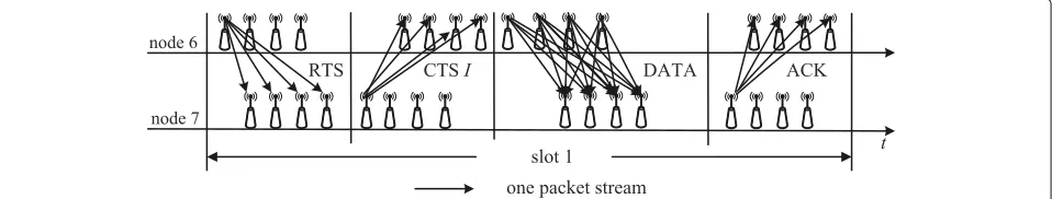
As shown in Fig. 2, when node 6 sends data packets in its own slot using unicast, node 6 can send RTS packet directly in the slot. Thus, node 7 can only receive one RTS and cannot hear any other RTS packets from other nodes in the same time slot. Node 7 replies CTS I packet to node 6 and indicates that node 6 can transmit data using four antennas. When node 7 receives data packets from node 6 successfully, node 7 replies ACK packet to node 6. Mean-while, other nodes will keep quiet in this time slot until the next time slot.
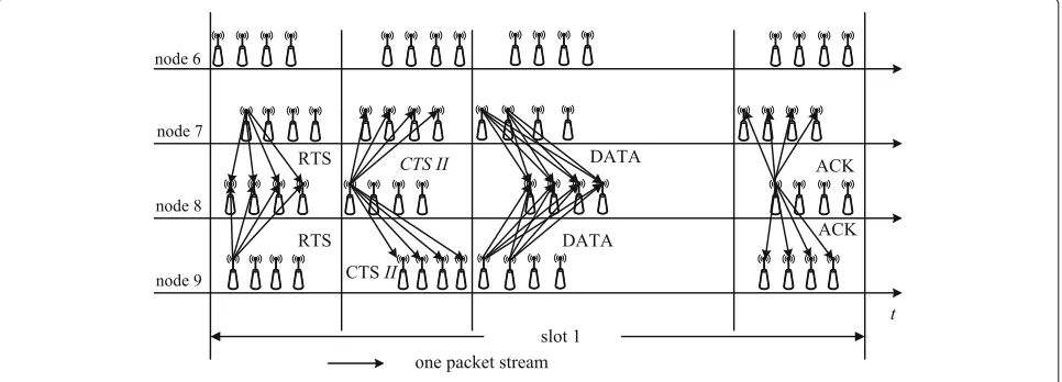
Figure 3 shows the scenario where node 6 has no data packet to send in its allocated time slot. However, node 7 and node 9 have data packets of unicast to send to node 8 in this slot. After they do CCA and find the channel is idle, they send RTS packets to make reservation. Thus, node 8 will receive 2 RTS packets and reply a CTS II packet to nodes 7 and 9 notifying them to send two parallel data
Algorithm 2Operation process of nodeS
1: whiledata receive/transmission process is in process.
do
2: Time slot is allocated by center nodes according to Qi.
3: whiletime slotndo
4: ifn= time slot allocated to nodeSthen 5: ifunicastthen
6: Send RTS to nodeRwithout CCA. 7: else
8: Send multicast packet usingMantennas.
9: end if
10: else
11: Do CCA.
12: ifchannel is idlethen
13: ifunicastthen
14: Send RTS to nodeRto reserve channel.
15: else
16: Send multicast packet using 1 antenna.
17: end if
18: else
19: Delay this transmission until next time slot.
20: end if
21: end if
22: Wait CTS packet. 23: ifCTSIthen
24: Send packets to nodeRusingMantennas. 25: else ifCTSIIthen
26: Send packets to nodeRusingM/N anten-nas.
27: else ifCTSIIIthen
28: Send packets to nodeRusing 1 antenna.
29: end if
30: n++. 31: end while
32: Record the transmission factor Q. 33: ifthe network topology changesthen
34: Time slot is allocated by center node according to Qi.
35: end if
36: end while
Algorithm 3Operation process of nodeR
1: if received RTS for itself and heard no other RTSs
then
2: ifRTS = 1then
3: Reply CTSIto nodeS. 4: else
5: Reply CTSIIto nodes who send RTSs to it. 6: end if
7: else ifheard multicast packetthen
8: Give up replying CTS to nodes who send RTS to it. 9: else
10: Reply CTSIIIto nodes who send RTSs to it. 11: end if
streams, respectively. In this way, the idle time slots can be utilized, but also, the process can make full use of the interference suppression in MIMO technologies to avoid collision efficiently.
Figure 4 shows the transmission procedure that the receiving node not only receives RTS packet for itself but also hears other packets for other nodes at the same time. If node 6 has no packet to send in its allocated slot and node 8 and node 4 have data packets to send to node 9 and node 5, respectively, then they will send RTS pack-ets to make reservation. However, in this case, node 9 will not only receive a RTS packet from node 8 but will also hear a RTS packet from node 4. Therefore, in order to avoid collision, node 9 and node 5 send CTS III packets to node 8 and node 4 to notify them to send one data stream, respectively.
3.4 Scenarios
We make some assumptions regarding the previous sub-sections of DTSMS:
1. The network topology is shown in Fig. 1, and each node has 4 DOFs in the network.
2. All the nodes keep moving in the network and the positions of node 1, node 2, and node 3 are almost unchanged relative to other nodes.
3. Nodes within one-hop range are
mutual-communicated, and nodes within two-hop range are mutual-sensed.
4. The node 1, node 2, and node 3 are center nodes in each contention area. The cross-layer information can be transmitted to the center nodes to calculate the transmission factors of transmission nodes according to formula (2).
5. According to the transmission factors of every node, the time slots are allocated dynamically.
4 Performance analysis
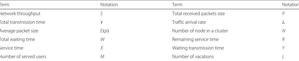
In this section, we analyze the throughput and delay of our proposed protocol under unsaturation condition. We take the nodes in area A as a specific instance to analyze the performance of the protocol because the operation procedure in other contention areas is similar as in this instance. Moreover, we consider every node is only in one contention area. That is to say, the nodes which are located in the different contention areas are ignored. Table 2 lists the important notation that is used in this paper.
4.1 Throughput
Suppose there are N nodes in the network and every node has at least M different packets to send simulta-neously by using all M DOFs at the start of its own slot. However, if some slots which have been allocated to nodes are idle, other nodes may occupy the idle slot to send packets. The number of antennas used to send packets depends on the kind of the RTS packet it receives.
Fig. 4Node receives RTS packet and heard other RTS packets
Let S be the network throughput, P be the total received packets size, andτbe the total transmission time, then
S= P
Nτ. (22)
According to the stream control model,Pconsists of two parts: the packet sizePin sent by the owner of this time slot andPoutby other nodes if the owner of this time slot has no packets to send.
For one thing, if the node has data packets to send in the allocated time slot, according to the operation process in the system model, it can use allMDOFs to send packets. LetPnbe the packet size of thenthpacket,λbe the traf-fic arrival rate, andNtbe the number of received packets; the total received packet sizePin using 1 antenna can be shown as
Pin= Nt
n=1
Pn. (23)
The mathematical expectation of total received packet size can be shown as
E[PNt]=E[E[PNt|Nt] ]
= ∞
k=1
E[PNt|Nt=k]p(Nt=k)
=E(P)
∞
k=1
k∗p(Nt=k)
=E(P)∗λτ,
(24)
whereE(P)presents the average packet size.
Moreover, the DOFs of the process isM, and the math-ematical expectation ofPinis
Pin=M∗E(P)∗λτ. (25)
For another, if the node has no packets to send in its allocated time slot, the number of antennas used to send packets is different in this process. LetNbe the number of nodes in a cluster,Vbe the number of requested anten-nas andpbep(Nt = 0). If there is only one node sending packets, in this case, according to the operation process,
Table 2Notation list
Term Notation Term Notation
Network throughput S Total received packets size P
Total transmission time τ Traffic arrival rate λ
Average packet size E(p) Number of node in a cluster N
Total waiting time W Remaining service time R
Service time X Waiting transmission time Y
this node will receive the CTS I packet and useM anten-nas to send packets. The probability of this case can be presented as
If the receiving node has receivekRTS packets for itself and not heard any other RTS packets from other nodes at the same time, in this case, it will reply a CTSIIpacket to theksending nodes and the sending nodes will send pack-ets usingM/kantennas. The probability of this case can be presented as
If the receiving node has not only received RTS packet for itself but also heard other packets for other nodes at the same time, in this case, it will reply a CTSIIIpacket to the sending node to notify it to send one data stream. The probability of this case can be presented as
p(V=1)
Therefore, the mathematical expectation of the number of antennasVcan be presented as
E(V)=M(N−1)e−λτ(N−2)(1−e−λτ)
Moreover, the mathematical expectation ofPinis
Pout=E(V)∗E(P)∗λτ. (30)
Above all, the throughput can be presented as
S= (Pin+Pout)(1 − p)p
We use the queue theory to analyze the delay of our DTSMS protocol. In this protocol, we use STDMA pro-tocol to allocate the time slots for every node in ad hoc networks; therefore, the nodes can send their packets in their allocated time slots and sleep in other time slots. In this way, we can use M/G/1 queues with generalized vacations to analyze the delay of this process.
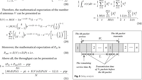
As shown in Fig. 5, suppose when theithpacket arrives, there areNi packets in the queue, and thelthpacket is receiving services and its remaining service time isRi. Let the service time of the kth packet be Xk and the wait-ing transmission time of other nodes beYi; therefore, the waiting time of theithpacket is
Wi=Ri+ i−1
k=i−Ni
Xk + Yi. (32)
Let the service rate beμand the proportion of packet transmissionρ = μλ; therefore, the expression of waiting timeW is
W= R + Y
1 − ρ. (33)
As Fig. 6 shows, the shaded parts are the remaining ser-vice timer(t)of packet transmission and the other parts are the remaining service time of vacations.
Suppose the M(t) andL(t) are the number of served users and vacations in the time periods [0,t], respectively, and the average remaining service time can be presented as
Fig. 6Model of remaining service time
where Mt(t) is the average packet arrival rate, L(tt) is
the average vacation arrival rate,
M(t) The periods of packet transmission and vacations are full of the whole time, so the proportion of packet trans-mission isρ and the vacation arrival rate is 1−Vρ where λis the packets arrival rate andμis the service rate. Let
t → ∞, and the average remaining service time can be presented as
However, if some nodes have no packets to be trans-mitted, the other nodes could occupy idle time slots and send packets. The remaining service time of this process is shown in Fig. 7. Suppose some nodes have no packets to be transmitted in vacationsV1 andV2 and the node transmitting packets in the first time slot occupies the idle time slots and sends packets. However, as shown in Fig. 7, although the node occupies the same number of time slots in vacationsV1 andV2, the remaining service time is different and the longer the continuous vacations are, the longer the remaining service time is. Moreover, the remaining service time is related to the number of time slots the node can occupy and the sequence of the occupied time slots.
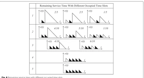
As we can see in Fig. 8, the first column in the figure means the number of occupied time slots and the sec-ond column illustrates the remaining service time with different occupied time slots and the probability of all the
Fig. 7Remaining service time in DTSMS
cases. It is important to note that every remaining service time diagram r(t) in the figure is just a typical example of each case and we do not list all the cases for simplic-ity. Moreover, the third column illustrates the value ofr(t)
corresponding to different number of occupied time slots whereτis the length of a time slot.
Therefore, according to the number of antennas used to transmit packets in Algorithm 2, the formula (35) can be presented as
whereRis the remaining service time during the period vacation time, V represents the average vacation time after the idle time slots occupation, andXrepresents the average transmission time during the primary vacation time.
Moreover, letVmandp(Vm)be the vacation time and the probability, respectively, of themthline in Fig. 8, so the vacation time of themthlineVm is
Vm =mτ. (37)
Similarly,V2
m can be presented as
V2
mnandp(mn)are the second moment of vacation time and the probability of thenthdiagram in themthline, respectively, which have been labeled in Fig. 8.
Then, the average transmission time during the primary vacation timeX2
mis
X2
m=(5−m)τ2. (39)
Above all, letrm be the remaining service time during the vacation time and we can get the expression ofrm
rm=
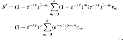
Therefore, the remaining service time during the period vacation timeRin formula (36) can be presented as
R=(1−e−λτ)5−m
Fig. 8Remaining service time with different occupied time slots
transmission time slot. However, if theithpacket belongs to the(l − 1)thnode, this packet needs to wait for five transmission time slots.
Therefore, suppose theithpacket of the(l+j) mod 6 node arrives in the transmission time slot of thelthnode, the waiting transmission timeYi = (j mod 6)∗τ when there are no idle time slots. However, if the transmission node occupies the idle time slots, the waiting transmis-sion time will be shortened. The average waiting trans-mission timeYis
Y= 1
6
5
m=1
Yi= 1 6
5
m=1
(1−e−λτ)m
m
j=0
(m−j)τ. (42)
Putting formula (36), formula (41), and formula (42) into formula (33), the average waiting time can be presented as
W= 1
1−ρ 1
2λX2
M +
R E(V) +Y
. (43)
5 Simulations
In order to verify the validity and effectiveness of DTSMS, in this section, we finish some simulations according to the protocol we propose above in MATLAB. Firstly, based on the network topology in Fig. 1 and the analysis results in Section 5, we compare the network throughput and delay of DTSMS with that of STDMA and TTS-MIMO [31]. Then, we compare the transmission factor Q and the cross-layer information of all the time slots under the same scenario to verify the effectiveness of the dynamic slot allocation algorithm. Moreover, we record the slot
utilization ratio of DTSMS and STDMA under different number of transmission users and transmission chances. The MAC parameters are listed in Table 3.
5.1 Simulation 1: throughput with different traffic arrival rates
Figure 9 shows the unsaturated throughput with different traffic arrival rates under different packet sizes. According to the network topology in Fig. 1, there are six transmit-ters in a contention area and each transmission stream is 200 bytes in this simulation scenario. The DOF M
of each node is 4. As we can see in the line chart, the unsaturated throughput of DTSMS is higher than that of STDMA because of the stream control scheme and idle slot occupation. Moreover, the throughput of DTSMS is 14.3% higher than that of TTS-MIMO [31] because the dynamic time allocation scheme increases the trans-mission chances of the packets with high link quality which decrease the retransmission times and improve the throughput of DTSMS. We record the analysis results and
Table 3MAC parameters
Parameter Value
Payload size 200 bytes
Time slot 20μs
SIFS 10μs
CIFS 5μs
Fig. 9Throughput with different traffic arrival rates
compare them with the simulation results; however, there are gaps between the analysis results and the simulation results. Comparing the simulation scenario to the analysis scenario, we always take all the scenarios into consid-eration in analysis scenario. For examples, there are no packet transmitted in all the time slots and the neighbor node density is quite low and these scenarios will decrease the performance of DTSMS. However, these scenarios do not happen frequently in the simulation scenarios and in
real lives; therefore, there are gaps between the analysis results and the simulation results and the performance of simulation results are always better than that of analysis results.
5.2 Simulation 2: delay with different traffic arrival rates
Figure 10 shows the delay with different traffic arrival rates, and the simulation scenario is the same as that in simulation 1. As shown in Fig. 10, the delay of DTSMS
Fig. 11Priority and neighbor node density in DTSMS and TTS-MIMO
is lower than that of STDMA because in the DTSMS protocol, transmitter will occupy the idle time slots if there are no packets to be transmitted in the slots, which could decrease the packet delay effectively. Moreover, the delay of DTSMS is 2.6% higher than that of TTS-MIMO [31] which means that the performance of DTSMS and TTS-MIMO is almost the same in terms of delay. This is because the dynamic time allocation scheme in DTSMS will cost some time to allocate time slots for all the nodes when the network topology or the sequence of transmis-sion factors change. The analysis results are correspond-ing with the simulation results, which indicate the validity of our delay analysis.
5.3 Simulation 3: priority and neighbor node density in DTSMS and TTS-MIMO
Figure 11 shows the average slot number of several priorities and neighbor node densities in DTSMS and TTS-MIMO, respectively. In general, in DTSMS and TTS-MIMO, the higher the priority of a packet is, the lower the normalized slot levels of the node is, and sim-ilarly, the larger the neighbor node density is, the lower the normalized slot levels of the node is. Moreover, when we compare the same priority and neighbor node density between DTSMS and TTS-MIMO, we can find that if the priority and normalized neighbor node density of a node are larger than three, the normalized slot level in DTSMS is lower than that of TTS-MIMO and if the nodes’ pri-ority and neighbor node density is small, the normalized slot level in DTSMS is higher than that of TTS-MIMO. In other words, the normalized slot level of nodes with high transmission parameters in DTSMS are lower than that in TTS-MIMO, because the dynamic time slot allocation scheme will allocate low slots for the nodes with high
transmission parameters, which will efficiently decrease the delay of the nodes with high transmission parameters and is useful for improving the quality of service.
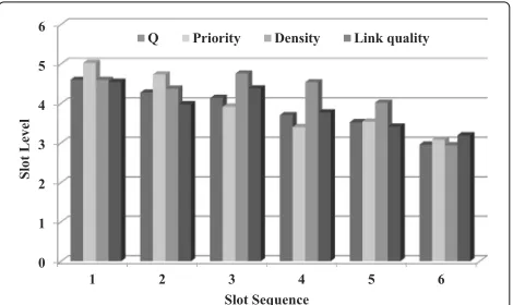
5.4 Simulation 4: transmission factor and cross-layer information in different time slots
Figure 12 shows the transmission factor, priority, neigh-bor node density, and link quality in all the six time slots. The horizontal axis describes the slot sequence, and the vertical axis describes the normalized slot level; the higher the slot level is, the larger the transmission factor, pri-ority, neighbor node density, and link quality are. As we can see in Fig. 12, the transmission factor decreases with the increase of the slot sequence which indicates the aver-age delay of the packets with a large transmission factor is lower than that of the other packets with a small trans-mission factor. Moreover, the priority of each time slot also decreases with the increase of the slot sequence.
Fig. 13Network throughput when each transmitter has different transmission chances
However, the downward trends of neighbor node density and link quality are not obvious because the influence to packet transmission of priority is higher than that of the other cross-layer information. From this figure, we can draw that the DTSMS protocol brings QoS improvement in system by considering the cross-layer information of transmitters.
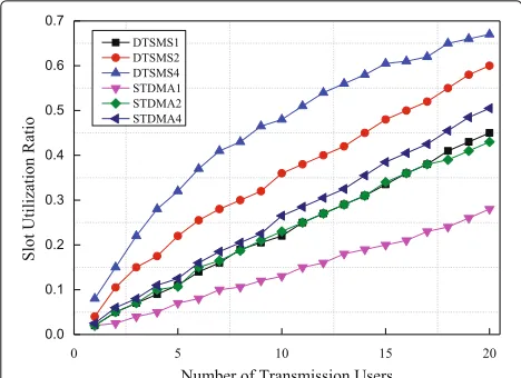
5.5 Simulation 5: slot utilization ratio with different transmission chances
This simulation evaluates the relationship of average throughput per slot and number of transmitting users. There are 40 transmitters in a contention area, and each transmission stream is 200 bytes in this simulation
scenario. The DOFMof each node is 4. We assume that every time slot is assigned to a proper time slot length to allow at most two transmission chances according to the QoS requirement. A cycle consists of all time slots allo-cated to nodes in a contention area, but only 20 nodes are transmitting and the other 20 nodes keep silence.
Figure 13 shows the average throughput per slot when each transmitter has 1, 2, and 4 transmission chances, respectively. In the STDMA protocol, each transmitter can use 4 DOFs to send data packets in their own slot without any collision. While in the DTSMS protocol, the transmitter not only sent data packets in their own slot but also allowed to send data packets in the unallocated slot when the slot is sensed to be idle. Therefore, the slot uti-lization ratio of DTSMS is higher than that of traditional STDMA.
5.6 Simulation 6: Overhead in DTSMS and TTS-MIMO
Figure 14 shows the overhead in DTSMS and TTS-MIMO. The horizontal axis describes the transmission time, and the vertical axis describes the overhead of DTSMS and TTS-MIMO. As we can see in Fig. 14, the overhead of DTSMS is higher than that of TTS-MIMO because of the dynamic nature in dynamic time slot allo-cation scheme. However, from another perspective, the increase of overhead in DTSMS seems acceptable in terms of the quality of service improvement.
6 Conclusions
Aiming to deal with the practical limitation in most of the MIMO MAC protocols, DTSMS protocol is proposed to improve the performance of the traditional STDMA in ad hoc networks. The DTSMS protocol highlights time slot
allocation and stream control scheme, which could sat-isfy the QoS requirement in terms of delay and support both unicast and multicast at the same time. Consider-ing the impact of cross-layer information, such as packet priority, neighbor node density, and link quality, DTSMS protocol decreases the delay of packets with higher trans-mission factor in ad hoc networks. The analysis and sim-ulation results show that the performance of DTSMS and TTS-MIMO are better than that of STDMA. Moreover, although the delay and overhead of DTSMS are higher than those of TTS-MIMO because of the dynamic nature of DTSMS, the throughput of DTSMS is also higher than that of TTS-MIMO, which is acceptable in terms of the QoS improvement.
Some other significant cross-layer information could influence the performance of our DTSMS protocol, such as channel state information (CSI). Therefore, taking the other important cross-layer information into comprehen-sive consideration will be part of our future work, which highlights the advantages of our DTSMS protocol.
Acknowledgements
This work was supported by the National Natural Science Foundation of China under Grant No. 61571350 and No. 61401334, the State Key Laboratory of Rail Transit Engineering Informatization (FSDI) (Contract No. SKLK16-06), the State Key Laboratory of Rail Traffic Control and Safety (Contract No. RCS2016K011), Beijing Jiaotong University, and the 111 Project (B08038).
Authors’ contributions
YS proposed the original idea, WY wrote the paper under the guidance of CL and LX, WY and CL designed the experiment and provided all of the figures, and LX checked the manuscript and contributed to the rearrangement of the materials. All authors read and approved the final manuscript.
Competing interests
The authors declare that they have no competing interests.
Publisher’s Note
Springer Nature remains neutral with regard to jurisdictional claims in published maps and institutional affiliations.
Author details
1State Key Laboratory of Integrated Services Networks, Xidian University, 710071 Xi’an, China.2State Key Laboratory of Rail Transit Engineering Informatization (FSDI), 710043 Xi’an, China.3State Key Laboratory of Rail Traffic Control and Safety, Beijing Jiaotong University, 100044 Beijing, China.
Received: 14 September 2016 Accepted: 15 May 2017
References
1. Y Song, J Xie, BRACER: a distributed broadcast protocol in multi-hop cognitive radio ad hoc networks with collision avoidance. IEEE Trans. Mobile Comput.14(3), 509–524 (2015)
2. M Hadded, P Muhlethaler, A Laouiti. IEEE Commun. Surv. Tutorials.17(4), 2461–2492 (2015)
3. W Zafar abd, B Khan. IEEE Technol. Soc. Mag.35(2), 67–74 (2016) 4. R Zi, X Ge, J Thompson, Energy efficiency optimization of 5G radio
frequency chain systems. IEEE J. Selected Areas Commun.34(4), 758–771 (2016)
5. T Bogale, L Le, Massive MIMO and mmWave for 5G wireless HetNet: potential benefits and challenges. IEEE Vehicular Technol. Mag.11(1), 64–75 (2016)
6. J Ni, H Xiao, Game theoretic approach for joint transmit beamforming and power control in cognitive radio MIMO broadcast channels. EURASIP J. Wireless Commun. Netw.2016(1), 98–107 (2016)
7. K Sundaresan, R Sivakumar, MA Ingram, T-Y Chang, Medium access control in ad hoc networks with MIMO links: optimization considerations and algorithms. IEEE Trans. Mobile Comput.3(4), 350–365 (2004) 8. Y Ma, A Yamani, N Yi, R Tafazolli, Low-complexity MU-MIMO nonlinear
precoding using Degree-2 Sparse Vector Perturbation. IEEE J. Selected Areas Commun.34(3), 497–509 (2016)
9. C Sun, X Gao, S Jin, M Matthaiou, Z Ding, C Xiao, Beam division multiple access transmission for massive MIMO communications. IEEE Trans. Commun.63(6), 2170–2184 (2015)
10. R Nelson, L Kleinrock, Spatial TDMA: a collision-free multihop channel access protocol. IEEE Trans. Commun.33(9), 934–944 (1985)
11. D Verenzuela, C Liu, L Wang, L Shi,Improving scalability of vehicle-to-vehicle communication with prediction-based STDMA. (IEEE Vehicular Technology Conference (VTC2014-Fall), Vancouver, 2014), pp. 1–5
12. F Hoffmann, D Medina, A Wolisz, Joint routing and scheduling in mobile aeronautical ad hoc networks. IEEE Trans. Vehicular Technol.62(6), 2700–2712 (2013)
13. J-S Park, A Nandan, M Gerla, H Lee,SPACE-MAC: enabling spatial reuse using MIMO channel-aware MAC. (IEEE International Conference on
Communication (ICC), Seoul, 2005), pp. 3642–3646
14. M Hu, J Zhang,MIMO ad hoc networks with spatial diversity: medium access control and saturation throughput. (IEEE Conference on Decision and Control (CDC), Nassau, 2004), pp. 3301–3306
15. M Park, S-H Choi, SM Nettles,Cross-layer MAC design for wireless networks using MIMO. (IEEE Global Telecommunications Conference (GlobeCom), St. Louis, 2005), pp. 2870–2874
16. P Casari, M Levorato, M Zorzi, MAC/PHY cross-layer design of MIMO ad hoc networks with layered multiuser detection. IEEE Trans. Wireless Commun.7(11), 4596–4607 (2008)
17. D Wang, U Tureli,Cross layer design for broadband ad hoc network with MIMO-OFDM. (IEEE 6th Workshop on Signal Processing Advances in Wireless Communications (SPAWC), New York, 2005), pp. 630–634 18. G Zhang, J Li, C Li, L Zhou, W Zhang, Topology-transparent reservation
time division multiple access in multihop ad hoc networks. Comput. Electr. Eng.32(6), 432–448 (2006)
19. W Mao, W Hamouda, I Dayoub,MIMO Cross-layer design for ad-hoc networks. (IEEE Global Telecommunications Conference (GlobeCom), Miami, 2010), pp. 1–5
20. OMF Abu-Sharkh,Cross-layer design for supporting infrastructure and ad-hoc modes integration in MIMO wireless networks. (Wireless Advanced (WiAd), London, 2011), pp. 110–115
21. W Ge, J Zhang, S Shen, A cross-layer design approach to multicast in wireless networks. IEEE Trans. Wireless Commun.6(3), 1063–1071 (2007)
22. I Hussain, Z Ahmed, D Saikia, A QoS-aware dynamic bandwidth allocation scheme for multi-hop WiFi-based long distance networks. EURASIP J. Wireless Commun. Netw.2015(1), 160–177 (2015)
23. R Andreotti, P Fiorentino, F Giannetti, V Lottici, Power-efficient distributed resource allocation under goodput QoS constraints for heterogeneous networks. EURASIP J. Adv. Signal Process.2016(1), 129–146 (2015) 24. J Hajipour, A Mohamed, V Leung, Utility-based efficient dynamic
distributed resource allocation in buffer-aided relay-assisted OFDMA networks. EURASIP J. Wireless Commun. Netw.2015(1), 263–283 (2007)
25. J Wang, Y Zhang, L Jiang,A novel time-slot allocation scheme for ad hoc networks with single-beam directional antennas. (IEEE International Conference on Communication Software and Networks (ICCSN), Chengdu, 2015), pp. 227–231
26. J Lunden, M Motani, H Vincent Poor,Distributed iterative time slot allocation for spectrum sensing information sharing in cognitive radio ad hoc networks.(IEEE Wireless Communications and Networking Conference (WCNC), Shanghai, 2013), pp. 29–34
27. M Nguyen, S Lee, S You, C Hong, L Le, Cross-layer design for congestion, contention, and power control in CRAHNs under packet collision constraints. IEEE Trans. Wireless Commun.12(11), 5557–5571 (2013) 28. R Arablouei, Recursive total least-squares algorithm based on inverse
power method and dichotomous coordinate-descent iterations. IEEE Trans. Signal Process.63(8), 1941–1949 (2015)
30. T Tanaka, Fast generalized eigenvector tracking based on the power method. IEEE Signal Process. Lett.16(11), 969–972 (2009)