Image Restoration without Information of Blur Operator using Blind Deconvolution

Available Online atwww.ijcsmc.com

International Journal of Computer Science and Mobile Computing

A Monthly Journal of Computer Science and Information Technology

ISSN 2320–088X

IJCSMC, Vol. 5, Issue. 1, January 2016, pg.127 – 132

Image Restoration without Information of

Blur Operator using Blind Deconvolution

Dhara Rana

Computer Department, MBICT, GTU, India

[email protected]

Abstract— before processing the captured images for further analysis, image restoration or removal of degradation from the image has become a great challenge for the researchers. Image restoration is the process of recovering the actual image from the blurred/degraded image. There are some direct and indirect techniques for image restoration. In direct techniques, image can be restored in a single step. While in indirect methods, image can be restored after a number of iterations. Problem of such method is that they require knowledge of the blur function that is Point Spread Function which is unknown. Number of methods has already been developed for image restoration. This paper presents various blurring methods and blind image de-convolution. Blind de-convolution restores the degraded image without the knowledge of distortion operator PSF. After several numbers of iterations, this method restores the degraded image efficiently.

Keywords—point spread function (PSF), Gaussian, optical transfer function (OTF)

I. INTRODUCTION

An image may be defined as 2D function g(x, y) where x and y are spatial coordinates and the amplitude of function at any pair of coordinates is called intensity or gray level of that image at that point. Image is the basic component of photography, video or any photo-editor software, remote sensing, satellite, medical science. Image is the main component of Image Processing field. Digital image processing is the processing of an image by means of computer. Image can be degraded due to shaky camera or motion blur, focusing problem, atmospheric effect, relative object camera motion etc. Image restoration is the process of recovering an original image from the degraded image. Image restoration sometimes refers to as image de-blurring or image deconvolution. Image consists of number of pixels and these all pixels have their intensity but when the intensity of a pixel in an image is spread over several pixels, image becomes blurred. The point/pixel is called point spread function (PSF) or blurring operator or blur function or blur kernel or distortion operator. Technically in spatial domain, point spread function (PSF) describes the degree to which an optical system blurs a point of light. The PSF is the inverse Fourier transform of Optical Transfer Function (OTF) in frequency domain. The OTF describes the response of a linear, positive-invariant system to an impulse in frequency domain. The OTF is the Fourier transform of the point spread function (PSF).

II. TYPESOFBLURSANDNOISE

an aspect of electronic noise. Noise may be added to image by medium through which it is created (random absorption or scatter effect), by recording medium (sensor noise/circuitry of scanner or camera) or by quantization of data for digital storage during acquisition or transmission. Noise is unwanted signal that adds unnecessary extra information in image.

In digital images various types of blur effects and noise effects exist:

Gaussian blur – blur an image with a Gaussian function. Convolution of image with Gaussian function results in Gaussian blur in the image. Sometimes Gaussian blur acts as a low pass filter since Gaussian blur reduces

high frequency components of image

.

Motion blur – when the image being recorded changes during the recording of a single exposure, either due to rapid movement or long exposure.

Out of focus blur – results if light from object points is not well converged. A. Types of Noise

Gaussian noise / Amplifier noise- additive in nature and follow Gaussian distribution means that each pixel in noisy image is sum of the true pixel value and a random Gaussian distributed noise value. The noise is independent of intensity of pixel value at each point. Gaussian noise is white noise which is normally distributed. Blurring effect is dense in the center and reduces towards the edges.

The probability density function of a Gaussian random variable is given by:

where represents the grey level, the mean value and the standard deviation and PG(z) is the Gaussian

distributed noise in the image[1]. Mean filter is good.

Poisson noise / Shot photon noise – Poisson/shot noise is the noise that can be introduced when number of photons sensed by the sensor is not sufficient to provide detectable statistical information. This noise has root mean square value proportional to square root intensity of image [2]. Different pixels are affected by independent noise values.

Salt–n-pepper noise / Impulse noise / binary noise – this type of degradation can be generated by sharp, sudden disturbances in the image signal, bit errors in transmission or analog-to-digital converter errors. Its appearance is randomly scattered white or black or both pixels over the image. Sometimes called spike noise or Fat-tail distributed noise.

Quantization noise / Uniform noise - The noise caused by quantizing the pixels of a sensed image to a number of discrete levels is known as quantization noise. It has an approximately uniform distribution. Mean filter is good for such noise.

Film grain - The grain of photographic film is a signal-dependent noise, with similar statistical distribution to shot noise. If film grains are uniformly distributed (equal number per area), and if each grain has an equal and independent probability of developing to a dark silver grain after absorbing photons, then the number of such dark grains in an area will be random with a binomial distribution. In areas where the probability is low, this distribution will be close to the classic Poisson distribution of shot noise [1]. Film grain is usually regarded as a nearly isotropic (non-oriented) noise source.

III.IMAGEDEGRADATIONANDRESTORATION MODEL

Original image f(x,y) is degraded by convolution of original image with the degradation filter/function h(x,y) and additive noise which results into g(x,y). Degradation function may be motion blur, out of focus, light scattering effect etc. Degraded image g(x,y) is passed to restoration filter which produces estimate of original image.

Figure 1. Image Degradation and Restoration Model [10]

Above model can be expressed mathematically as g(x,y) = h(x,y) * f(x,y) + ƞ(x,y) which shows that original image f(x,y), degraded image g(x,y) and noise ƞ(x,y) are coupled linearly. In this model, problem of recovering original image is known as linear image restoration problem. This problem assumes that the PSF is known in

advance

.

In many cases the PSF is unknown and therefore existing linear image restoration techniques are not applicable. For such cases blind image de-convolution can be used which restores the original image without any information about PSF.

IV.IMAGERESTORATIONTECHNIQUES

Image restoration methods can be categorized in two ways:

Without PSF- blind image deconvolution- in which blurring operator kernel is unknown that means image recovery is performed without degrading Point Spread Function which is more difficult. Blind image deconvolution method can be used effectively when no information about the distortion like blurring or noise is given. Blind de-convolution is used for blur detection and image restoration.

With PSF – inverse filtering, weiner filtering, LR filtering (Lucy-Richardson) – in which blurring operator kernel is known.

Out of all above image restoration techniques, blind image de-convolution is discussed in next section.

A. Blind Image Deconvolution

In this method the distortion operator is unknown. Distortion operator is Point Spread Function which has to be estimated. First step is to blur the image using Gaussian filter. Since the Fourier transform of a Gaussian is another Gaussian, applying a Gaussian blur has the effect of reducing the image's high-frequency components; a Gaussian blur is thus a low pass filter [10]. Gaussian filter is nonnegative. Additive noise, introduced during image equation, can be added explicitly into the filtered image. Result will be the blurred noisy image. Now this blurred image is used as an input to blind image de-convolution algorithm to obtain the estimated original image and estimated point spread function. Following are the steps to blur an image.

Step 1 Blur the input image using Gaussian blur function h(x,y)

Step 2 Apply Gaussian blur to the original image f(x,y) by convolving it with Gaussian function h(x,y) created in the previous step

g(x,y) = f(x,y) * h(x,y)

g(x,y) =

∑

m,n

Step 3 Add noise ƞ(x,y) to the Gaussian blurred image h(x,y) * f(x,y)

Step 4 Result is the degraded image g(x,y)

Following are the steps towards the Blind De-convolution of a blurred image.

Step 1 Initialize the parameters with values required for blind de-convolution

Weighted array is calculated. By default, WEIGHT is a unit array, the same size as the input image. Values between 0.0 and 1.0 can be assigned to elements in the WEIGHT array. The value of an element in the WEIGHT array determines how much the pixel at the corresponding position in the input image is considered. For example, to exclude a pixel from consideration, assign it a value of 0 in the WEIGHT array [11].

Random iteration value can be taken for algorithm to iterate for some number of times.

Blind de-convolution algorithm also requires an estimate of the PSF. This can be done on trial and error basis until good quality of the restored image is obtained.

Step 2 Apply Blind De-convolution for several numbers of iterations Step 3 Results are the restored degraded image and restored PSF

Step 4 Still restored Image is having ringing effects along its edges due to discrete Fourier transform used in the algorithm

Step 5 To remove this ringing effect, it is helpful to apply edgetaper function on the blurred input image first and then apply blind de-convolution algorithm

V. RESULTS

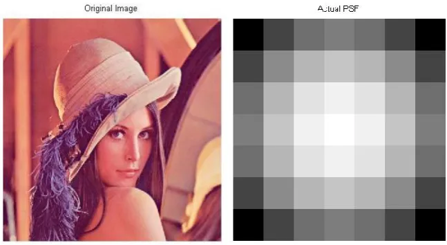
Image ‘lena.png’ of size 512 x 512 is used for experimental purpose.

Figure 4. Gaussian Blurred Image – Input to Blind Deconvolution Algorithm

Figure 5. Restored Image Figure 6.Restored PSF

VI.CONCLUSION

In this paper blind deconvolution has been studied for restoration of blur image. From the given result in the previous section, it can be stated that the blind de-convolution algorithm efficiently restores the blurred image without knowledge of distortion operator. Blind De-convolution for image restoration is studied in this paper. The Gaussian kernel is used to blur the input image. The ringing effect is removed by applying the edgetaper function which tapers the discontinuities along the blurred image edges. Then the blind de-convolution algorithm is applied to the output of edgetaper function to obtain restored image and restored point spread function. Thus without having information about distortion operator that is PSF and additive noise, blind image de-convolution algorithm efficiently restores the degraded image.

REFERENCES [1] https://en.wikipedia.org/wiki/Image_noise

[2] Minu Poulose, Literature Survey on Image Deblurring Techniques, International Journal of Computer Applications Technology and Research, Volume 2– Issue 3,pp. 286 - 288, 2013

[3] Dejee Singh, Mr R. K. Sahu, A Survey on Various Image Deblurring Techniques, International Journal of Advanced Research in Computer and Communication Engineering, Vol. 2, Issue 12, December 2013 ISSN (Print) : 2319-5940

[4] Mr. Rohit Verma , Dr. Jahid Ali, A Comparative Study of Various Types of Image Noise and Efficient Noise Removal Techniques, International Journal of Advanced Research in Computer Science and Software Engineering, Vol. 3, Issue 10, October 2013 ISSN: 2277 128X

[7] Anat Levin, Yair Weiss, Fredo Durand, William T. Freeman, Understanding and evaluating blind deconvolution algorithms, IEEE Conference on Computer Vision and Pattern Recognition, 2009 ISSN :1063-6919

[8] Bruno Amizic, Leonidas Spinoulas, Rafael Molina, Aggelos K. Katsaggelos, Compressive Blind Image Deconvolution, IEEE Transactions On Image Processing, Vol. 22, No. 10, October 2013

[9] Mariana S. C. Almeida, M´ario A. T. Figueiredo, Parameter Estimation for Blind and Non-Blind Deblurring Using Residual Whiteness Measures, IEEE Transactions On Image Processing, 2013