Efficient Generation of Power In Medium Voltage Direct Current Systems: Variable Speed Operation and Rectifier Considerations

University of South Carolina

Scholar Commons

Theses and Dissertations

1-1-2013

Experimental and Simulation Predicted Crack

Paths For AL-2024-T351 Under Mixed-Mode I/II

Fatigue Loading Using An Arcan Fixture

Eileen Miller

University of South Carolina - Columbia

Follow this and additional works at:https://scholarcommons.sc.edu/etd

Part of theMechanical Engineering Commons

This Open Access Dissertation is brought to you by Scholar Commons. It has been accepted for inclusion in Theses and Dissertations by an authorized administrator of Scholar Commons. For more information, please [email protected].

Recommended Citation

E

S

P

C

P

A

-2024-T351

M

-M

I/II

F

L

A

F

by

Eileen Miller

Bachelor of Science

University of South Carolina, 2011

Submitted in Partial Fulfillment of the Requirements

For the Degree of Master of Science in

Mechanical Engineering

College of Engineering and Computing

University of South Carolina

2013

Accepted by:

Michael A. Sutton, Director of Thesis

Xiaomin Deng, Co-director of Thesis

A

There are many people who have made this work possible for me. I would first

like to express my greatest appreciation for my advisor, Dr. Michael Sutton, for his

mentorship through my career at the University of South Carolina. He has provided

opportunities for me to work, learn, and grow as an engineer as well as proving support

educationally, financially, and personally. I would also like to thank Dr. Xiaomin Deng

for his guidance in this research project and in the classroom. His patience and

expectations of excellence have been invaluable to this work and my preparation for

future endeavors.

I would also like to extend my appreciation to Mr. Haywood Watts and Mr.

Brendan Croom for their assistance conducting experiments in the laboratory. Dr.

Anthony Reynolds provided valuable guidance in conducting the experiments, and Dan

Wilhelm played an instrumental role in troubleshooting with the test stand. Their help is

also greatly appreciated.

I also would like to acknowledge the financial support provided by NASA’s

South Carolina Space Grant Consortium through the Graduate Student Fellowship which

helped fund my education. Also the financial support provided by an Air Force Research

Lab SBIR project and specifically AFRL engineers Dr.. Robert Reuter and Dr. James

Harter is deeply appreciated. Finally, I would like to extend my thanks to the College of

Engineering and Computing at the University of South Carolina where the experiments

A

Mixed mode I/II fatigue experiments and simulations are performed for an Arcan

fixture and a 6.35mm thick Al-2024-T351 specimen. Experiments were performed for

Arcan loading angles that gave rise to a range of Mode I/II crack tip conditions from 0 ≤

∆KII/∆KI ≤∞. Measurements include the crack paths, loading cycles and maximum and

minimum loads for each loading angle. Simulations were performed using

three-dimensional finite element analysis (3D-FEA) with 10-noded tetrahedral elements via the

custom in-house FEA code, CRACK3D. While modeling the entire fixture-specimen

geometry, a modified version of the virtual crack closure technique (VCCT) with

automatic crack tip re-meshing and a maximum normal stress criterion was used to

predict the direction of crack growth. Results indicate excellent agreement between

experiments and simulations for the measured crack paths during the first several

T

C

ACKNOWLEDGEMENTS ... iii

ABSTRACT ... iv

LIST OF TABLES ... vii

LIST OF FIGURES ... viii

LIST OF SYMBOLS ... xi

LIST OF ABBREVIATIONS ... xvi

CHAPTER 1INTRODUCTION ...1

1.1 MOTIVATION ...1

1.2BACKGROUND ...3

1.3CURRENT WORK...10

CHAPTER 2EXPERIMENTAL WORK ...12

2.1FIXTURE AND SPECIMEN PREPARATION ...12

2.2SETUP ...14

2.3EXPERIMENTAL PROCEDURE ...16

2.4LOAD PREDICTION ...18

2.5DETERMINATION OF EXPERIMENTAL CRACK PATHS ...21

2.6EXPERIMENTAL RESULTS ...26

CHAPTER 3THEORETICAL WORK ...32

3.1CRACK3D ...32

3.3SIMULATION PROCEDURE ...42

3.4POST-PROCESSING OF SIMULATION RESULTS ...44

3.5THEORETICAL RESULTS ...44

CHAPTER 4DISCUSSION ...50

4.1DISCUSSION OF EXPERIMENTAL RESULTS ...50

4.2DISCUSSION OF THEORETICAL RESULTS ...52

CHAPTER 5CONCLUSIONS ...60

CHAPTER 6RECOMMENDATIONS FOR FUTURE WORK ...62

REFERENCES ...65

APPENDIX A–EXPERIMENTAL DATA RECORDED ...69

APPENDIX B–DETAILS AND TIPS FOR CRACK3DINPUT FILES GENERATION ...91

L

T

Table 2.1 Scale factors used to convert digitized points from pixels to meters ...25

Table 2.2 Percent error in crack path position ...25

Table 3.1 Table of applied displacements for line on top fixture ...41

Table 3.2 All combinations of simulations performed to verify convergence of solution 43 Table A.1. Experimental data recorded data for Φ = 15°. ...69

Table A.2. Experimental data recorded data for Φ = 30°. ...73

Table A.3. Experimental data recorded data for Φ = 45°. ...82

Table A.4. Experimental data recorded data for Φ = 60°. ...87

L

F

Figure 1.1 The three fracture modes for nominally elastic conditions ...3

Figure 1.2 A schematic of a typical log-log plot of Paris’ Law ...5

Figure 1.3 Diagram of Arcan fixture and specimen ...7

Figure 1.4 Specimen for Arcan fixture with single edge crack ...7

Figure 1.5 Schematic of kinked crack...8

Figure 2.1 Mixed mode I/II Arcan test fixture and butterfly shaped test specimen. Angle Φ = 0° corresponds to far-field tension and Φ = 90° is far-field shear ...13

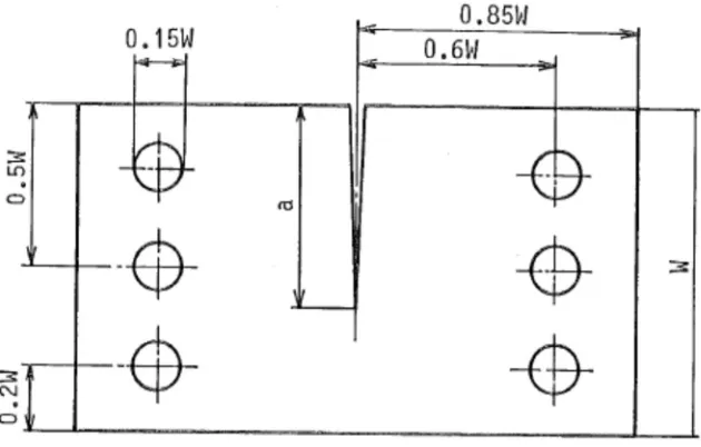
Figure 2.2 (a) Dimension of specimens in inches (b) Diagram of notch and pre-crack ....13

Figure 2.3 Images of experimental set up for 45° loading angle ...14

Figure 2.4 (Top) One degree-of-freedom slide apparatus; (Bottom) Two degree-of-freedom slide apparatus ...15

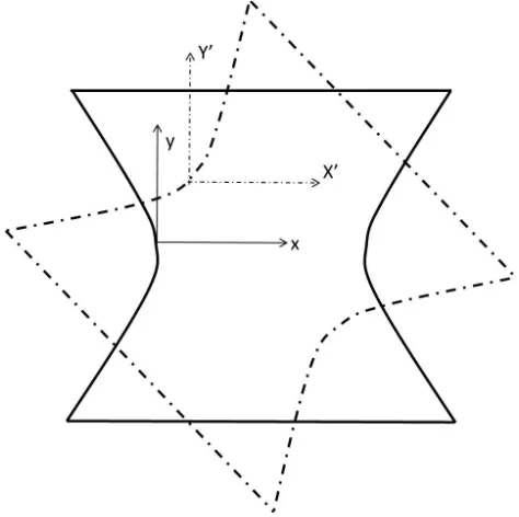
Figure 2.5 Schematic of coordinate system in which the crack tip was tracked during Pre-cracking (solid line) and testing (dotted line)...17

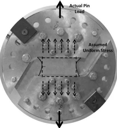
Figure 2.6 Visual representations of the actual geometry and loading (solid line) And the assumed geometry and loading (dotted lines) ...18

Figure 2.7 Diagram of geometry for Tada’s empirical expression ...19

Figure 2.8 Schematic of the images digitized and an exaggerated view of how the points Were selected for determining the scale factor from pixels to meters ...22

Figure 2.9 Coordinate system used to define crack paths from the tip of the pre-crack ...25

Figure 2.10 Crack growth rate along crack path for 30° loading case ...26

Figure 2.11 Crack growth rate along crack path for 45° loading case ...27

Figure 2.13 Originally digitized crack path data for 15° loading case ...28

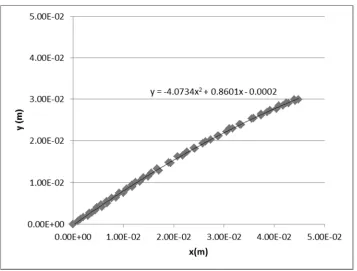
Figure 2.14 Digitized crack path and polynomial fit for 15° loading case ...29

Figure 2.15 Digitized crack path and polynomial fit for 30° loading case ...29

Figure 2.16 Digitized crack path and polynomial fit for 45° loading case ...30

Figure 2.17 Digitized crack path and polynomial fit for 60° loading case ...30

Figure 2.18 Crack path for Φ = 60° determined by slide apparatus experimentally versus the crack path determined by digitization ...31

Figure 3.1 An exaggerated local 2D view of a crack-front finite element mesh on the Plane normal to the crack-front, where the rigid springs between the node pairs have Zero length ...34

Figure 3.2 A local view of a crack front mesh on the extended crack surface, where the Local coordinate system for a mid-node on the crack front has its origin at the node 35 Figure 3.3 Diagram of crack growth direction for MCS criterion ...37

Figure 3.4 Diagram of a picture of actual Arcan fixture and specimen (left) and image of Finite element model geometry (right) ...39

Figure 3.5 Image of the 3D mesh ...40

Figure 3.6 A 2D view of the initial 3D finite element mesh in the specimen region ...40

Figure 3.7 Boundary conditions at Φ = 30° ...41

Figure 3.8 Crack path for Φ = 15° with various initial meshes, minimum element sizes, And crack increments ...45

Figure 3.9 2D view of the 3D deformed mesh for Φ = 45° (top) and a close up of the Crack path and re-meshing zone around the crack front ...45

Figure 3.10 The experimental and predicted crack path for the 15° loading case ...46

Figure 3.11 The experimental and predicted crack path for the 30° loading case ...46

Figure 3.12 The experimental and predicted crack path for the 45° loading case ...47

Figure 3.14 Plot of ∆KI and ΔKII along the crack path for the 15° loading case ...48

Figure 3.15 Plot of ∆KI and ΔKII along the crack path for the 30° loading case ...48

Figure 3.16 Plot of ∆KI and ΔKII along the crack path for the 45° loading case ...49

Figure 3.17 Plot of ∆KI and ΔKII along the crack path for the 60° loading case ...49

Figure 4.1 Plot of crack path for Φ = 30° and edge of top fixture ...51

Figure 4.2 Plot of ∆Keq and da/dN along crack length for 30° loading case ...56

Figure 4.3 Plot of ∆Keq and da/dN along crack length for 45° loading case ...57

Figure 4.4 Plot of ∆Keq and da/dN along crack length for 60° loading case ...57

Figure 6.1 Schematic of Arcan fixture with proposed tension bar for Φ = 75° ...64

L

S

σ

K Stress intensity factor.

KI Stress intensity factor for Mode I.

KII Stress intensity factor for Mode II.

KIII Stress intensity factor for Mode III.

σ Far field tensile stress.

a Crack length.

w Specimen width.

∆K Difference in maximum applied stress intensity factor and minimum applied stress intensity factor for fatigue loading.

Kmax Maximum applied stress intensity factor for fatigue loading.

Kmin Minimum applied stress intensity factor for fatigue loading.

R Loading ratio, also known as R-ratio.

σmax Maximum applied far-field tensile stress for fatigue loading.

σmin Minimum applied far-field tensile stress for fatigue loading.

N Number of loading cycles.

da/dN Crack growth rate which is the differential amount of crack growth per number of stress cycles.

C Material and R-ratio dependent proportionality constant for Paris’ Law.

∆KTH Threshold ∆K. The value below which the fatigue crack will not propagate.

Kc Fracture toughness. The value which, if Kmax exceeds, rapid crack propagation

ensues and final fracture occurs.

FI Function of loading, geometry, and crack orientation for determining KI

empirically.

FII Function of loading, geometry, and crack orientation for determining KII

empirically.

t Specimen thickness.

P Pin load applied using Arcan fixture.

α Angle from the vertical direction to the first segment of a kinked crack.

β Angle from the first segment of a kinked crack to the second segment.

b Crack length for the second segment of a kinked crack.

Φ Loading angle for Arcan fixture.

h Distance from crack to uniform tensile stress for Tada’s empirical solution for KI.

∆Keq Equivalent ∆K for the mixed mode loading condition.

γ, Parameters for ∆Keq.

γ1, γ2

xi, f Φ The ith x-position in pixels of the crack path for the font of the specimen for

loading case Φ.

xi,bΦ The ith x-position in pixels of the crack path for the back of the specimen for

loading case Φ.

yi,f Φ The i

th

y-position in pixels of the crack path for the font of the specimen for loading case Φ.

yi,bΦ The i

th

y-position in pixels of the crack path for the back of the specimen for loading case Φ.

∆xiΦ The standard deviation in pixels for all the x-positions of the crack path for the

∆yiΦ The standard deviation in pixels for all the y-positions of the crack path for the

font of the specimen for loading case Φ.

sv,f Φ The average vertical scale factor used for converting crack path y-position from

pixels to meters for the front of the specimen for loading case Φ.

sh,f Φ The average horizontal scale factor used for converting crack path x-position from

pixels to meters for the front of the specimen for loading case Φ.

sv,bΦ The average vertical scale factor used for converting crack path y-position from

pixels to meters for the back of the specimen for loading case Φ.

sh,bΦ The average horizontal scale factor used for converting crack path x-position from

pixels to meters for the back of the specimen for loading case Φ.

∆sv,f Φ The standard deviation of the vertical scale factor used for converting crack path

y-position for the front of the specimen for loading case Φ.

∆sh,f Φ The standard deviation of the horizontal scale factor used for converting crack

path x-position for the front of the specimen for loading case Φ.

∆sv,bΦ The standard deviation of the vertical scale factor used for converting crack path

y-position for the back of the specimen for loading case Φ.

∆sh,bΦ The standard deviation of the horizontal scale factor used for converting crack

path x-position for the back of the specimen for loading case Φ.

Xi,f Φ The average ith x-position in meters of the crack path for the front of the

specimen for loading case Φ.

Xi,bΦ The average ith x-position in meters of the crack path for the back of the

specimen for loading case Φ.

Yi,f Φ The average ith y-position in meters of the crack path for the front of the

specimen for loading case Φ.

Yi,bΦ The average i

th

y-position in meters of the crack path for the back of the specimen for loading case Φ.

∆Xi,f Φ The standard deviation for the i

th

x-position in meters of the crack path for the front of the specimen for loading case Φ.

∆Xi,bΦ The standard deviation for the ith x-position in meters of the crack path for the

∆Yi,f Φ The standard deviation for the ith y-position in meters of the crack path for the

front of the specimen for loading case Φ.

∆Yi,bΦ The standard deviation for the ith y-position in meters of the crack path for the

back of the specimen for loading case Φ.

∆a/∆N Crack growth rate which is the discrete amount of crack growth per number of stress cycles.

Kx Spring constant assumed in VCCT used in calculating the force in the x-direction.

Ky Spring constant assumed in VCCT used in calculating the force in the y-direction.

Kz Spring constant assumed in VCCT used in calculating the force in the z-direction.

Fx Reaction force in the x-direction on each node on the crack front and the mid-

nodes attached to the element just ahead of the crack front in VCCT.

Fy Reaction force in the y-direction on each node on the crack front and the mid-

nodes attached to the element just ahead of the crack front in VCCT.

Fz Reaction force in the z-direction on each node on the crack front and the mid-

nodes attached to the element just ahead of the crack front in VCCT.

ux Nodal displacement in the x-direction.

uy Nodal displacement in the y-direction.

uz Nodal displacement in the z-direction.

GI Strain energy release rate for Mode I.

GII Strain energy release rate for Mode II.

GIII Strain energy release rate for Mode III.

E Young’s modulus of elasticity.

ν Poisson’s Ratio.

∆a Crack growth increment.

θc Angle which the crack will propagate according to MCS criterion.

L

A

3D-FEA ... 3 – Dimensional Finite Element Analysis

SIF ... Stress Intensity Factor

2D-DIC ... 2 – Dimensional Digital Image Correlation

VCCT ... Virtual Crack Closure Technique

MCS ... Maximum Circumferential Stress

LT ... Longitudinal-Transverse

MTS ... Material Test System

NASA ... National Aeronautics and Space Administration

CHAPTER

1

I

1.1MOTIVATION

The aerospace industry has experience with a range of structural failures, oftentimes

due to fatigue cracks in aircraft fuselage components that are exposed to relatively high

stress levels during cyclic loading effects incurred during repeated take-off and landing

events that lead to fatigue crack initiation at material defects and near stress

concentrations. One of the first incidents that raised public awareness occurred in April of

1988 when 18 feet of the fuselage ripped off one of Aloha Airlines’ Boeing 737s in

midflight. The cabin quickly decompressed resulting in one fatality and eight serious

injuries. The National Transportation Safety Board reported that undetected dis-bonding

and widespread fatigue damage between rivets led to the failure of a lap joint [1]. A few

months later, Continental Airlines found several 30 inch long cracks in a Boeing 737

aircraft in the same general area where damage occurred in the Aloha Airlines incident

[2].

Ten years later, in October 1998, structural fatigue cracks in the fuselage of a Boeing

737s were reported [3], prompting the Federal Aviation Administration to propose the

Airworthiness Directive [3]. The directive required aircraft with less than 60,000 flight

cycles to be inspected initially and then inspected again every 3,000 cycles. Furthermore,

75,000 cycles. Considering only Boeing 737s in the United States, the estimated cost of

the inspections could be up to $26 million per inspection cycle and $71 million for

modifications [3].

Despite the efforts of airlines and the Federal Aviation Administration to monitor

fatigue cracks in aging aircraft, the danger of structural failure in fuselages continues into

the 21st century. In 2009, fatigue at the top of the fuselage just in front of the vertical tail

fin caused a 12 inch hole to rip open midflight, causing decompression of the cabin and

an emergency landing of a Southwest Airline Boeing 737 [4]. Southwest Airline had

another fuselage failure during flight just two years later. A section near the top of the

fuselage, about five feet long and one foot wide, ripped off due to the sudden propagation

of fatigue cracks in the skin of the aircraft [5].

The presence of fatigue cracks is not exclusive to commercial jetliners. In 2004,

Lockheed Martin made the switch from titanium to aluminum for some structural features

of the F-35 [6]. In 2010, fatigue cracks were discovered on the bulkhead of a Lockheed

Martin ground test aircraft [6]. Although no structural failure occurred in these cases, the

presence of fatigue cracks must be monitored to avoid potential catastrophes.

In fact, fatigue cracks are expected to form in the fuselage of modern airplanes due to

repeated (a) pressurization and decompression of the cabin during every flight and (b)

loading effects during take-off and landing. Thus, the propagation of cracks into critical

joints continues to be an area of concern, especially since such propagation under

complex stress states is not completely understood. Although procedures are currently in

propagate and in which direction it would grow when subjected to various loading

conditions could save millions of dollars in premature inspection and repair, while also

identifying the severity of an existing flaw in an aero-structure.

1.2BACKGROUND

As noted in Section 1.1, flaws in aircraft components oftentimes are exposed to

complex stress states. For nominally elastic conditions, the crack tip stress states

generally are decomposed into three modes of loading which are shown schematically in

Figure 1.1. Mode I, the opening mode, is such that the crack surfaces move away from

Figure 1.1. The three facture modes for nominally elastic conditions.

each other and the material directly ahead of the crack is subjected to a dominant tensile

stress. Mode II, the in-plane sliding mode, is such that shear loading is applied parallel to

the direction of crack growth and the material directly ahead of the crack tip is subjected

designated either out-of-plane or transverse shear, with the crack surfaces moving parallel

to and across each other. Mode I crack tip conditions are generally the dominant

influence on fatigue crack propagation in most aerospace metallic components (e.g.,

aluminum, titanium).

Crack propagation under Mode I loading is reasonably well understood [7]. Using a

maximum circumferential stress (MCS) criterion, the predicted and actual crack

trajectories during fatigue loading are perpendicular to the local σθθ max direction where

σθθ max is the maximum circumferential stress ahead of the crack tip [8]. This direction

nominally coincides with the loading direction when local conditions are not influenced

by stress concentrations, material defections/inclusions, or other factors.

For high cycle fatigue, it is generally assumed that the far field stress remains linear

elastic, while the local stress also remains mostly linear elastic with a small plastic zone

around the crack tip (ideally, the plastic zone size would be no more than one tenth of the

thickness of the specimen). The stress intensity factor (SIF), K, is a value which describes

the magnitude of the local elastic stress field and is a function of the stress and geometry

of the structure and crack. For Mode I loading, KI is defined by [7]

= √ ( ⁄ ) [1.1]

where σ is the far field tensile stress; is the crack length; and ( ⁄ ) is a parameter

which depends on the geometry of the specimen and crack orientation. Since the loading

is cyclic for fatigue studies, the loading parameter, ∆K, is considered the driving force for

where max and min refer to the maximum and minimum applied values of K. Another

loading parameter that has been shown to be important in fatigue studies is the loading

ratio, also known as the R-ratio. The R-ratio is defined as

=

=

[1.3]

Therefore can be expressed as

= (1 − ) [1.4]

The use of ∆K as the primary driving force in high cycle fatigue was introduced by Paul

Paris in his pioneering work [9]. Paris’ Law defines the relationship between ∆K and the

differential amount of crack extension per stress cycle, da/dN, and is written;

= [1.5]

Paris’ Law parameters, and !, are determined experimentally for each material and

may or may not be dependent on the loading ratio, .

As shown in Figure 1.2, a typical plot of the fatigue crack propagation process has

three regions. Below threshold, _"#, the crack will not propagate. Then in region I, the

crack growth begins to transition to region II where crack propagation occurs in a manner

that is predicted by Eq 1.5. In region III, the crack growth again transitions as

approaches the fracture toughness, _$. When ≥ _$, rapid crack propagation ensues

until final fracture occurs.

Now consider the case where a crack is under mixed-mode loading, that is, under any

combination of two or more loading types (see Figure 1.1). For the combination of Mode

I and Mode II loading conditions, methods for obtaining a mixed-mode I/II stress state

experimentally when applying uniaxial tensile loading include (a) use of kinked cracks,

(b) use of cracks propagating away from a hole, and (c) use of an Arcan fixture [9-18].

Independent mixed mode loading studies by both Zhang et al. [10] and Lopez-Crespo

et al. [11] have used an Arcan fixture to statically load an existing crack while 2D digital

image correlation (2D-DIC) was used to determine KI and KII from measured

displacement fields around the crack tip for various degrees of Mode I/II loading. Zhang

et al. used an Arcan fixture with a through thickness edge notch as the one shown in

Figure 1.3. Lopez-Crespo et al. used the same fixture with a center notched specimen.

Experimental SIFs were compared to values obtained from empirical expressions for the

Arcan fixture. The edge cracked solution takes the following form [12] .

= %_'(& √ , = %_'(& √ [1.6]

where t is specimen thickness and FI and FII are provided graphically as a function of

model. First, it is only valid for a range of relatively large cracks. Secondly, it only

considers straight cracks. Finally, it is only valid for static cracks. Thus, this model can

only be used for determining the kinking angle for the initial crack propagation event.

Figure 1.3. Diagram of Arcan fixture and specimen.

Figure 1.4. Specimen for Arcan fixture with single edge crack.

For the case of a kinked crack under uniform tensile loading (see Figure 1.5), another

Figure 1.5. Schematic of kinked crack.

= √%(), +,,) , = √%(), +,,) [1.7]

-./01,2,34

.//01,2,345 =

6789: ;1 ;

-./<02,34

._//<_02,3

45 − cos 2)

-./A02,34

._//A_02,3 45−

:BC ;1 ;

-./D02,34

._//D_02,3 45

[1.8]

E./F02,34G∑ ./,I (2)034 A

JK

._//I_02,3

4G∑ .//,I (2)034 A

JK L MN O =1,3

[1.9]

E./F02,34G∑ ./,I (2)034 Q</A A

JK

._//I_02,3

4G∑ .//,I (2)034 Q</A A

JK L MN O = 2

[1.10]

where FI,nk and FII,nk for n=0, 1, and 2 and k=1, 2, and 3 are provided in a table for 0°≤β≤

180° [12]. Equation 1.7 is valid for 0 ≤,

≤ 0.2. Limitations to this model are that (a) it

is applicable to kinked cracks in an infinite plate, (b) b « a, and (c) the loading must be

distributed in such a way that uniform stress is applied to the region in which the crack is

located. [12]

Gaylon et al. [13] performed fatigue tests using the Arcan fixture. In this study, the

authors determined the crack growth trajectory for various degrees of mixed-mode I/II

loading. Their results indicate that the crack trajectory is curvilinear and the stress

provided by Murakami and discussed previously are not applicable to quantify the mixed

mode SIFs. Also, the measured crack trajectories suggest that for all combinations of

Mode I/II loading, the fatigue cracks propagate in a manner that was locally dominated

by KI, while no crack propagation occurred for the pure Mode II loading case. However,

there was such large scatter in the experimental data that it is difficult to definitively

identify the trends. One cause of the inconsistency in the results was determined to be the

three pin loading configuration used by the authors. It was suggested that future studies

use only one pin for fixing the Arcan fixture to the test stand [14]; the use of a single pin

is consistent with the work of Amstutz, Boone and others at the University of South

Carolina [13, 14, 18, 21-23].

Chao et al. [15] also used the Arcan fixture with the one-pin configuration to study

fatigue crack propagation under various mixed-mode loading conditions. Crack

trajectories were compared to stable tearing results obtained under mixed-mode

monotonic loading conditions. It was observed that cracks under fatigue loading

propagate in a local Mode I direction for all loading cases including pure Mode II, unlike

Gaylon’s results. In Chao’s studies, the amount of crack growth in fatigue for Φ=75o and

90o was quite small, indicating that the crack surfaces interfered after a small amount of

crack extension and impeded further crack growth. For stable tearing, after Mode II

loading becomes dominant, cracks in aluminum alloys tended to propagate in the local

shear direction; that is, approximately parallel to the direction of the pre-crack. This

transition from Mode I dominated crack growth to Mode II dominated crack growth

under stable tearing conditions is consistent with results obtained by Amstutz et al [16]

stable tearing crack growth. The results show that for most loading cases, where KII/KI, <

1, the crack propagates under local Mode I conditions. However, as KI approaches zero

and KII/KI reaches a critical value (Φ=75o and 90o for Al 2024-T351), the crack begins to

grow in Mode II. While this study included crack propagation, stable tearing occurs

outside of the linear elastic range, and results suggest that the Mode II component has

different effects in the linear elastic range than it does under elastic-plastic conditions.

Boljanovic [18] performed finite element analysis to model the results of Gaylon et

al. The crack trajectories were simulated using MSC/NASTRAN [19] in a step-by-step

method while applying the maximum circumferential stress (MCS) criterion to predict

crack trajectory. Results of Boljanovic’s work agree with Gaylon’s experimental crack

paths. However, the SIFs were not obtained at each step using the local crack tip field

data, but were determined analytically after the simulation was performed since the

step-by-step method of crack path prediction is quite time consuming. It is unclear if the

analytical solution for the SIFs accounted for curvilinear crack paths.

1.3CURRENT WORK

The objective of the current study is to (a) perform experiments and measure the

crack path and (b) perform simulations and predict the fatigue crack path in an aerospace

aluminum alloy undergoing applied, far-field mixed-mode I/II conditions. The Arcan

fixture will be utilized to achieve far-field mixed-mode I/II conditions in 6.35mm thick

Al-2024-T351 specimens. Crack paths, cycle count, and maximum and minimum loads

will be measured during experiments, with loading ranging from 0 ≤ KII/KI ≤ ∞.

Simulations will then be performed using 3D-FEA. Crack trajectories will be predicted

will be used to extend the crack. The whole fixture and specimen will be modeled using

10-noded tetrahedral elements. Predicted crack paths will be compared to the results

CHAPTER 2

E

W

2.1 FIXTURE AND SPECIMEN PREPARATION

The Arcan fixture shown in Figure 2.1 was used to achieve mixed-mode I/II loading

for discrete values of KII/KI in the range 0 ≤KII / KI ≤∞. The butterfly-shaped specimen

shown in Figure 2.1 is machined to have tight contact with the upper and lower grips

along all four straight, angled sides. Once tightly fitted into the grips, the specimen is

further tightened into place using ten small bolts; five on the top part of the fixture and

five on the bottom part. Around the edges of the stainless-steel grips are pairs of holes

located every 15o. With loading angle Φ defined as shown in Figure 2.1, the Φ = 0o pin

holes correspond to nominally Mode I crack conditions and the Φ = 90o pin holes

represent nominally Mode II crack loading conditions. The fixture was machined from

15-5PH stainless steel with Young’s modulus =2.07 x 1011 Pa and Poisson’s ratio = 0.30.

As shown in Figure 2.2, each butterfly-shaped specimen is 224.28 mm tall, 275.30

mm wide at the top and bottom of the specimen and 6.35mm thick. Each specimen is

manufactured from Al-2024-T351 to form an LT orientation crack configuration (crack

is along the transverse direction (T) and perpendicular to the rolling direction (L) in the

aluminum specimen) [20] with Young’s modulus = 7.11 x 1010 Pa and Poisson’s ratio =

center (see Figure 2.2). The front and back surfaces of the specimens were sanded with

600 grit sand paper before final sanding with 800 grit sandpaper to remove small surface

defects. Metal polish was used to create a mirror finish on the surfaces for visually

tracking crack tip progression during the experiment.

Figure 2.2. (a) Dimensions of specimens in inches (b) Diagram of notch and pre- crack

2.2 SETUP

As shown in Figure 2.3, a 50 kip (227 kN) servo-hydraulic Material Test System

(MTS) controlled by TestStar II software was used to apply tensile loads in displacement

control to the Arcan fixture and specimen. Stainless steel clevises were placed in the

hydraulic grips of the MTS test frame, and the fixture was attached with one pin on the

top and another pin on the bottom. . The top image of Figure 2.3 is of the complete test

set-up with (a) the specimen and Arcan fixture pinned into the clevises of the test stand

and (b) microscope objectives and slide apparatus for optical tracking of the propagating

crack tip clamped to the test stand. The bottom image of Figure 2.3 shows the set up

without the microscope objectives. The backing plate (not visible in Fig 2.3) is attached

Figure 2.3. Images of experimental set up for a 45o loading angle.

During testing, the crack tip was tracked using the microscope objective and the slide

apparatus. The objective is attached to the dual slide apparatus shown in Figure 2.4. The

dual slide apparatus was designed and constructed by Mr. Haywood Watts. The apparatus

consists of (a) a single, horizontally mounted manual screw driven slide manufactured by

Velmex with a digital caliper to provide a metric positional measurement, (b) a second

vertically-oriented Velmex slide with digital caliper that was mounted to the horizontal

slide. The microscope objective was then connected to the vertical slide. Both vertical

and horizontal slides operate independently, allowing for horizontal and vertical

measurements of the crack tip position during the fatigue process.

2.3 EXPERIMENTAL PROCEDURE

To mount the notched specimen into the Arcan fixture, it was first bolted into the top

and bottom Arcan fixtures that were held in place by a backing plate designed to connect

the top and bottom halves of the fixture and keep the assembly from moving during

installation of the specimen into the fixture, minimizing initial distortions/stresses in the

specimen prior to the experiment. The fixture-specimen-backing plate combination was

pinned to the upper clevis, rotated about the pin to align with the bottom clevis and then

the lower pin was put in place to fully install the specimen-fixture combination in the

MTS test stand. Initially, the specimen is oriented to be in the Mode I configuration.

Once fully installed, the backing plate is removed. Then, two sets of dual slide

apparatuses were clamped to the test stand – one for tracking the crack on the front of the

specimen and the other for tracking the crack on the back of the specimen. The calipers

attached to the slides were zeroed at the center of the notch on the edge of the specimen,

see Figure 2.5. After everything is in place, the specimens were fatigue pre-cracked an

additional 6.35mm for a total crack length of 12.7mm. Fatigue loading was applied in

force control according to the loads outlined in the following section at 10Hz.

After pre-cracking, the crack front was marked by cycling at a higher loading ratio

(R=0.8 or R=0.9), and at about 90% of the pre-crack load. Then the backing plate was

reattached to the fixture, the fixture was rotated in the test stand to the appropriate

loading angle (e.g. see Figure 2.5). Once the specimen-fixture combination is correctly

positioned for the specific loading angle, Φ, of interest, the backing plate was again

re-zeroed at the center of the notch along the edge of the specimen and the length of the

pre-crack was re-measured.

Figure 2.5. Schematic of coordinate system in which the crack tip was tracked during pre-cracking (solid line) and testing (dotted line)

Following the procedure outlined in the previous steps, a total of 6 experiments were

performed at loading angles Φ = 15o, 30o, 45o, 60o, 75o, and 90o, with Φ = 90o degrees

being nominally Mode II crack loading. For the loading cases Φ = 15o, 30o, and 45o, the

one degree of freedom slide apparatus was used for tracking the crack tip. The two degree

of freedom slide apparatus was built and used to track the crack tip for Φ = 60o, 75o, and

90o. Again, fatigue loading at 10Hz was applied in force control according to the loads

outlined in the following section. The crack tip position was measured approximately

2.4 LOAD PREDICTION

Load data was predicted for fatigue pre-cracking and testing based on the load

predictions for tests performed previously for NASA Langley Research Center and the

US Air Force [21]. Load shedding was performed to avoid the risk of initiating stable

tearing or formation of a large plastic zone at the crack tip. The loading ratio, R, and the

amplitude of ∆KI were held constant at 0.17 and 359 Pa*m1/2 respectively, by allowing

the load to decrease as the crack length increased.

Figure 2.6. Visual representation of the actual geometry and loading (solid lines) and the assumed geometry and loading (dotted lines).

The SIF was estimated using an empirical expression from Tada [22] that is valid for

a through-thickness edge crack under uniform uniaxial tension. It was assumed that the

an estimate for the uniform applied stress was obtained using the load applied at the pin

divided by the cross-sectional area of the specimen using the assumed width and actual

thickness, w = 152.4 mm and t = 6.35 mm.

Figure 2.7. Diagram of geometry for Tada’s empirical expression.

0_V4 = W;V_Xtan_;VX∗].^_;`;.];(/V)`].a^(67:BCbAc) D

89:b_Ac [2.1]

While performing the first experiment, which was for the 15o loading case, it was

observed that the crack path on the front of the specimen deviated from the crack path

measured on the back surface after a few millimeters of crack extension. These

observations led to the implementation of a different approach for load prediction to

avoid unusual crack propagation in future experiments. The goal of the modified

approach was to keep ∆K constant in order to avoid excessive plasticity in the crack tip

region, crack slanting, or crack tearing. Since the method for estimating the SIF was quite

crude, and did not account for the various loading angles and resulting KI and KII values,

it was determined that following Paris’ Law for the material was a more accurate method

of crack growth control for ∆Keq which is defined as follows [23];

de = f+ (1 − f)h();+ f6();+ f;(); [2.2]

where γ, γ1, andγ2 are parameters to be defined. Using ∆Keq and assuming that there is no

crack closure effect, the crack growth rate can be determined using Eq 1.5. That is, the

authors opted to maintain the same crack growth rate throughout the experiment.

For the next experiment, the 30o loading case, pre-cracking was performed according

to the loads originally predicted. However after the specimen was rotated, the new

method of determining the loading was performed. From the previous test data, it was

determined that a crack growth rate of ≈ 6 x 10-5 mm/cycle was a safe rate to run the

experiments and maintain nominally linear elastic conditions.. A loading ratio R = 0.4

was chosen for the experiment. This crack growth rate was maintained by allowing the

crack to grow until the rate increased to ≈ 8 x 10-5 mm/cycle. The load was then dropped

process was repeated to maintain an average crack growth rate of ≈ 6 x 10-5 mm/cycle

and therefore maintain a constant average ∆Keq during the experiment.

For loading angles 45o, 60o, 75o, and 90o, the new pre-cracking loads and method of

load shedding to control crack growth rate were recomputed to maintain an

approximately constant crack growth rate. In all the remaining experiments, R = 0.4.

Cycle count, crack growth, and load data for each experiment are provided in Appendix

A. Recall for experiments for Φ = 15°, 30°, and 45° only the one degree of freedom

horizontal uni-slide was used to visually track the crack so the recorded value in the

appendix is only the x position as shown in Figure 2.5. For Φ = 60°, x’ and y’ positions

are recorded and reported in the appendix. Recorded data for Φ = 75° is not reported

since the crack did not propagate after applying hundreds of thousands of load cycles

using the same loads as applied in the Φ = 60° experiment.

2.5 DETERMINATION OF EXPERIMENTAL CRACK PATHS

In order to obtain the experimental crack path for each loading case, images of the

front and back of each specimen were necessary after the fatigue tests were conducted.

The surfaces of each of the specimens had to be prepared so that when images were

obtained, the crack would be visible and there would be no reflection on the surface.

First, the surface was sanded with 600 grit sand paper to roughen the surface and remove

the mirror finish. Then dry pigment was rubbed into the crack. The surface was sanded

again to remove excess pigment on the surface, leaving the remaining pigment in the

A 2.5 Megapixel Point Grey CCD camera was positioned on a tripod to ensure that

images were taken perpendicular to the surface of the specimen. The specimen was

positioned, and two rulers were placed on the surface of the specimen – one vertically

and the other horizontally-- to provide a scale when the images were digitized. Images

were taken of the front and back surfaces, and loaded into GetData Graph Digitizer

software [24]. First, using the ruler, 5 points were created at position (X,Y) and 5 more

points were created at (X+1”, Y+1”) as shown in Figure 2.8.

The distance between each set of points for the front (f) and back (b) of specimens for

each loading case, Φ, were determined in pixels and averaged to be used for a scale

factor. For each specimen, the average value and the standard deviation of the vertical

and horizontal scale factors for each case for the front (back) , sv,fΦ± ∆sv,fΦ(sv,bΦ± ∆sv,bΦ)

and sh,fΦ± ∆sh,fΦ(sv,bΦ± ∆sv,bΦ) respectively, are given in Table 2.1. Then i points were

selected along the front and back crack paths for each loading case, (xiΦ, yiΦ)f and (xiΦ,

yiΦ)b, and exported to Microsoft Excel. It was assumed that the error associated with

selecting the points along the crack path was ∆xiΦ, ∆yiΦ≈ ±1 pixel. Points along the path

were converted from pixels to meters using the scale factor, to give metric positions (XiΦ,

YiΦ)f and (XiΦ, YiΦ)b.

ij _{= k}

lj∗ mj, nj = koj∗ pj [2.3]

The standard deviation for the front and back of each specimen associated with the crack

path position, (XiΦ, YiΦ)f and (XiΦ, YiΦ)b, was determined using error propagation for

multiplication [25]:

i_,qj _{= i}

,qj ∗ rstuv,w

x

u_v,wx y ;

+ stx

_,wx y ;

, n_,qj = n_,qj ∗ rstuz,w x

u_z,wx y ;

+ st{x

{_,wx y ;

i_,,j _{= i}

,,j ∗ rstuv,3

x

uv,3x y

;

+ stx

_,3x y ;

,n_,,j = n_,,j ∗ rstuz,3x

uz,3x y

;

+ st{x

{_,3x y ;

[2.4]

The percent error in the crack path for each loading case, Φ, is defined as the maximum

percent error of the XiΦ and YiΦ points on the front and back of the specimen and is as

|}N~}€ NNMNj _{= 2 ∗ 〈}tƒ,wx

ƒ,wx ,

tƒ,3x

ƒ,3x ,

t„,wx

„,wx ,

t„,3x

„,3x 〉 ∗ 100 [2.5]

and are reported in Table 2.2. As shown in Table 2.2, the estimated errors are small and

assumed to be negligible. From this point forward only the average crack path points will

be considered in analysis.

Using Microsoft PowerPoint, the images for the front and back of each specimen

were set to ≈ 50% transparency and layered on top of each other. It was observed that the

specimen was slightly rotated in a couple of those images. The images were rotated such

that the edges of the specimen in both images were aligned. Using the angle of rotation

used in Power Point to align the images, the crack paths corresponding to those images

were rotated by the same angle. Then, the average points for each specimen were

translated to the coordinate system shown in Figure 2.9. The X and Y points along the

crack for the front and back of each specimen were plotted, and a second order

polynomial was fitted to the data using least squares. To verify that the digitized crack

path was accurate, a plot of the polynomial fit was layered on top of the image of the

Table 2.1. Scale factors used to convert digitized points from pixels to meters.

Loading Case

Front Image Scale Factor (m/pixel x 10-5)

Back Image Scale Factor (m/pixel x 10-5)

Vertical Scale Horizontal Scale Vertical Scale Horizontal Scale

15° 6.44 ± 0.03 6.41 ± 0.02 6.43 ± 0.02 6.39 ± 0.01

30° 7.14 ± 0.05 7.09 ± 0.04 7.14 ± 0.06 7.13 ± 0.03

45° 6.50 ± 0.07 6.48 ± 0.02 6.56 ± 0.02 6.52 ± 0.02

60° 6.48 ± 0.02 6.51 ± 0.00 6.55 ± 0.01 6.52 ± 0.03

Table 2.2. Percent error in crack path position.

Loading Case Percent Error

15° 1.0%

30° 1.3%

45° 2.2%

60° 0.8%

For the cases where the two degree of freedom slide apparatus was used, the x and y data

points recorded during the experiment in the coordinate system shown in Figure 2.5 were

rotated and translated into the coordinate system in Figure 2.9, in addition to digitizing

the crack path.

2.6 EXPERIMENTAL RESULTS

For the experiments performed using the modified load prediction method of

controlling the crack growth rate, the discrete crack growth rate Δ_a/Δ_{N was plotted along}

the crack length a in Figures 2.10-2.12.

Figure 2.11. Crack growth rate along crack path for 45° loading case.

Figure 2.12. Crack growth rate along crack path for 60° loading case.

For loading cases 15°, 30°, 45°, and 60°, fatigue crack propagation occurred, and for

loading cases 75° and 90°, no crack propagation occurred. Figure 2.13 shows the

originally digitized crack path for the 15° loading case. Figure 2.14 shows the data for the

15° loading case crack path before crack slanting occurred along with the polynomial fit

of the specimens for the 30°, 45°, and 60° loading cases respectively along with the

polynomial fit for each data set.

Figure 2.14. Digitized crack path and polynomial fit for 15° loading case.

Figure 2.16. Digitized crack path and polynomial fit for 45° loading case.

The rotated and translated crack path determined experimentally using the two degree

of freedom slide apparatus and the digitized crack path for Φ = 60° were plotted in Figure

2.18 to verify the accuracy of the digitization process. The following plot shows that the

two methods of obtaining the experimental crack path are in good agreement with each

other. The calipers used for measuring the amount of travel of the slide and microscope

objective have an accuracy of 0.00127mm which results in less than 0.01% error in the

measuring process. Even though the digitized crack path for Φ = 60° had 0.8% error

(Table 2.2), the digitization process has more opportunity to induce error through

obtaining, aligning, digitizing, and scaling the images. While error in either path is

negligible, the process of directly measuring the crack tip location using the dual caliper

apparatus during the experiment is accurate, efficient, and has less opportunity for

inducing error.

CHAPTER

3

T

W

3.1 CRACK3D

CRACK3D is a three-dimensional finite element code first developed by the

University of South Carolina and later jointly by the University of South Carolina and

Correlated Solutions, Inc.. It is capable of simulating elastic-plastic stable tearing crack

extension and linear-elastic fatigue crack propagation, both with curved crack fronts and

curvilinear crack paths for mixed-mode conditions. Two methods of crack growth

simulations are available: nodal release and local re-meshing. Nodal release assumes that

the crack path is known prior to running the simulation and is useful in evaluating crack

growth events with known crack paths from experimental measurements or for what-if

design scenarios. In the case that the crack path is to be predicted, local re-meshing is

used to extend the crack [1] [2] [3]. For the case of fatigue crack propagation, there are

three steps to crack growth predictions: (1) will the crack grow? (2) in what direction will

it grow? (3) how far will it extend for a certain number of loading cycles or how many

loading cycles will be required to extend the crack by a certain amount?

For determining if the crack will propagate, ∆K > ∆KTH must be true as discussed in

Section 1.2._{CRACK3D can be used to evaluate ∆K, which can be used to check if ∆K >}

∆KTH is satisfied. Once this crack growth criterion is met, CRACK3D can be used to

the variations of stress intensity factors with the amount of crack growth, which can be

used to predict the number of loading cycles as a function of the amount of crack growth.

In CRACK3D the determination of stress intensity factors is done using the method

of three-dimensional virtual crack closure technique (3D-VCCT) [3] [1] [2] [4] [5],

whichis based on the approach of the strain energy release rate [6], which is the amount

of energy released per unit thickness per unit crack extension when new crack surfaces

are created during crack extension. The 3D-VCCT can be used in finite element

simulations to calculate accurately and efficiently the mixed-mode strain energy release

rates, GI, GII, and GIII, which are related to the mixed-mode stress intensity factors KI, KII,

and KIII. Since fatigue crack propagation often occurs under nominally linearly elastic

conditions, it is assumed that the amount of energy required to extend the crack a small

increment is the same as the amount of energy required to close the crack. In Mode I, the

work required to close the crack per unit thickness is equivalent to one half the nodal

force multiplied with the opening displacement. In VCCT, this product between the nodal

force and opening displacement is approximated by using the nodal force at nodes

immediately ahead of the crack front and the crack opening displacement at

corresponding nodes immediately behind the crack front from the same finite element

solution. Okada et al. [4] applied VCCT to three-dimensional analysis using tetrahedral

elements. Deng et al. [3] [1] [2] later adopted Okada’s 3D-VCCT for general crack

To illustrate the 3D-VCCT, consider crack growth simulations using the nodal release

option. The extended crack is created by separating the crack front and mid- nodes

attached to the element just ahead of the crack front into coincident nodal pairs. It is

assumed that these nodal pairs are connected with a stiff spring with length zero as shown

in Figure 3.1.

Figure 3.1. An exaggerated local 2D view of a crack-front finite element mesh on the plane normal to the crack front, where the rigid springs between the node pairs have zero length.

Stiff spring constants, Kx, Ky, and Kz, which are large but otherwise arbitrary values

set in the nodal release option, and the displacements, ux, uy, and uz, of the upper (+) and

lower (-) nodes are used to compute the forces, Fx, Fy, and Fz(Eq 3.1) for each node,

where the coordinate system is such that x is along the direction of crack extension, y is

perpendicular to crack extension, and z is through the thickness and tangent to the crack

front.

Figure 3.2. A local view of a crack front mesh on the extended crack surface, where the local coordinate system for a mid-node on the crack front has its origin at the node.

Figure 3.2 shows the view of the crack front through the thickness where l is one

elements length and elements 1, 2, and 3 only. S1, S2, and S3 are the areas of the sides of

the tetrahedral elements on the extended crack surface for elements 1, 2, and 3

respectively. Nodes 1, 2, and 3 are nodes located on the crack front where node 1 is

attached to elements 1, 2, and 3 and node 2 is only attached to element 1.

Some nodes, such as 1 in Fig. 3.2, share element surfaces therefore the resultant

forces, Fx, Fy, and Fzfor node 1, must be divided among the surfaces S1, S2, and S3. For

element surface 1,

Then for element surface 1, the 3-D strain energy release rates, GI, GII, and GIII, are

estimated by summing up the work required to close the nodal pairs on the element

surface and are expressed as [4]

 ≈_aŠ6_<∑ % {†{,  ≈ _aŠ6_<∑ % †,  ≈ _aŠ6_<∑ % ‰†‰ [3.3]

where uxi, uyi, and uzi are the relative displacements between the top and bottom crack

surfaces at nodes behind the crack front that correspond to nodal forces Fxi, Fyi, and Fzi for

i nodes attached to the element surface ahead of the crack front. Finally, the SIFs for

plane strain are related to strain energy release rates by

= W_67‘/A , = ±W_67‘//A , = ±W_;(6`‘);/// [3.4]

where E is Young’s modulus and ν is Poisson’s ratio. It is noted that the signs for KII and

KIII are the same as the signs of the relative displacements behind the crack front along

the x and z axes, respectively.

It is noted that the SIF values described above correspond to the maximum loading

value applied during a loading cycle. Once the SIFs for the maximum applied load are

predicted using the VCCT, the direction in which the crack will propagate is predicted

using MCS criterion [5]. The MCS criterion assumes that a crack will grow in the

direction, θc, that maximizes the local circumferential stress, σθθ, at a specified location

ahead of the crack tip. The local stress around the crack tip can be expressed as a function

of SIF and position with respect to the crack tip in polar coordinates (r,θ) (see Figure 3.3).

““ = 1

√2Ncos s ”

2y s(cos s”2y);−32 sin ”y

Figure 3.3. Diagram of crack growth direction according to the MCS criterion.

It can be shown that that σθθ is maximum or minimum when the shear stress σrθ is zero.

So setting σrθ from Eq 3.5 to zero

0 = ‡sin ” + (3 cos ” − 1)ˆ [3.6]

and solving for θ,

”$ = 2 tan76

— ˜

™F//F/±rsF//F/y A

`š ›

œ  ž

[3.7]

The root that maximizes σθθ gives θc as the direction in which the crack will extend [5].

To apply the VCCT in crack growth simulations using the local re-meshing option

(instead of the nodal release option), the local mesh immediately ahead and behind the

crack front must be properly structured, so that the local mesh immediately behind the

crack front can be viewed as being shifted by one element size from the local mesh

immediately ahead of the crack front, Therefore, once crack growth is determined to

occur along a certain direction with a certain increment, the new mesh around the new

zone around the new crack front) with equal number of elements behind the crack front

and ahead of the crack front. [3] [1] [2]

A fatigue crack growth rate model, such as the Paris’ Law, is used to determine how

many cycles it will take for the crack to grow the amount of crack extension chosen by

the user [7]. However, since mixed-mode conditions are considered, Δ_{K as presented in}

Chapter 1 is no longer Mode I. After KI, KII, and KIII are predicted, ∆KI, ∆KII, and ΔKIII

can be computed using Eq 1.2, and ∆Keq from Eq 2.2. Again, assuming that there is no

crack closure effect, the crack growth rate can be determined using a Paris-type Law as in

Eq 1.5.

3.2 GEOMETRY, MESH GENERATION, AND BOUNDARY CONDITIONS

The Arcan fixture and specimen were modeled as shown in Figure 3.4. The fixture

and specimen are connected by bolts. For simplicity, this fixture-specimen connection is

approximated by a continuous bond at the fixture-specimen boundary. To this end, the

bolts are not modeled and the fixture and specimen are treated as three solid regions with

different thicknesses. Also, the outside radius of the fixture in the model corresponds to

the radius of the center of the pin holes on the actual fixture.

An idealized through-thickness edge notch and pre-crack exactly 12.7mm long was

modeled as the initial crack in the exact geometric vertical center of the specimen and is

perfectly horizontal into the width of the specimen. Material properties for the fixture and

specimen are Young’s modulus = 2.07 x 1011 Pa and 7.11 x 1010 Pa and Poisson’s ratio =

0.30 and 0.33 respectively. Both materials are modeled as being elastic-plastic through

Figure 3.4. Diagram of a picture of actual Arcan fixture and specimen (left) and image of finite element model geometry (right).

The volumes were then meshed with 10 noded tetrahedral elements. Figure 3.5 shows

the initial mesh generated, and Figure 3.6 shows the initial three zones of the mesh. As

discussed in Section 3.1 for local re-meshing, structured elements were created one

element ahead and one element behind the crack front. Then a transition zone was created

from the structured element to the far field mesh. Elements in this zone should transition

from the local minimum element size to a maximum element size at the boundary of the

local re-meshing zone. The far-field mesh away from the local region can be coarse,

Figure 3.5. Image of the 3D mesh.

The first mesh shown in Figure 3.6 has two elements through the thickness. A second

refined mesh was generated with 4 elements through the thickness in the structured area

to check for convergence of the mesh.

For each loading angle, Φ, a set of lines (one on the top fixture and the other on the

bottom fixture) corresponding to the center of the pins were created on the surface of the

fixture model in the through-thickness direction. The boundary conditions were such that

the displacement of the bottom line was set to zero in the x and y directions (ux,&uy =0)

and only the z displacement specified was of the center point on the bottom line (uz=0).

The displacement of the corresponding top line had a magnitude of 1 x 10-3mm along the

direction of loading, Φ, as shown in Figure 3.7, which was decomposed into x and y

components (see Table 3.1).

Figure 3.7. Boundary conditions at Φ = 30°.

Table 3.1. Table of applied displacements for line on top fixture.

Loading Case Displacement in x direction (ux) [1 x 10-3 mm]

Displacement in y direction (uy) [1 x 10-3 mm]

15° -0.259 0.966

30° -0.500 0.866

45° -0.707 0.707

3.3 SIMULATION PROCEDURE

The initial finite element meshes were created using ANSYS 14 [9]. Mesh data for

both the initial and initial refined meshes was exported from ANSYS using the

“NWRITE” and “EWRITE” commands, and the files were named NODES.DAT and

ELEMS.DAT respectively according to the CRACK3D manual.

There are 3 input files for CRACK3D for simulations using the local re-meshing

option. The first file, CRACK3D.MSH, contains the mesh information. The second file,

CRACK3D.DAT, is used to define the analysis type, parameters for analysis, and

boundary conditions. The last file used only for local re-meshing, CRACK3D.GEO,

defines the boundary lines and surfaces in which the crack and re-meshing are contained.

Two CRACK3D.MSH and CRACK3D.GEO files were created. One set of files was

for the initial mesh with 2 elements through the thickness at the crack front, and the

second file was for the initial mesh with 4 elements through the thickness. MESH3D, a

preprocessor for CRACK3D, was used to generate the CRACK3D.MSH file from the

NODES.DAT and ELEMS.DAT files. CRACK3D.GEO was created with the help of

ANSYS macros created by Dr. Weiming Lan. Output from the macros was compiled in

Microsoft’s Notepad to create the CRACK3D.GEO file.

The CRACK3D.DAT file was created in Microsoft’s Notepad following the

CRACK3D manual. A different CRACK3D.DAT file was created for each of the loading

cases. The crack growth simulation was performed using local re-meshing for fatigue

crack growth with VCCT and the MCS criterion for crack growth direction prediction.

Parameters for Δ_{Keq defined in Eq 2.2 were chosen as follows: γ=0, γ1=1, γ2=1.Paris}

specific material and loading ratio being simulated were not currently available so that

parameters for a different R-ratio were input. Also, the minimum element size, maximum

element size, radius for the local re-meshing region, and increment for crack growth were

defined. Boundary conditions were input for the specific loading case as described above

in Section 3.2. As an example, the input files for the simulation for loading case Φ = 45°

are contained in Appendix C.

The first simulations were performed to check for convergence of the crack path. For

the 15° loading case, simulations were performed using the first initial mesh with 2

elements through the thickness and with the initial refined mesh containing 4 elements

through the thickness. The minimum element sizes equivalent to 1 /2 the thickness, 1 /4

the thickness, and 1/8 the thickness were used, and crack growth increments for 0.001m

and 0.002m were used. The maximum element size and re-meshing zone size remained

constant at 0.006m and 0.012m respectively. Table 3.2 shows all the combinations of

simulations performed to check convergence.

Table 3.2. All combinations of simulations performed to verify convergence of solution

Number of elements through thickness of initial

mesh

Minimum element size [m] Crack growth increment [m]

2

.003 0.001

0.002

.0015 0.001

0.002

4

.0015 0.001

0.002

.00075 0.001

0.002

Simulations were performed for loading cases Φ = 15°, 30°, 45°, and 60°. In some