Discrete time hands off control by sparse optimization

R E S E A R C H

Open Access

Discrete-time hands-off control by sparse

optimization

Masaaki Nagahara

, Jan Østergaard

and Daniel E. Quevedo

Abstract

Maximum hands-off control is a control mechanism that maximizes the length of the time duration on which the control is exactly zero. Such a control is important for energy-aware control applications, since it can stop actuators for a long duration and hence the control system needs much less fuel or electric power. In this article, we formulate the maximum hands-off control for linear discrete-time plants by sparse optimization based on the1norm. For this optimization problem, we derive an efficient algorithm based on the alternating direction method of multipliers (ADMM). We also give a model predictive control formulation, which leads to a robust control system based on a state feedback mechanism. Simulation results are included to illustrate the effectiveness of the proposed control method.

Keywords: Hands-off control, Sparse optimization, Discrete-time control, Optimal control, ADMM, Model predictive control, Green control

1 Introduction

Sparsity is one of the most important notions in recent sig-nal/image processing [1], machine learning [2], commu-nications engineering [3], and high-dimensional statistics [4]. A wide range of applications is shown in works, such as [5].

Recently, sparsity-promoting techniques have been applied to control problems as stated below. Ohlsson et al. have proposed in [6] sum-of-norms regularization for trajectory generation to obtain a compact representa-tion of the control inputs. In [7], Bhattacharya and Ba¸sar have adapted compressive sensing techniques to state esti-mation under incomplete measurements. The sparsity notion is also applied to networked control for reduc-tion of control data size using model predictive control (MPC) [8–10]. MPC is a very attractive research topic to which sparsity methods are applied; in [11, 12] Gallieri and Maciejowski have proposedasso-MPC to reduce actuator

activity, and in [13] Aguilera et al. have discussed min-imization of the number of active actuators subject to closed-loop stability by using the0 norm. Sparse MPC is further investigated based on self-triggered control in [14].

*Correspondence: nagahara@ieee.org

1Institute of Environmental Science and Technology, The University of Kitakyushu, Hibikino, 808-0135 Fukuoka, Japan

Full list of author information is available at the end of the article

Motivated by these researches, themaximum hands-off controlhas been proposed in [15, 16] for continuous-time systems. This control maximizes the length of the time duration over which the control value is exactly zero. With such control, actuators can be stopped for a long dura-tion, during which the control system requires much less fuel or electric power, emits less toxic gas such as CO2, and generates less noise. Therefore, the control is also calledgreen control[17]. The optimization is described as a finite-horizonL0_{-optimal control, which is}

discontinu-ous and highly non-convex, and hence difficult to solve in general. In [15, 16], under a simple assumption of nor-mality, theL0-optimal control is proved to be equivalent to classical L1-optimal (or fuel optimal) control, which can be described as a convex optimization. The proof of the equivalence theorem is mainly based on the “bang-off-bang” property (i.e., the control takes values±1 or 0 almost everywhere) of theL1-optimal control. Moreover, based on the equivalence, the value function in the max-imum hands-off control is shown to be continuous and convex in the reachable set [18], which can be used to prove the stability of an MPC-based closed-loop system.

In this paper, we investigate the hands-off control in discrete time for energy-aware green control. The main difference from the continuous-time hands-off control men-tioned above is that the discrete-time maximum hands-off control shows in many cases no “bang-off-bang” property.

Instead, we use the restricted isometry property (RIP), e.g., [3], for an equivalence theorem between0and1.

An associated 1-optimal control problem can be described via an1optimization problem with linear con-straints. This can be equivalently written as a standard linear program, which can be “efficiently” solved by the point method [19]. The efficiency of the interior-point method is true for small or middle-scale problems with offline computation. However, for real-time control applications, problems arise. To improve computational efficiency in the current paper, we adapt the alternating direction method of multipliers (ADMM) to the control problem. ADMM was first introduced in [20] in 1976, and since then, the algorithm has been widely investi-gated in both theoretical and practical aspects; see the review [21] and the references therein. ADMM has indeed been proved to converge to the exact optimal value under mild conditions, but in some cases it shows quite slow convergence to the optimal value. On the other hand, ADMM often gives very fast convergence to an approxi-matedvalue ([21], section 3.2). This property is desirable for real-time control application, since the approximation error can often be eliminated by relying upon robust-ness of the feedback control mechanism. In fact, ADMM has been applied to MPC with a quadratic cost func-tion in [22–24]. In particular, an ADMM algorithm for 1_{-regularized MPC has been proposed in [25] without}

theoretical stability results.

1.1 Contributions

In this paper, we first analyze discrete-time finite-horizon hands-off control, where we give a feasibility condition based on the system controllability, and also develop an equivalence theorem between0- and1-optimal controls based on the idea of RIP. These are different from the case of continuous-time hands-off control in [16], where the concept of normality for an optimal control problem was adopted. Unfortunately, normality cannot be used in the discrete-time case. RIP is often used to prove equiv-alence theorems, e.g., [1] in signal processing, and we show in this paper that RIP is also useful for discrete-time hands-off control.

To calculate discrete-time hands-off control, we then propose to use ADMM, which is widely applied to sig-nal/image processing [21], and we prove by simulation that ADMM is very effective in feedback control since it requires very few iterations. Finally, we prove a sta-bility theorem for hands-off model predictive control, which has been never given in the literature except for the continuous-time case [18].

1.2 Outline

The paper is organized as follows: in Section 2, we for-mulate the discrete-time maximum hands-off control, and

prove the feasibility property and the 0_-1 _equivalence

based on the RIP. In Section 3, we briefly review ADMM, and give the ADMM algorithm for maximum hands-off control. The penalty parameter selection in the optimiza-tion is also discussed in this secoptimiza-tion. Secoptimiza-tion 4 proposes MPC with maximum hands-off control, and establishes a the stability result. We include simulation results in Section 5, which illustrate the advantages of the proposed method. Section 6 draws concluding remarks.

1.3 Notation

We will use the following notation throughout this paper:

Rdenotes the set of real numbers. For positive integers nandm,Rn andRm×ndenote the sets ofn-dimensional real vectors and m× n real matrices, respectively. We use boldface lowercase letters, e.g.,v, to represent vectors, and upper case letters, e.g.,Afor matrices. For a positive integern,0ndenotes then-dimensional zero vector, that

is, 0n =[ 0,. . ., 0]∈ Rn. If the dimension is clear, the

zero vector is simply denoted by0. The superscript(·) means the transpose of a vector or a matrix. For a vector v=[v1,v2,. . .,vn]∈Rn, we define the1and2norms,

respectively, by

v1 n

k=1

|vk|, v2

n

k=1

|vk|2.

Also, we define the 0 norm of v as the number of nonzero elements ofvand denote it viav0. A vectorvis

calleds-sparse ifv0≤s, and the set of alls-sparse

vec-tors is denoted bys {v∈RN :v0≤s}. For a given

v ∈ RN, the1_{-distance fromvto the set}

sis defined

by

σs(v)min

x∈sv−x1.

We say a set is non-empty if it contains at least one ele-ment. For a non-empty set, the indicator operator for is defined by

I(x)

0, ifx∈, ∞, otherwise.

2 Discrete-time hands-off control

In this article, we consider discrete-time hands-off control for the following linear time-invariant model:

x[k+1]=Ax[k]+bu[k] , k=0, 1,. . .,N−1, (1)

where x[k]∈ Rn is the state at time k, u[k]∈ Ris the discrete-time scalar control input, andA∈Rn×n,b∈Rn. The control (sequence){u[0] ,u[1] ,. . .,u[N−1]}is cho-sen to drive the statex[k] from a given initial statex[0]=ξ to the originx[N]=0inNsteps.

in (1) with the boundary conditions,x[0]=ξandx[N]= 0, we obtainANξ+u=0with

AN−1bAN−2b . . .Ab b. (2)

By this, the feasible control setU_ξis represented by

Uξ= u∈RN :ANξ+u=0. (3)

For the feasible control setUξ, we have the following lemma.

Lemma 1. Assume that the pair(A,b)is reachable, i.e.,

rankb Ab . . . An−1b=n, (4)

and N>n. ThenU_ξis non-empty for anyξ ∈Rn_.

Proof.SinceN>n, the matrixin (2) can be written as

1 2

,

1

AN−1bAN−2b . . . Anb,

2

An−1bAn−2b . . . Ab b.

(5)

From the reachability assumption in (4),2is

nonsin-gular. Then the following vector

˜

u

0N−n

−−1 2 ANξ

, (6)

satisfiesANξ+u˜ =0, and henceu˜∈U_ξ.

For the feasible control setU_ξ in (3), we consider the discrete-time maximum hands-off control (or0-optimal control) defined by

minimize

u∈U_ξ u0, (7)

whereu = u[0] ,u[1] ,. . .,u[N−1], andu0is

so-called the0_{norm ofu, which is defined as the number}

of nonzero elements ofu. We call a vectorus-sparseif u0≤s. Letsbe the set of alls-sparse vectors, that is,

s{u∈RN :u0≤s}.

For the 0 optimization in (7), we have the following observation:

Lemma 2. Assume that the pair(A,b) is reachable and N>n. Then, we haveUξ∩n= ∅.

Proof.From the proof of Lemma 1, there exists a feasible controlu˜ ∈Uξ that satisfies ˜u0 ≤ n; see (6). It follows

thatu˜∈nand henceu˜∈Uξ∩n.

This lemma assures that the solution of the 0 opti-mization is at mostn-sparse. However, the optimization problem (7) is a combinatorial one, and requires heavy computational burden ifnorNis large. This property is undesirable for real-time control systems, and we propose

to relax the combinatorial optimization problem to obtain a convex one.

For this purpose, we adopt an1relaxation for (7), that is, we consider the following1-optimal control problem:

minimize

u∈U_ξ u1, (8)

whereu1|u[0]|+|u[1]|+· · ·+|u[N−1]|. The

result-ing optimization can be described as a linear program, and hence we can solve it efficiently by using numerical software such asCVX inMATLAB[26, 27]. Moreover, an accelerated algorithm is derived by the alternating direc-tion method of multipliers (ADMM) [21]; see Secdirec-tion 3.

To justify the use of the 1 relaxation, we recall the restricted isometry property[1] defined as follows: Definition 1. A matrixsatisfies the restricted isometry property (RIP for short) of order s if there existsδs ∈(0, 1)

such that

(1−δs)u22≤ u22≤(1+δs)u22

holds for allu∈s.

Then, we have the following theorem.

Theorem 1. Assume that the pair(A,b)is reachable and that N > n. Suppose that the0 optimization (7) has a unique s-sparse solution. If the matrixgiven in (2) satis-fies the RIP of order2s withδ2s<

√

2−1, then the solution of the1-optimal control problem (7) is equivalent to that of the0-optimal control problem (8).

Proof.Letu∗denote the uniques-sparse solution to (7). By ([28], Theorem 1.2) or ([1], Theorem 1.8), the solution to the1optimization (8), which we denote byuˆ, obeys

ˆu−u∗2≤C0σs(

u∗) √

s ,

whereC0is a constant given by

C0=2·

1−(1−√2)δ2s

1−(1+√2)δ2s

,

and

σs(u∗)min v∈su

∗_−v

1.

Sinceu∗iss-sparse, that is,u∗∈s, we haveσs(u∗)=0,

and henceuˆ=u∗.

3 Numerical optimization by ADMM

Although ADMM generally only achieves very slow con-vergence to the exact optimal value, it is shown in ([21], Section 3.2) that ADMM often converges to modest accu-racy within a few tens of iterations. This property is especially favorable in model predictive control, since the computational error generated by the ADMM algorithm can often be reduced by the feedback control mechanism; see the simulation results in Section 5.

3.1 Alternating direction method of multipliers (ADMM)

Here, we briefly review the ADMM algorithm. ADMM is an algorithm to solve the following type of optimization:

minimize

y∈Rμ,z∈Rν f(y)+g(z) subject to Cy+Dz=c (9)

wheref : Rμ → R∪ {∞}andg : Rν → R∪ {∞}are closed and proper convex functions, andC ∈Rκ×μ,D∈

Rκ×ν_{,c ∈ R}κ_{. For this optimization problem, we define}

theaugmented Lagrangianby

Lρ(y,z,w)f(y)+g(z)+w(Cy+Dz−c)

+ρ

2Cy+Dz−c

2 2,

(10)

whereρ >0 is called the “penalty parameter” (or the step size; see the third line of the ADMM algorithm below). Then the algorithm of ADMM is described as

y[j+1] :=arg min

y∈Rμ

Lρ(y,z[j] ,w[j]),

z[j+1] :=arg min

z∈Rν Lρ(y[j+1] ,z,w[j]),

w[j+1] :=w[j]+ρCy[j+1]+Dz[j+1]−c, j=0, 1, 2,. . .,

(11)

where ρ > 0,y[0]∈ Rμ,z[0]∈ Rν, andw[0]∈ Rκ are given before the iterations.

Assuming that the unaugmented LagrangianL0(i.e.,Lρ

with ρ = 0) has a saddle point, the ADMM algorithm is known to converge to a solution of the optimization problem (9) ([21], Section 3.2).

3.2 ADMM for1_{-optimal control}

Here we derive the ADMM algorithm for the1-optimal control (8). The optimization (8) can be described in the standard form in (9) as follows:

minimize

y,z∈RN IUξ(y)+ z1 subject to y−z=0,

whereI_Uξis the indicator operator forUξ, that is

IUξ(y)

0, ify∈Uξ, ∞, otherwise.

Then, the ADMM algorithm for the1_{-optimal control (8)}

is given by

y[j+1] :=(z[j]−w[j]),

z[j+1] :=S1/ρ(y[j+1]+w[j]),

w[j+1] :=w[j]+y[j+1]−z[j+1] , j=0, 1, 2,. . ., (12)

whereis the projection operator ontoUξ, that is,

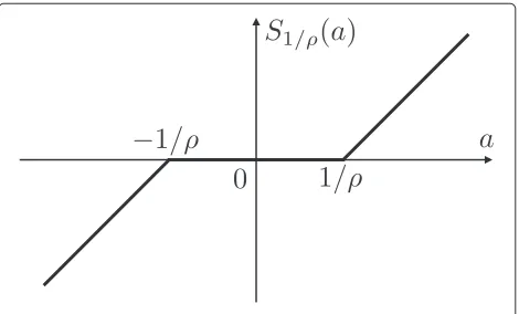
(v)I−()−1v−()−1ANξ, (13) is as in (2), andS1/ρ is the element-wise soft

thresh-olding operator (see Fig. 1) defined by (for scalars a)

S1/ρ(a)

⎧ ⎨ ⎩

a−1/ρ, ifa>1/ρ, 0, if|a| ≤1/ρ, a+1/ρ, ifa<−1/ρ.

(14)

The operatorS1/ρ is also known as the proximity oper-ator for the1_{-norm term in the augmented Lagrangian}

L_ρ. Note that if the pair (A,b) is reachable and N > n, then the matrix is full row rank (see the proof of Lemma 1), and hence the matrix is non-singular. Note also that the matrixI−()−1and the vector ₍₎−1_AN_{ξin (13) can be computed before the}

iter-ations in (12), and hence the computation in (12) is very simple.

3.3 Selection of penalty parameterρ

To use the ADMM algorithm in (12), we should appro-priately determine the penalty parameter (or the step size) ρ. In general, if the penalty parameter is large, then the primal residualy[j]−z[j], orCy[j]+Dz[j]−c[j] tends to be small, since it places a large penalty on violations of primal feasibility; see (10). On the other hand, a smaller ρ tends to give a sparser output from the definition of the soft thresholding operatorS1/ρ; see

(14) or Fig. 1. For the selection of ρ, one should rely on trial and error by simulation. One may extend the

idea of optimal parameter selection for quadratic prob-lems [24, 30] to the 1 optimization (8), for which we do not have any optimal parameter selection method. Alternatively, one can adopt thevarying penalty param-eter ([21], Section 3.4), in which one may use possibly different penalty parametersρ[j] for each iteration. See also [31, 32].

4 Model predictive control

Based on the finite-horizon1-optimal control in (8), we here extend it to infinite-horizon control by adopting a model predictive control strategy.1

4.1 Control law

The control law is described as follows. At timek (k = 0, 1, 2,. . .), we observe the statex[k]∈Rn_{of the}

discrete-time plant (1). For this state, we compute the1_-optimal

control vector

ˆ u[k]

⎡ ⎢ ⎢ ⎢ ⎣

ˆ u0[k]

ˆ u1[k]

.. . ˆ uN−1[k]

⎤ ⎥ ⎥ ⎥

⎦arg minu∈Uξ

u1, ξ=x[k] .

(15)

Then, as usual in model predictive control [33, 34], we use the first elementuˆ0[k] for the control inputu[k], that

is, we set

u[k]= ˆu0[k]=[1 0 . . . 0]uˆ[k] . (16)

This control law gives an infinite-horizon closed-loop control system characterized by

x[k+1]=Ax[k]+Buˆ0[k] . (17)

Since the control vectoruˆ[k] is designed to be sparse by the1optimization as discussed above, the first element,

ˆ

u0[k], will often be exactly 0, e.g., the vector shown in

(6). A numerical simulation in Section 5 illustrates that the control will often be sparse, when using this model predictive control formulation.

4.2 Stability

We here discuss the stability of the closed-loop system (17) with the model predictive control described above. In fact, we can show the stability of the closed-loop con-trol system by using a standard argument in the stability analysis of model predictive control with a terminal con-straint (e.g., ([33], Chapter 6), ([34], Chapter 2), or ([35], Chapter 5)).

The key idea of the stability analysis in model predictive control is to use thevalue functionof the (finite-horizon) optimal control problem as a Lyapunov function. The

value function of the1_{-optimal control in (8) is defined}

by (see (15))

V(ξ)min

u∈Uξu1. (18)

The following lemma shows the convexity, the conti-nuity, and the positive definiteness of the value func-tionV(ξ). These properties are useful to show the value function to be a Lyapunov function (see the proof of Theorem 2 below).

Lemma 3. Assume that the pair (A,b) is reachable, A is nonsingular, and N > n. Then V(ξ) is a convex, continuous, and positive definite function onRn.

Proof.First, we prove convexity. Fix initial statesξ,η ∈

Rn_{and a scalarλ∈(0, 1). From Lemma 1, there exist}1

-optimal controlsuˆξanduˆηforξandη, respectively. Then the controlν λuˆξ +(1−λ)uˆηis feasible for the initial stateζ λξ+(1−λ)η, that is,ν∈Uζ. From the convexity of the1norm, we have

Vλξ+(1−λ)η≤ ν1=λuˆξ+(1−λ)uˆη₁

≤λ ˆuξ1+(1−λ) ˆuη1

=λV(ξ)+(1−λ)V(η).

Next, the continuity ofV onRnfollows from the con-vexity and the fact thatV(ξ) <∞for anyξ ∈Rn, due to Lemma 1.

Finally, we prove the positive definiteness ofV. It is eas-ily seen thatV(ξ) ≥ 0 for any ξ ∈ Rn, and V(0) = 0. AssumeV(ξ) = 0. Then there existsu∗ ∈ Uξ such that u∗1= 0. This impliesu∗= 0and hence0∈ Uξ. Since Ais nonsingular,ξshould be0.

By using the properties proved in Lemma 3, we can show the stability of the closed-loop control system. Theorem 2. Suppose that the pair(A,b)is reachable, A is nonsingular, and N > n. Then the closed-loop system with the model predictive control defined by (15) and (16) is stable in the sense of Lyapunov.

Proof.We here show that the value function (18) is a Lyapunov function of the closed-loop control system. From Lemma 3, we have

• V(0)=0.

• V(ξ)is continuous inξ. • V(ξ) >0for anyξ=0.

Then, we showV(x[k+1])≤V(x[k])for the state tra-jectoryx[k],k=0, 1, 2,. . ., under the MPC (see (17)). By the assumptions, we have the 1-optimal control vector

ˆ

u[k] as given in (15). From this, define

˜

Since there are no uncertainties in the plant model (1), we seeu˜[k]∈U(x[k+1]). Then, we have

V(x[k+1])= min

u∈U_x[k+1]

u1≤ ˜u[k]1

= −|ˆu0[k]| +V(x[k])≤V(x[k]).

It follows thatV is a Lyapunov function of the closed-loop control system. Therefore, the stability is guaranteed by Lyapunov’s stability theorem.

We should note that if we use the first element of the sparse feasible control given in (6), then the MPC gen-erates the all-zero sequence, which obviously does not stabilize any unstable plants. This shows that not all feasi-ble controls necessarily guarantee closed-loop stability. It is also worth noting that continuity of the value function leads to favorable robustness properties of the closed-loop system, see Section 5.

5 Simulation

Here, we document simulation results of the maximum hands-off MPC described in the previous section in com-parison with 2_{-based quadratic MPC [33]. Let us}

con-sider the following continuous-time unstable plant:

˙

xc(t)=Acxc(t)+bcuc(t),

with

Ac=

⎡

⎣32 −1.5 0.50 0

0 1 0

⎤

⎦, bc=

⎡ ⎣0.50

0 ⎤ ⎦.

Note that this plant has the transfer function 1/(s − 1)3. We discretize this plant model with sampling period h = 0.1 to obtain a discrete-time model as in (1) using MATLABfunctionc2d(Ac,Bc,h). The obtained matrix and vector are

A=

⎡

⎣1.33170.2321 0.9836 0.0055−0.1713 0.0580 0.0111 0.0995 1.0002

⎤

⎦, b=

⎡ ⎣0.05800.0055

0.0002 ⎤ ⎦.

For the discrete-time plant model, we assume the initial statex[0]=[1, 1, 1]and the horizon lengthN = 30. For the ADMM algorithm in (12), we set the penalty param-eterρ = 2, which is chosen by trial and error. We also choose the number of iterations in ADMM asNiter = 2,

so that the computation in (12) is much faster than the interior-point method (see below for details).

For these parameters, we simulate the maximum hands-off MPC. For comparison, we also simulate the quadratic MPC with the following2optimization

minimize

u∈Uξ u

2 2.

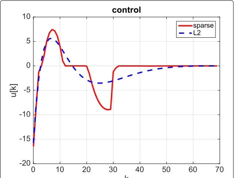
Figure 2 shows the obtained control sequenceu[k] by both MPC formulations.

Fig. 2Maximum hands-off control (solid line) andL2_{-optimal control}

(dashed line)

In this figure, the maximum hands-off control is suffi-ciently sparse (i.e., there are long time durations on which the control takes zero) while the L2-optimal control is smoother but not sparse.

The2norm of the resulting statex[k] is shown in Fig. 3. From the figure, the maximum hands-off control achieves significantly faster convergence to zero than the L2-optimal control.

Since we set the number of iterations Niter to 2 for

ADMM, there remains the difference between the exact solution, sayuˆ[k] of (8) with ξ = x[k], and the approx-imated solution, sayuADMM[k] by ADMM. To elucidate

this issue, we describe the control system with ADMM as

x[k+1]=Ax[k]+buˆ[k]+w[k] ,

w[k]b(uADMM[k]−ˆu[k]),

Fig. 3The2_{norm of the state,x[k]}

2, by maximum hands-off

where uˆ[k] and uADMM[k] are the first element of uˆ[k]

and uADMM[k], respectively. That is, the ADMM-based

control is equivalent to the exact1-optimal control with perturbationw[k], which is caused by the inexact ADMM. Figure 4 illustrates the perturbationw[k], where the exact solutionuˆ[k] is obtained by directly solving (8) byCVXin MATLABbased on the primal-dual interior point method [19]. The solution byCVXcan be taken as the exact solu-tion since the maximum relative primal-dual gap in the iteration is in this case 1.49×10−8. Figure 4 shows that the perturbation also converges to zero thanks to the stabilizing feedback mechanism (recall that, as shown in Lemma 3, the cost function is continuous, hence the feed-back loop can be expected to have favorable robustness properties.)

Finally, we compare the number of iterations between ADMM and the interior-point-basedCVX. The averaged number of the CVX iterations is 10.7, which is approx-imately five times larger than that of ADMM, Niter =

2. Note that the interior-point-based algorithm needs to solve linear equations at each iteration, and hence com-putational times may be much longer than those for the ADMM, since the inverse matrix in (13) can be computed offline.

6 Conclusions

In this paper, we have introduced the discrete-time max-imum hands-off control that maximizes the length of time duration on which the control is zero. The design is described by an0 optimization, which we have proved to be equivalent to convex 1 optimization using the restricted isometry property. The optimization can be efficiently solved by the alternating direction method of multipliers (ADMM). The extension to model predictive

Fig. 4The2norm of the perturbationw[k] by ADMM withNiter=2

control has been examined and nominal stability has been proved. Simulation results have been shown to illustrate the effectiveness of the proposed method.

6.1 Future work

Here, we show future directions related to the maximum hands-off control. The maximum hands-off control has been proposed in this paper for linear time-invariant sys-tems. It is desired to extend it to time-varying and nonlin-ear networked control, such as Markovian jump systems as discussed in [36–38], to which “intelligent methods” have been applied in [39, 40]. We believe the sparsity method can be combined with fault detection and reli-able control methods, as discussed in [41, 42]. Future work also includes an optimal selection method for the penalty parameterρin ADMM which takes into account control performance.

Endnote

1_{It is desirable if one can use an infinite-horizon control}

like anH_∞control as in e.g. [36]. However, for the maxi-mum hands-off control discussed in this paper, there is no available methods to directly obtain infinite-horizon con-trol, and model predictive control is a convenient way to extend a finite-horizon control to infinite-horizon.

Acknowledgements

The research of M. Nagahara was supported in part by JSPS KAKENHI Grant Numbers 16H01546, 15K14006, and 15H02668. The research of J. Østergaard was supported by VILLUM FONDEN Young Investigator Programme, Project No. 10095. The authors would like to thank the reviewers for pointing us to references [36–42].

Competing interests

The authors declare that they have no competing interests.

Author details

1_{Institute of Environmental Science and Technology, The University of} Kitakyushu, Hibikino, 808-0135 Fukuoka, Japan.2Department of Electronic Systems, Aalborg University, Fredrik Bajers Vej 7, B5-210, DK-9220 Aalborg, Denmark.3Department of Electrical Engineering (EIM-E), Paderborn University, Warburger Str. 100, 33098 Paderborn, Germany.

Received: 3 March 2016 Accepted: 14 June 2016

References

1. YC Eldar, G Kutyniok,Compressed Sensing: Theory and Applications. (Cambridge University Press, Cambridge, 2012)

2. T Hastie, R Tibshirani, M Wainwright,Statistical Learning with Sparsity: The Lasso and Generalizations. (CRC Press, Boca Raton, 2015)

3. K Hayashi, M Nagahara, T Tanaka, A user’s guide to compressed sensing for communications systems. IEICE Trans. Commun.E96-B(3), 685–712 (2013) 4. C Giraud,Introduction to High-Dimensional Statistics. (CRC Press, Boca

Raton, 2015)

5. I Rish, GA Cecchi, A Lozano, A Niculescu-Mizil,Practical Applications of Sparse Modeling. (MIT Press, Massachusetts, 2014)

6. H Ohlsson, F Gustafsson, L Ljung, S Boyd, in49th IEEE Conference on Decision and Control (CDC). Trajectory generation using sum-of-norms regularization, (2010), pp. 540–545

8. M Nagahara, DE Quevedo, inIFAC 18th World Congress. Sparse representations for packetized predictive networked control, (2011), pp. 84–89

9. M Nagahara, DE Quevedo, J Østergaard, Sparse packetized predictive control for networked control over erasure channels. IEEE Trans. Autom. Control.59(7), 1899–1905 (2014)

10. H Kong, GC Goodwin, MM Seron, A cost-effective sparse communication strategy for networked linear control systems: an SVD-based approach. Int. J. Robust Nonlinear Control.25(14), 2223–2240 (2015)

11. M Gallieri, JM Maciejowski, inProc. Amer. Contr. Conf.asso. MPC: Smart

regulation of over-actuated systems, (2012), pp. 1217–1222

12. M Gallieri, JM Maciejowski, inProc. 2015 European Control Conference (ECC). Model predictive control with prioritised actuators, (Linz, 2015), pp. 533–538

13. RP Aguilera, RA Delgado, D Dolz, JC Aguero, Quadratic MPC with0-input

constraint. IFAC World Congr.19(1), 10888–10893 (2014) 14. E Henriksson, DE Quevedo, EGW Peters, H Sandberg, KH Johansson,

Multiple loop self-triggered model predictive control for network scheduling and control. IEEE Trans. Control Syst. Technol.23(6), 2167–2181 (2015)

15. M Nagahara, DE Quevedo, D Neši´c, in52nd IEEE Conference on Decision and Control (CDC). Maximum hands-off control andL1_{optimality, (2013),}

pp. 3825–3830

16. M Nagahara, DE Quevedo, D Neši´c, Maximum hands-off control: a paradigm of control effort minimization. IEEE Trans. Autom. Control.

61(3), 735–747 (2016)

17. M Nagahara, DE Quevedo, D Neši´c, inSICE Control Division Multi Symposium 2014. Hands-off control as green control, (2014). http://arxiv. org/abs/1407.2377. Accessed 23 June 2016

18. T Ikeda, M Nagahara, Value function in maximum hands-off control for linear systems. Automatica.64, 190–195 (2016)

19. S Boyd, L Vandenberghe,Convex Optimization. (Cambridge University Press, Cambridge, 2004)

20. D Gabay, B Mercier, A dual algorithm for the solution of nonlinear variational problems via finite elements approximations. Comput. Math. Appl.2, 17–40 (1976)

21. S Boyd, N Parikh, E Chu, B Peleato, J Eckstein, Distributed optimization and statistical learning via the alternating direction method of multipliers. Found. Trends Mach. Learn.3(1), 1–122 (2011)

22. B O’Donoghue, G Stathopoulos, S Boyd, A splitting method for optimal control. IEEE Trans. Control Syst. Technol.21(6), 2432–2442 (2013) 23. JL Jerez, PJ Goulart, S Richter, GA Constantinides, EC Kerrigan, M Morari,

Embedded online optimization for model predictive control at megahertz rates. IEEE Trans. Autom. Control.59(12), 3238–3251 (2014) 24. AU Raghunathan, S Di Cairano, inProc. 21st International Symposium on Mathematical Theory of Networks and Systems. Optimal step-size selection in alternating direction method of multipliers for convex quadratic programs and model predictive control, (2014), pp. 807–814

25. M Annergren, A Hansson, B Wahlberg, inDecision and Control (CDC), 2012 IEEE 51st Annual Conference On. An ADMM algorithm for solving1

regularized MPC, (2012), pp. 4486–4491

26. M Grant, S Boyd, CVX: Matlab software for disciplined convex programming, version 2.1 (2014). http://cvxr.com/cvx. Accessed 23 June 2016

27. M Grant, S Boyd, inRecent Advances in Learning and Control, ed. by V Blondel, S Boyd, and H Kimura. Graph implementations for nonsmooth convex programs. Lecture Notes in Control and Information Sciences (Springer, London, 2008), pp. 95–110

28. EJ Candes, The restricted isometry property and its implications for compressed sensing. Comptes Rendus Mathematique.346(9-10), 589–592 (2008)

29. J Eckstein, DP Bertsekas, On the Douglas-Rachford splitting method and proximal point algorithm for maximal monotone operators. Math. Program.55, 293–318 (1992)

30. E Ghadimi, A Teixeira, I Shames, M Johansson, Optimal parameter selection for the alternating direction method of multipliers (ADMM): quadratic problems. IEEE Trans. Autom. Control.60(3), 644–658 (2015) 31. BS He, H Yang, SL Wang, Alternating direction method with self-adaptive

penalty parameters for monotone variational inequalities. J. Optim. Theory Appl.106(2), 337–356 (2000)

32. SL Wang, LZ Liao, Decomposition method with a variable parameter for a class of monotone variational inequality problems. J. Optim. Theory Appl.

109(2), 415–429 (2001)

33. JM Maciejowski,Predictive Control with Constraints. (Prentice-Hall, Essex, 2002)

34. JB Rawlings, DQ Mayne,Model Predictive Control Theory and Design. (Nob Hill Publishing, Madison, 2009)

35. L Grüne, J Pannek,Nonlinear Model Predictive Control. (Springer, London, 2011)

36. Y Wei, J Qiu, S Fu, Mode-dependent nonrational output feedback control for continuous-time semi-Markovian jump systems with time-varying delay. Nonlinear Anal. Hybrid Syst.16, 52–71 (2015)

37. Y Wei, J Qiu, HR Karimi, M Wang,H∞model reduction for

continuous-time Markovian jump systems with incomplete statistics of mode information. Int. J. Syst. Sci.45(7), 1496–1507 (2014)

38. Y Wei, J Qiu, HR Karimi, M Wang, Filtering design for two-dimensional Markovian jump systems with state-delays and deficient mode information. Inf. Sci.269, 316–331 (2014)

39. T Wang, Y Zhang, J Qiu, H Gao, Adaptive fuzzy backstepping control for a class of nonlinear systems with sampled and delayed measurements. IEEE Trans. Fuzzy Syst.23(2), 302–312 (2015)

40. T Wang, H Gao, J Qiu, A combined adaptive neural network and nonlinear model predictive control for multirate networked industrial process control. IEEE Trans. Neural Netw. Learn. Syst.27(2), 416–425 (2016) 41. L Li, SX Ding, J Qiu, Y Yang, Y Zhang, Weighted fuzzy observer-based fault

detection approach for discrete-time nonlinear systems via piecewise-fuzzy Lyapunov functions. IEEE Trans. Fuzzy Syst. (2016) 42. J Qiu, SX Ding, H Gao, S Yin, Fuzzy-model-based reliable static output

feedbackH∞control of nonlinear hyperbolic PDE systems. IEEE Trans. Fuzzy Syst.24(2), 388–400 (2016)

Submit your manuscript to a

journal and benefi t from:

7Convenient online submission

7Rigorous peer review

7Immediate publication on acceptance

7Open access: articles freely available online

7High visibility within the fi eld

7Retaining the copyright to your article