R E S E A R C H
Open Access
Effect of embedded unbiasedness on
discrete-time optimal FIR filtering estimates
Shunyi Zhao
1, Yuriy S. Shmaliy
2*, Fei Liu
1, Oscar Ibarra-Manzano
2and Sanowar H. Khan
3Abstract
Unbiased estimation is an efficient alternative to optimal estimation when the noise statistics are not fully known and/or the model undergoes temporary uncertainties. In this paper, we investigate the effect of embedded
unbiasedness (EU) on optimal finite impulse response (OFIR) filtering estimates of linear discrete time-invariant state-space models. A new OFIR-EU filter is derived by minimizing the mean square error (MSE) subject to the unbiasedness constraint. We show that the OFIR-UE filter is equivalent to the minimum variance unbiased FIR (UFIR) filter. Unlike the OFIR filter, the OFIR-EU filter does not require the initial conditions. In terms of accuracy, the OFIR-EU filter occupies an intermediate place between the UFIR and OFIR filters. Contrary to the UFIR filter which MSE is minimized by the optimal horizon ofNoptpoints, the MSEs in the OFIR-EU and OFIR filters diminish withNand these filters are thus
full-horizon. Based upon several examples, we show that the OFIR-UE filter has higher immunity against errors in the noise statistics and better robustness against temporary model uncertainties than the OFIR and Kalman filters.
Keywords: State estimation; Unbiased FIR filter; Optimal FIR filter; Kalman filter
1 Introduction
Beginning with the works by Gauss [1], unbiasedness plays a role of the necessary condition that is used to derive linear and nonlinear estimators [2]. In statistics and sig-nal processing, the ordinary least squares (OLS) estimator proposed by Gauss in 1795 is an unbiased estimator. By the Gauss-Markov theorem [3], this estimator is also the best linear unbiased estimator (BLUE) [4] if noise is white and if it has the same variance at each time step [5]. The unbiasedness is obeyed by a condition E{ˆxk} = E{xk} which means that the average of estimatexˆk is equal to that of the modelxk. It leads to the unbiased finite impulse response (UFIR) estimator [6]. Of practical importance is that neither OLS nor UFIR require the noise statis-tics which are not always known to the engineers [7]. The unbiasedness condition, however, does not guarantee “good estimate” [8]. Therefore, the sufficient condition— minimized noise variance—is often applied along to pro-duce different kinds of estimators which are optimal in the minimum mean square error (MSE) sense or subop-timal: Bayesian, maximum likelihood (MLE), minimum
*Correspondence: [email protected]
2Department of Electronics Engineering, Universidad de Guanajuato, Salamanca 36885, Mexico
Full list of author information is available at the end of the article
variance unbiased (MVU), etc. In recent decades, a new class of estimators having FIR (filters, smoothers, and pre-dictors) was developed to have optimal or suboptimal properties.
The FIR filter utilizes finite measurements over the most recent time interval (horizon) ofNdiscrete points. Compared to the filters with infinite impulse response (IIR), such as the Kalman filter (KF) [9], the FIR fil-ter exhibits some useful engineering features such as the bounded input/bounded output (BIBO) stability [10], robustness against temporary model uncertainties and round-off errors [11], and lower sensitivity to noise [12]. The most noticeable early works on optimal FIR (OFIR) filtering are [13–15]. At that time, FIR filters were not the ones commonly used for state estimation due to the ana-lytical complexity and large computational burden. Nowa-days, the interest to FIR estimators has grown owing to the tremendous progress in the computational resources. Accordingly, we find a number of new solutions on FIR filtering [16–21], smoothing [22–24], and prediction [25–27] as well as efficient applications [28–30].
Basically, the unbiasedness can be satisfied in two dif-ferent strategies: (1) one may test an estimator by the
unbiasedness condition or (2) one may embed the unbi-asedness constraint into the design. We therefore recog-nize below the checked (tested) unbiasedness (CU) and the embedded unbiasedness (EU). Accordingly, we denote the FIR filter with CU as FIR-CU and the FIR filter with EU as FIR-EU.
In state estimation, signal processing, tracking, and con-trol, two different state-space models are commonly used. The prediction model which is basic in control isxk+1 = Axk+Bwkandyk =Cxk+Dvk, in whichwkandvkare noise vectors, and A,B,C andDare relevant matrices. Employing this model, the receding horizon FIR estima-tors were proposed for different types of unbiasedness. In [16], the receding horizon FIR-CU filter was derived from KF with no requirements for the initial state. Soon after, a receding horizon FIR-EU filter was proposed by Kwon, Kim, and Han in [17], where the unbiasedness condition was considered as a constraint to the optimiza-tion problem. Later, the receding horizon FIR smoothers were found in [22] for CU by employing the maximum likelihood and in [24] for EU by minimizing the error variance.
The real-time state modelxk = Axk−1+Bwk is used in signal processing when the prediction is not required (different time index) [31, 32]. Employing this model, the FIR-CU filter and smoother were proposed by Shmaliy in [23, 33] for polynomial systems. In [12], a p-shift unbi-ased FIR filter (UFIR) was derived as a special case of the OFIR filter. Here, the unbiasedness was checked a pos-teriori, and the solution thus belongs to CU. Soon after, the UFIR filter [12] was extended to time-variant systems [18, 34]. For nonlinear models, an extended UFIR filter was proposed in [35] and unified forms for FIR filter-ing and smoothfilter-ing were discussed in [36]. An important advantage of the UFIR filter against OFIR filter is that the noise statistics are not required. Because noise reduction in FIR structures is provided by averaging,N 1 makes the UFIR filter as successful in accuracy as the OFIR filter. It has to be remarked now that all of the aforemen-tioned FIR estimators related to real-time state-space model belong to the CU solutions. Still no optimal FIR estimator was addresses of the EU type. It is thus unclear which kind of FIR estimators serves better in particular applications [37–39]. So, there is still room for discussion of the best FIR filter.
In this paper, we systematically investigate effect of the embedded unbiasedness on OFIR estimates. To this end, we derive a new FIR filter, called OFIR-EU filter, by min-imizing the MSE subject to the unbiasedness constraint. We also learn properties of the OFIR-EU filter in a com-parison with the OFIR and UFIR filters and KF. The remaining part of the paper is organized as follows. In Section 2, we describe the model and formulate the prob-lem. The OFIR-EU filter is derived in Section 3. Here, we
also consider a unified form for different kinds of OFIR filters. In Section 4, we generalize several FIR filters and discuss special cases of the OFIR-EU filter. The MSEs are compared analytically in Section 5. Extensive simulations are provided in Section 6, and concluding remarks are drawn in Section 7.
The following notations are used: Rn denotes the n -dimensional Euclidean space; E{·} denotes the expected value; diag(e1· · ·em) represents a diagonal matrix with
diagonal elementse1,· · ·,em; trMis the trace ofM; andI is the identity matrix of proper dimensions.
2 Preliminaries and problem formulation
Consider a linear discrete-time model given with the state-space equations
xk = Axk−1+Bwk, (1) yk = Cxk+Dvk, (2)
in whichkis the discrete time index,xk ∈Rnis the state vector, andyk ∈ Rpis the measurement vector. Matrices A∈Rn×n,B∈Rn×u,C∈Rp×nandD∈Rp×vare time-invariant and known. We suppose that the process noise
wk ∈ Ru and the measurement noisevk ∈ Rv are zero mean,E{wk} =0andE{vk} = 0, mutually uncorrelated, and have arbitrary distributions and known covariances
Q(i,j) = EwiwTj
,R(i,j) = EvivTj
for alliandj, to mean thatwkandvkare not obligatorily white Gaussian.
Following [12], the state-space model (1) and (2) can be represented in a batch form on a discrete time inter-val [l,k] with recursively computed forward-in-time solu-tions as
Xk,l = Ak−lxl+Bk−lWk,l, (3) Yk,l = Ck−lxl+Hk−lWk,l+Dk−lVk,l, (4)
where l = k − N + 1 is a start point of the
averag-ing horizon. The time-variant state vectorXk,l ∈ RNn×1, observation vector Yk,l ∈ RNp×1, process noise vector Wk,l∈RNu×1, and observation noise vectorVk,l∈RNv×1 are specified as, respectively,
Xk,l =
xTk xTk−1· · ·xTl
T
, (5)
Yk,l =
yTk yTk−1· · ·yTl
T
, (6)
Wk,l =
wTk wTk−1· · ·wTl T, (7)
Vk,l =
vTk vTk−1· · ·vTl
T
. (8)
The extended model matrix Ak−l ∈ RNn×n,
measurement noise matrixDk−l ∈ RNp×Nv are all
time-invariant and dependent on the horizon length of N
points. Model (1) and (2) suggests that these matrices can be written as, respectively,
Note that at the start horizon point we have an equation
xl =xl+Bwlwhich is satisfied uniquely with zero-valued wl, provided thatBis not zeroth. The initial statexlmust thus be known in advance or estimated optimally.
The FIR filter applied toN past neighboring measure-ment points on a horizon [l,k] can be specified with
ˆ
xk|k=KkYk,l, (15) wherexˆk|k is the estimate1, andKk is the FIR filter gain determined using a given cost criterion. Note that a dis-tinctive difference between the FIR with IIR filters is that only one nearest past measurement is used in the recur-sive IIR (Kalman) filter to provide the estimate, while the convolution-based batch FIR filter requiresNmost recent measurements.
The estimate (15) will be unbiased if to obey the follow-ing unbiasedness condition,
E{xk} =E{ˆxk|k}, (16)
in whichxkcan be specified as
xk=AN−1xl+ ¯Bk−lWk,l (17)
if to combine (3) and (4). HereB¯k−lis the first vector row inBk−l. By substituting (15) and (17) into (16), replacing the termYk,l with (4), and providing the averaging, one arrives at the unbiasedness constraint
AN−1=KkCk−l (18)
which is also known as the deadbeat constraint [19]. Pro-videdxˆk|k, the instantaneous estimation error ek can be defined as
ek =xk− ˆxk|k. (19)
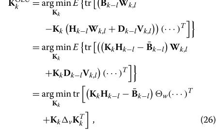
The problem now formulates as follows. Given the mod-els, (1) and (2), we would like to derive an OFIR-EU filter by minimizing the variance of the estimation error (19) as
KOEUk = arg min
Kk
EekeTk
subject to(18). (20)
We also wish to investigate effect of the unbiasedness constraint (18) on the OFIR-EU estimate, compare errors in different kinds of FIR filters, and analyze the trade-off between the OFIR-EU filter derived in this paper, UFIR filter [33], OFIR filter [34], and KF under the diverse operation conditions.
3 OFIR-EU filter
In the derivation of the OFIR-EU filter, the following lemma will be used.
Lemma 1.The trace optimization problem is given by
arg min the trace ofM,θ denotes the constraint indication param-eter such thatθ = 1 if the constraint exists andθ = 0 otherwise. Here,F,G,H,L,M,P,S,U, andZare constant matrices of appropriate dimensions. The solution to (21) is
K=
Proof.The proof is provided in Appendix A.
3.1 The gain for OFIR-EU filter
subject to (18), where(· · ·)denotes the term that is equal to the relevant preceding term. By substituting xk with (17) andxˆk|kwith (15), the cost function becomes
If to take into account constraint (18), provide the aver-aging, and rearrange the terms, (25) can be transformed to
where the fact is invoked that the system noise vector
Wk,land the measurement noise vectorVk,lare pairwise independent. The auxiliary matrices are
w=E
Referring to Lemma 1 withθ = 1, the solution to the optimization problem (26) can be obtained by neglecting
L,M, andPand using the replacements:F←Hk−l,G← The OFIR-EU filter structure can now be summarized in the following theorem.
Theorem 1.Given the discrete time-invariant state space model (1) and (2) with zero mean mutually inde-pendent and uncorrelated noise vectors wk and vk, the
OFIR-EU filter utilizing measurements from l to k is stated by
ˆ
xk|k =KOEUk Yk,l, (35)
whereKOEUk =KOEUak +KkOEUb,Yk,l ∈RNp×1is the mea-surement vector given by (6), andKOEUak andKOEUbk are given by (30) and (31) withCk−landB¯k−lspecified by (11) and the first row vector of (10), respectively.
Proof. The proof is provided by (24)-(34).
Note that the horizon lengthN for (35) should be cho-sen such that the first inverse in (30) exists. In general,
N can be set asN n, where n is the number of the
model states. Table 1 summarizes the steps in the OFIR-EU estimation algorithm, in which the noise statistics are
assumed to be known for measurements available froml
tok.
GivenN, computeKOEUak andKOEUbk according to (30) and (31), respectively, then the OFIR-EU estimate can be obtained at time indexkby (35).
3.2 Unified form for OFIR and OFIR-EU filters
In order to ascertain a correspondence between the OFIR filter and its modifications associated with the unbiased-ness constraint (18), we rewrite the optimization problem (24) regarding the unified gainKUOk as
KUOk =arg min
is the mean square of initial statexl. Using Lemma 1 and substituting
F←Hk−l,G← ¯Bk−l,H←w,P←x,S←v,
M=Z←AN−1,L=U←Ck−l,
we find a solution to (36) as
KUOk =θAN−1k−l
Table 1The OFIR-EU filtering Algorithm
Stage
Given: Nn, l=k−N+1
Find: KOEUak by (30) andKOEUbk by (31)
Compute: xˆk|k=(KOEUa
where into consideration that the second term on the right-hand side of (42) equals to zero, we come up with a deduction that
KUOk =KOEUk . (43)
In the unconstrained case ofθ =0, (37) transforms to
KUOk =AN−1xCTk−l−x+1w+v
+ ¯Bk−lwHTk−l−x+1w+v. (44)
By multiplyingx with identity
CTk−lCk−l
−1
CTk−lCk−l from the left-hand side, (44) turns up as
KUOk =
where the unbiased gainKUk is defined by [6]
KUk =AN−1
CTk−lCk−l
−1
CTk−l. (46)
We thus infer that this case corresponds to the OFIR fil-ter which gain was found in [34]. At this point, we notice that (37) is a unified generalized form for the OFIR filter gain which minimize the MSE in the estimate of discrete time-invariant state-space model. In this regard, the OFIR filter gain derived in [34] and OFIR-EU filter gain spec-ified by Theorem 1 can be considered as special cases of (37).
4 MVU FIR filter
Owing to its unique properties, the unbiasedness con-straint (18) has been employed extensively to derive dif-ferent kinds of FIR filters [6, 15–17, 23]. The UFIR filter was shown in [12] to be a special case of the OFIR filter with the unbiased gain specified by (46), whereNis cho-sen asN nto guarantee the invertibility ofCTk−lCk−l. The gain (46) can also be obtained by multiplyingAN−1in
the constrain (18) from the right-hand side with the
iden-tity matrix CTk−lCk−l
−1
CTk−lCk−l and neglecting Ck−l in both sides. In this sense, the UFIR filter is akin to Gauss’s OLS. On the other hand, (46) does not guarantee optimality in the MSE sense. An optimized solution can be provided by minimizing the error variance that leads to the minimum variance unbiased (MVU) FIR filter [40]. Since the properties of the MVU FIR filter are in-between the UFIR and OFIR filters, a unified form for the UFIR fil-ter can also be assumed. Below, we specify the MVU FIR filter and show a unified relationship between the UFIR, MVU FIR, and OFIR-EU filter gains.
4.1 Identity of MVU FIR and OFIR-EU filters
It has been shown in [40] that the variance can be min-imized in the UFIR filter if to represent the gain of the MVU FIR filterKMVUk as a linear combination ofKUk given by (46) and an auxiliary termKakof the same class,
KMVUk =KUk +Kak, (47)
On the other hand, Lemma 1 suggests thatKMVUk does not depend on the initial state matrix x. Any x can thus be supposed in (50), provided that the inverse in (50) exists. This fundamental property was postulated in many papers [11, 17, 23, 33] and, based upon, KMVUk can be some rearrangements, we arrive at an aquality
KMVUk =KUk −KUk I−k−l
Theorem 2.The MVU FIR filter specified by (47) is identical to the OFIR-EU filter specified by Theorem 1,
KMVUk =KOEUk .
Proof. The proof is given in Section 4.1.
It follows from Theorem 2 that the gainKMVUk is not unique. One may suppose any initial state matrixx, com-pute it by solving the discrete algebraic Riccati equation
(DARE) as in [12], or even neglect x as we have done
above. Although each of these cases require particular algorithms, Lemma 1 suggests that the estimation
accu-racy will not be affected by x. We notice that this
property of MVU FIR filter was unknown so far. We use it below while comparing different kinds of unbiased FIR filters.
4.2 Unified form for UFIR and MVU FIR filters
The basic UFIR filter gain found in [12] is given by (46). There can be found other forms of this gain if to multi-plyAN−1in the constraint (18) from the right-hand side with an appropriate identity matrix and removeCk−lfrom the both sides. The unbiased gainKUUk produced in such a way depends on an auxiliary matrixZk−l, provided that its inverse exists. However, a class of UFIR filters asso-ciated withZk−lmust have some reasonable formulation which can be the following. Let us combineKUUk with two additive components of the same class as
KUUk =KUUak +κKUUbk , (55) cial cases can be recognized:
– Ifκ =0andk−l=λIwithλconstant, then KUUk =KUk .
– Ifκ =1andk−l=−w+1v, thenKUUk =KOEUk .
Several other generalizations can also be made regard-ing the types of systems:
4.2.1 Deterministic state model
If the state model (1) is noiseless, then the term containing
wshould be omitted in (30) and (31), and (29) reduces to the gain
v . This gain corresponds to the traditional BLUE and MLE for Gaussian models [5]. The batch form (59) was also shown in [11] for the receding horizon FIR filter with embedded unbiasedness and minimized variance.
4.2.2 Deterministic measurement model
If the observation model (2) is noise-free, one has
KOEUk =AN−1
Having no noise in (1) and (2), the cost function in (25) becomes
By the constraint (18), the terms in the parentheses of (61) become identically zero. Hence, the solution to (61) is the unbiased gainKkgiven by (46). It then follows that
The UFIR filter is a deadbeat filter for deterministic systems.
If (18) is not applied, then the solution to (61) becomes
KOk =AN−1xCTk−l−x1. (62) left-hand side in (62) yields
KOk =KUk =AN−1
CTk−lCk−l
−1
CTk−l (63)
which can also be obtained by setting the termswand
vin (45) to zero. We thus infer that
The OFIR filter is a deadbeat filter for deterministic systems.
Table 2 summarizes the gains for the UFIR, OFIR-EU (MVU FIR), and OFIR filters. Note that all these filter gains are given in the batch form, where the computa-tional complexity is large when the estimation horizon is long. Therefore, corresponding iterative realization is required for a fast computation.
Table 2Different FIR filter gains
5 Estimation errors
Provided a correspondence between the OFIR, OFIR-EU (MVU FIR), and UFIR filter gains (Table 2), in this section, we proceed with an analysis of the estimation errors. We compare the MSEs of these filters and point out their common features and differences.
5.1 Mean square errors
The MSEJkat the estimator output can be defined as
Jk=E{ekek} =E
where each of the mean square values can be decom-posed via the squared bias and variance. Assuming that the actualxk is inherently unbiased, we writeE{xkxTk} =
and finally transforme (64) to
Jk=Bias2
where the state variance Var(xk)is specified by
Var(xk)= ¯Bk−lwB¯Tk−l (66)
and, for unbiased estimate, we have
Biasxˆk|k
=0. (67)
Based upon (65), below we specify the MSEs for the above considered FIR filters.
5.1.1 MSE in the UFIR estimate
For the UFIR filter, the third term Var(xˆk|k)on the right-hand side of (65) can be transformed to
Var(xˆk|k)=E Accordingly, the MSE in the UFIR filter becomes
JUk = ¯Bk−lwB¯Tk−l+KUkw+v
whereKUk is given by (46). The MSE (70) was first studied in [18].
5.1.2 MSE in the OFIR-EU estimate
For the OFIR-EU filter, Var(xˆk|k) and Cov(xk,xˆk|k) are
Next, substituting (66), (73) and (74) into (65) and rear-ranging the terms yield
Finally, by invoking ϒk−l given by (53), we transform (75) to
5.1.3 MSE in the OFIR estimate
We first notice that the OFIR filter gainKOk given by (45) can equivalently be rewritten as
KOk =KUk (x+w+v−w+v) −x+1w+v + ¯Bk−lwHTk−l−x+1w+v
=KUk + ¯ϒk−l. (77)
For this filter, the bias-dependent term becomes
Bias2xˆk|k
= ¯ϒk−lxϒ¯kT−l. (78) Now, by combining (65), (68), and (69), the MSE of the OFIR filter can be found to be
JOk = ¯ϒk−lxϒ¯kT−l+ ¯Bk−lwB¯Tk−l
JOk =JUk − ¯ϒk−lx+w+vϒ¯kT−l. (80)
The above-provided relations (70), (76), and (80) allow analyzing effect of the unbiasedness constraint on the OFIR-filtering estimates that we provide below.
5.2 Correspondence between the MSEs
A general relationship between the MSEs associated with different FIR filters is ascertained by the following theorem.
Theorem 3. Given the MSEsJUk,JOEUk andJOk, defined by (70), (76) and (80), respectively, then the following inequal-ity holds,
JOk JOEUk JUk , (81)
and it becomes an equality when the state-space model is deterministic.
Proof. The proof is given in [40] and we support it with a simple analysis. The UFIR filter is designed to obtain zero bias. Although the noise variance is reduced here as
∝ 1
N, the optimality is not guaranteed. Therefore, the MSE in UFIR filter generally exceeds those in two other filters. The MSE in the OFIR filter is minimal among other filters. The OFIR-EU filter minimizes MSE with the embedded unbiasedness. Its error is thus in between the UFIR and OFIR filters.
6 Applications
Theorem 3 states that the OFIR-EU and MVU FIR fil-ters produce intermediate estimates between the OFIR and UFIR filters. In order to learn the effect of the embedded unbiasedness in more detail, we test the UFIR, OFIR-EU, and OFIR filters in line with the KF in differ-ent noise environmdiffer-ents by a two-state polynomial model specified with
A=
1 0.05
0 1
.
The reader can also find some other comparisons of the KF and FIR filters in [16, 18, 34, 41].
6.0.1 Accurate model—ideal case
In an ideal case, one may think that the model represents a process accurately and the noise statistics are known exactly. The goal then is to learn the effect of the horizon
lengthN on the FIR estimates. We set the measurement
noise variance asσv2=10, and the initial states asx10=1
andx20=0.01 /s.
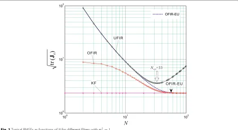
We then compute the root MSE (RMSE) of the estimate by trJk as a function ofN. The results are illustrated in Fig. 1 for σw2 = 1 and in Fig. 2 forσw2 = 0.1. What we
can see here is that the MSE function of the UFIR filter is traditionally concave onNwith a minimum atNopt[42]:
withN < Nopt, noise reduction is inefficient and, ifN >
Nopt, the bias error dominates. On the other hand, the KF
isN-invariant and its MSE is thus constant. The following generalizations can also be made:
– The embedded unbiasedness puts the OFIR-EU filter error in between the UFIR and OFIR filters: the OFIR-EU filter becomes essentially the UFIR filter whenN<Noptand theOFIR filter ifN>Nopt.
– The OFIR and OFIR-EU estimates converge to the KF estimate by increasing the averaging horizonN. The estimates become practically indistinguishable whenNNopt.
– An increase inNoptdiminishes the error difference
between the OFIR and UFIR filters (compare Fig. 1 withNopt=33and Fig. 2 withNopt=47).
– Because the MSEs in theOFIR and OFIR-EU filters diminish withN, these filters are full-horizon [18].
6.0.2 Filtering with errors in the noise statistics
The noise statistics required by the KF are commonly not completely know to the engineer. In order to investigate the effect of the imprecisely defined noise covariances in the worst case, we introduce a correction coefficientpas p2QandR/p2, varypfrom 0.1 to 10, and plot the RMSE √
trJkas shown in Fig. 3.
Note that the MSE functions of optimal filters are inher-ently concave onpwith a minimum atp=1 and the MSE of the UFIR filter isp-invariant.
As expected,p=1 makes the OFIR filter, OFIR-EU fil-ter, and KF a bit more accurate than the UFIR filter. But, that is only within a narrow range of p(0.6 < p < 1.5 in Fig. 3) that the KF slightly outperforms the UFIR filter. Otherwise, the UFIR filter demonstrates smaller errors. Referring to practical difficulties in the determination of noise statistics [7], the latter can be considered as an important engineering advantage of the UFIR filter. Some other generalizations also emerge from Fig. 3:
– The embedded unbiasedness makes the OFIR-EU filterp-invariant withp<1. In this sense, the OFIR-EU is equal here to the UFIR filter, and this can be considered as a particular meaningful property of the approach proposed.
– Withp<1, the KF is more sensitive to errors in the noise statistics than the FIR filters.
– Byp>1, the MSEs in the KF, OFIR filter, and OFIR-EU filter grow and converge.
Fig. 1Typical RMSEs as functions ofNfor different filters withσw2=1
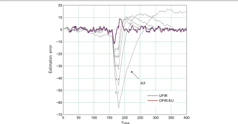
6.0.3 Filtering with model uncertainties
To learn effect of the temporary model uncertainties on the filtering accuracy, in this section we setτ =0.1 s when
160k180 andτ =0.05 s otherwise. The noise
vari-ances are allowed to beσw21=1,σw22=1/s2, andσv2=10. The process is simulated at 400 subsequent points.
Typical filtering estimates are sketched in Fig. 4. As can be seen, the OFIR-EU filter (case p = 0.2) and the UFIR filter produce almost equal errors and demonstrate good robustness against the uncertainties. Just on the con-trary, the KF demonstrates much worse robustness for any
p1.
Fig. 3Typical RMSE√trJkas a function ofpfor KF and FIR filters
7 Conclusions
Summarizing, we notice that the unbiasedness imbedded to the OFIR filter instills into it several useful prop-erties. Unlike the OFIR filter, the OFIR-EU filter com-pletely ignores the initial conditions. The OFIR-EU filter
is equivalent to the MVU FIR filter. In terms of accuracy, the OFIR-EU filter is in between the UFIR and OFIR fil-ters. Unlike in the UFIR filter which MSE is minimized by Nopt, MSEs in the OFIR-EU and OFIR filters
dimin-ish with N and these filters are thus full-horizon. The
performance of OFIR-EU filter is developed by varying
the horizon N around Nopt or ranging the correction
coefficient paround p = 1. Accordingly, the OFIR-EU
filter in general demonstrates higher immunity against errors in the noise statistics and better robustness against temporary model uncertainties than the OFIR filter and KF.
Referring to the fact that optimal FIR filters are essen-tially the full-horizon filters but their batch forms are computationally inefficient, we now focus our attention on the fast iterative form for OFIR-EU filter and plan to report the results in near future.
Endnote 1xˆ
k|kmeans the estimate atkvia measurements from the past tok.
Appendix A: Proof of Lemma 1
Represent the performance criterion in (21) as
φ=tr
(KF−G)H(KF−G)T+(KL−M)P
×(KL−M)T+KSKT. (82)
By partitioningKasKT =[k1k2· · ·km], wheremis the dimension ofK, rewriteφas
φ = lines, theith constraint can be specified by
Li{
reduced tomindependent optimization problems as
min
whereλidenotes theith vector of the Lagrange multiplier. Note thatϕi|θ depends onθ which governs the existing of constraint. Settingθ = 1, first consider a general case of
F = U,L= U,G = ZandM =Zwhich is denoted as
case (a). Taking the derivative ofϕi|awith respect tokiand
λirespectively and making them equal to zero lead to
∂ϕi|a
∂ki|a =
2aki|a−2(FHgi+LPmi)+Uλi=0 , (88)
which can further be rewritten as
ki|a=−a1 By multiplying the both sides of (89) with UT from the left-hand side, using the constraint (85), and arranging the terms, arrive at
Substituting (90) into (89) and taking into account that
H=HT,P=PT,S=STanda=Ta, transformskTi to
At this point, reconstructKaas
Ka= as case (c), the solutions can be obtained similarly to case (a), respectively,
In the case ofθ = 0 which is denoted as case (d), the
whereis specified by (23). An equivalent form of (100) is (22) and the proof is complete.
Competing interests
The authors declare that they have no competing interests.
Acknowledgements
This investigation was supported by the Royal Academy of Engineering under the Newton Research Collaboration Programme NRCP/1415/140.
Author details
1Key Laboratory of Advanced Process Control for Light Industry (Ministry of
Education), Institute of Automation, Jiangnan University, Wuxi 214122, P.R. China.2Department of Electronics Engineering, Universidad de Guanajuato, Salamanca 36885, Mexico.3School of Mathematics, Computer Science and
Engineering, City University of London, London EC1V 0HB, UK.
Received: 29 April 2015 Accepted: 21 August 2015
References
1. CF Gauss,Theory of the combination of observations least subject to errors.
(SIAM Publ, Philadelphia, 1995). Transl. by Stewart GW
2. H Stark, JW Woods,Probability, random processes, and estimation theory for engineers, 2nd edn. (Prentice Hall, Upper Saddle River, NJ, 1994) 3. JH Stapleton,Linear statistical models, 2nd edn. (Wiley, New York, 2009) 4. AC Aitken, On least squares and linear combinations of observations.
Proc. R. Soc. Edinb.55, 42–48 (1935)
5. SM Kay,Fundamentals of statistical signal processing. (Prentice Hall, New York, 2001)
6. YS Shmaliy, An unbiased FIR filter for TIE model of a local clock in applications to GPS-based timekeeping. IEEE Trans. Ultrason. Ferroelec. Freq. Control.53(5), 862–870 (2006)
7. BP Gibbs,Advanced Kalman filtering, least-squares and modeling. (John Wiley & Sons, Hoboken, NJ, 2011)
8. M Hardy, An illuminating counterexample. Am. Math. Mon.110(3), 232–238 (2003)
9. D Simon,Optimal state estimation: Kalman, Hinf, and nonlinear approaches. (John Wiley & Sons, Honboken, NJ, 2006)
10. AH Jazwinski,Stochastic processes and filtering theory. (Academic, New York, 1970)
11. WH Kwon, S Han,Receding horizon control: model predictive control for state models. (Springer, London, 2005)
12. YS Shmaliy, Linear optimal FIR estimation of discrete time-invariant state-space models. IEEE Trans. Signal Process.58(6), 3086–2010 (2010) 13. KR Johnson, Optimum, linear, discrete filtering of signals containing a
nonrandom component. IRE Trans. Inf. Theory.2(2), 49–55 (1956) 14. AH Jazwinski, Limited memory optimal filtering. IEEE Trans. Autom. Contr.
13(10), 558–563 (1968)
15. CK Ahn, S Han, WH Kwon, FIR filters for linear continuous-time state-space systems. IEEE Signal Process. Lett.13(9), 557–560 (2006)
16. WH Kwon, PS Kim, P Park, A receding horizon Kalman FIR filter for discrete time-invariant systems. IEEE Trans. Autom. Contr.99(9), 1787–1791 (1999) 17. WH Kwon, PS Kim, S Han, A receding horizon unbiased FIR filter for
discrete-time state space models. Automatica.38(3), 545–551 (2002) 18. YS Shmaliy, An iterative Kalman-like algorithm ignoring noise and initial
conditions. IEEE Trans. Signal Process.59(6), 2465–2473 (2011) 19. YS Shmaliy, Optimal gains of FIR estimations for a class of discrete-time
state-space models. IEEE Signal Process. Lett.15, 517–520 (2008) 20. CK Ahn, Strictly passive FIR filtering for state-space models with external
disturbance. Int. J. Electron. Commun.66(11), 944–948 (2012) 21. JM Park, CK Ahn, MT Lim, MK Song, Horizon group shift FIR filter:
alternative nonlinear filter using finite recent measurement. Measurement.57, 33–45 (2014)
22. CK Ahn, PS Kim, Fixed-lag maximum likelihood FIR smoother for state-space modelsIEICE Electron. IEICE Electron. Express.5(1), 11–16 (2008)
23. YS Shmaliy, LJ Morales-Mendoza, FIR Smoothing of discrete-time polynomial signals in state space. IEEE Trans. Signal Process.58(5), 2544–2555 (2010)
24. BK Kwon, S Han, OK Kim, WH Kwon, Minimum variance FIR smoothers for discrete-time state space models. EEE Trans. Signal Process. Lett.14(8), 557–560 (2007)
25. L Danyang, L Xuanhuang, Optimal state estimation without the requirement of a prior statistics informantion of the initial state. IEEE Trans. Autom. Contr.39(10), 2087–2091 (1994)
26. KV Ling, KW Lim, Receding horizon recursive state estimation. IEEE Trans. Autom. Contr.44(9), 1750–1753 (1999)
27. J Makhoul, Linear prediction: a tutorial review. Proc. IEEE.63, 561–580 (1975)
28. J Levine, The statistical modeling of atomic clocks and the design of time scales. Rev. Sci. Instrum.83, 021101-1–021101-28 (2012)
29. Y Kou, Y Jiao, D Xu, M Zhang, Ya Liu, X Li, Low-cost precise measurement of oscillator frequency instability based on GNSS carrier observation. Adv. Space Res.51(6), 969–977 (2013)
30. JW Choi, S Han, JM Cioffi, An FIR channel estimation filter with robustness to channel mismatch condition. IEEE Trans. Broadcast.54(1), 127–130 (2008)
31. J Salmi, A Richter, V Koivunen, Detection and tracking of MIMO propagation path parameters using state-space approach. IEEE Trans. Signal Process.57(4), 1538–1550 (2009)
32. I Nevat, J Yuan, Joint channel tracking and decoding for BICM-OFDM systems using consistency test and adaptive detection selection. IEEE Trans. Veh. Technol.58(8), 4316–4328 (2009)
33. YS Shmaliy, Unbiased FIR filtering of discrete-time polynomial state-space models. IEEE Trans. Signal Process.57(4), 1241–1249 (2009)
34. YS Shmaliy, O Ibarra-Manzano, Time-variant linear optimal finite impulse response estimator for discrete state-space models. Int. J. Adapt. Contrl Signal Process.26(2), 95–104 (2012)
35. YS Shmaliy, Suboptimal FIR filtering of nonlinear models in additive white Gaussian noise. IEEE Trans. Signal Process.60(10), 5519–5527 (2012) 36. D Simon, YS Shmaliy, Unified forms for Kalman and finite impulse
37. YL Wei, J Qiu, HR Karimi, M Wang, A new design ofH∞filtering for continuous-time Markovian jump systems with time-varying delay and partially accessible mode information. Signal Process.93(9), 2392–2407 (2013)
38. YL Wei, M Wang, J Qiu, New approach to delay-dependentHαfiltering for discrete-time Markovian jump systems with time-varying delay and incomplete transtion descriptions. IET Control Theory Appl.7(5), 684–696 (2013)
39. J Qiu, YL Wei, HR Karimi, New approach to delay-dependentHαcontrol for continuous-time Markovian jump systems with time-varying delay and deficient transtion descriptions. J. Frankl. Inst.352(1), 189–215 (2015) 40. S Zhao, YS Shmaliy, B Huang, F Liu, Minimum variance unbiased FIR filter
for discrete time-variant models. Automatica.53, 355–361 (2015) 41. PS Kim, An alternative FIR filter for state estimation in discrete-time
systems. Digit. Signal Process.20(3), 935–943 (2010)
42. FR Echeverria, A Sarr, YS Shmaliy, Optimal memory for discrete-time FIR filters in state-space. IEEE Trans. Signal Process.62, 557–561 (2014)
Submit your manuscript to a
journal and benefi t from:
7Convenient online submission
7Rigorous peer review
7Immediate publication on acceptance
7Open access: articles freely available online
7High visibility within the fi eld
7Retaining the copyright to your article