Computational Intelligence Algorithms for Optimisation of Wireless Sensor Networks

Algorithms for Optimisation of

Wireless Sensor Networks

A thesis submitted in partial fulfilment of the requirements for the

Degree of Doctor of Philosophy

BY

Muyiwa Olakanmi Oladimeji

Student ID 3023261

Supervised by

Dr Sandra Dudley

School of Engineering, London South Bank University

adult years, for encouraging, praising and loving me. I grew strong with your support, dependable and genuine love. Thank you all for your priceless affection. And to my fianc´ee Taiwo, thank you for

Foremost, I thank Almighty God for granting me the grace to com-plete this thesis. I would like to offer my sincere thanks to my parents for their continuous support. Also, very important I would like to express my sincere gratitude to my supervisor Dr. Sandra Dudley for her timely sugestions, coordination and persistent supervision. I would additionally like to thank Prof. Ghavami and Dr. Mikdam Turkey for their support. Finally, I must thank all of my colleagues for their encouragement and moral support.

Recent studies have tended towards incorporating Computation Intel-ligence, which is a large umbrella for all Machine Learning and Meta-heuristic approaches into wireless sensor network (WSN) applications for enhanced and intuitive performance. Meta-heuristic optimisation techniques are used for solving several WSN issues such as energy minimisation, coverage, routing, scheduling and so on. This research designs and develops highly intelligent WSNs that can provide the core requirement of energy efficiency and reliability. To meet these requirements, two major decisions were carried out at the sink node or base station. The first decision involves the use of supervised and unsupervised machine learning algorithms to achieve an accurate de-cision at the sink node. This thesis presents a new hybrid approach for event (fire) detection system using k-means clustering on aggre-gated fire data to form two class labels (fire and non-fire). The result-ing data outputs are trained and tested by the Feed Forward Neural Network, Naive Bayes, and Decision Trees classifier. This hybrid ap-proach was found to significantly improve fire detection performance against the use of only the classifiers. The second decision employs a metaheuristic approach to optimise the solution of WSNs cluster-ing problem. Two metaheuristic-based protocols namely the Dynamic Local Search Algorithm for Clustering Hierarchy (DLSACH) and Heuris-tics Algorithm for Clustering Hierarchy (HACH) are proposed to achieve an evenly balanced energy and minimise the net residual energy of each sensor nodes. This thesis proved that the two protocols outper-forms state-of-the-art protocols such as LEACH, TCAC and SEECH in terms of network lifetime and maintains a favourable performance even under different energy heterogeneity settings.

Contents iv

List of Figures viii

List of Tables x Nomenclature xiii 1 Introduction 1 1.1 Motivation . . . 1 1.2 Research Objective . . . 3 1.3 Thesis Contributions . . . 4

1.4 Journal and Conference Publications . . . 5

1.5 Thesis Organization . . . 5

2 Energy Efficiency Mechanisms for WSNs 7 2.1 Introduction . . . 7

2.1.1 Applications of WSNs . . . 9

2.1.2 Requirements and Challenges of WSNs Design . . . 11

2.1.3 Energy Consumption in WSNs . . . 14

2.2 Sleep Scheduling Mechanisms Overview . . . 15

2.3 Clustering Mechanisms Overview . . . 18

2.3.1 Low Energy Adaptive Clustering Hierarchy (LEACH) . . . 18

2.3.2 Topology Controlled Adaptive Clustering (TCAC) . . . 20

2.3.3 Scalable Energy Efficient Clustering Hierarchy (SEECH) . . . 22

2.3.4 Other Clustering Approaches . . . 25

2.4 Metaheuristic Algorithms . . . 26

2.4.1 Global Search Strategy . . . 27

2.4.2 Local Search Strategy . . . 33

2.4.3 Memetic Algorithm . . . 37

2.5 Clustering using Meta-Heuristic Algorithms . . . 38

2.5.1 Clustering Using Genetic Algorithm . . . 39

2.5.2 Clustering using Particle Swarm Optimisation . . . 41

2.5.3 Clustering using Differential Evolution . . . 41

2.6 Conclusion . . . 42

3 Intelligent Machine Learning Mechanisms for WSNs 43 3.1 Introduction . . . 43

3.2 Intelligent WSN-based Approach for Event Application . . . 47

3.3 Supervised learning Algorithms . . . 48

3.3.1 Artificial Neural Network . . . 48

3.3.2 Naive Bayes Classifier . . . 49

3.3.3 Decision Tree . . . 50

3.4 Unsupervised Learning (Clustering) Algorithm . . . 51

3.4.1 Fixed-width clustering . . . 51

3.4.2 k-means Clustering . . . 52

3.5 Conclusion . . . 53

4 Proposed Machine Learning Approaches for WSNs 54 4.1 Introduction . . . 54

4.2 Background . . . 56

4.3 Data Aggregation in Clustered-Based WSNs . . . 57

4.4 Proposed Hybrid Learning Approach . . . 59

4.5 Empirical Results . . . 65

4.6 Conclusion . . . 66

5 Proposed Dynamic Local Search-Based Algorithm 67 5.1 Introduction . . . 68

5.3 Proposed Objective function . . . 72

5.4 The Proposed DLSACH protocol . . . 73

5.4.1 Proposed SSIN Mechanisms . . . 75

5.4.2 Proposed ILSACHS protocol . . . 77

5.5 Energy Consumption Computation . . . 80

5.5.1 Set-up Phase . . . 81

5.5.2 Steady State Phase . . . 82

5.6 Performance Evaluation . . . 84

5.6.1 Performance Measures . . . 86

5.6.2 Results and Discussion . . . 86

5.7 Conclusion . . . 89

6 Proposed Global-based Search Algorithm 91 6.1 Introduction . . . 91

6.2 The proposed HACH Protocol . . . 92

6.2.1 Clustering Operations using HEECHS protocol . . . 94

6.2.2 Proposed Heuristic Crossover . . . 96

6.2.3 Other Operators . . . 98

6.3 Performance Evaluation . . . 99

6.3.1 Stability Period and Network Lifetime . . . 101

6.3.2 Average Energy at First Node Dies (AEFND) . . . 103

6.3.3 WSNs Heterogeneity . . . 104

6.3.3.1 Full heterogeneity . . . 106

6.3.3.2 Partial heterogeneity . . . 106

6.4 Conclusion . . . 108

7 Conclusion and Recommended Future Work 109 7.1 Thesis Conclusion . . . 109

7.2 Recommended Future Work . . . 110

References 112 MATLAB Source Codes 125 A Genetic Algorithm Operators . . . 125

A.1 Initialization . . . 125

A.2 Tournament Selection . . . 126

A.3 Heuristic Crossover . . . 127

A.4 Mutation . . . 130

B Proposed SSIN protocol . . . 130

C Members . . . 134

D Objective Function . . . 135

E Proposed HACH protocol . . . 137

F Proposed DLSACH protocol . . . 141

G Energy Consumption . . . 143

2.1 The components of Sensor node . . . 9

2.2 Flowchart for genetic algorithm Kachitvichyanukul [2012] . . . 28

2.3 Flowchart for Particle Swarm Optimisation algorithmKachitvichyanukul [2012] . . . 29

2.4 Flowchart for differential evolution Kachitvichyanukul [2012] . . . 32

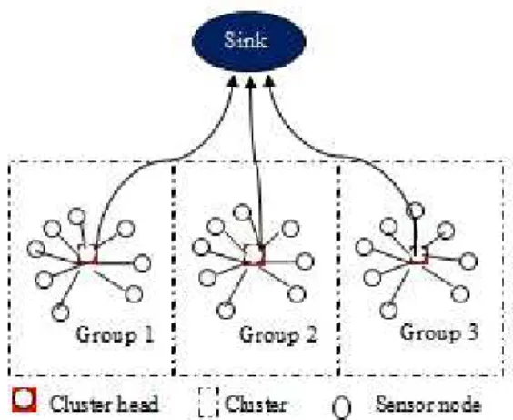
4.1 Cluster based sensor network . . . 58

4.2 Diagram of Feed Forward Neural Network . . . 59

4.3 Density Curves of CO, Temperature, Photoelectric and Ionization respectively. . . 63

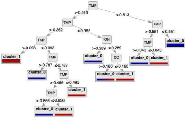
4.4 Diagram of Decision Tree . . . 64

5.1 Radio Energy Dissipation Model . . . 72

5.2 Covered Grid points in a 10×8 Sensing field . . . 75

5.3 Illustration of Nodes to Sleep on Coverage Area . . . 76

5.4 Step Size division of Search Length . . . 79

5.5 The operational sequence of the proposed clustering protocols . . 83

5.6 Network Lifetime Comparison of DLSACH with LEACH, SEECH, TCAC . . . 88

6.1 One round of the clustering process . . . 94

6.2 Sensor nodes Topology and Random distribution . . . 95

6.3 Binary representation of individuals in the population . . . 97

6.5 Average residual energy of nodes alive versus rounds (refer to ExpR0M100) . . . 104

6.6 Round number versus numbers of heterogeneous sensors . . . 105 6.7 Performance Comparison of different WSNs Heterogeneity Level

4.1 Distribution table for the four sensor types . . . 63

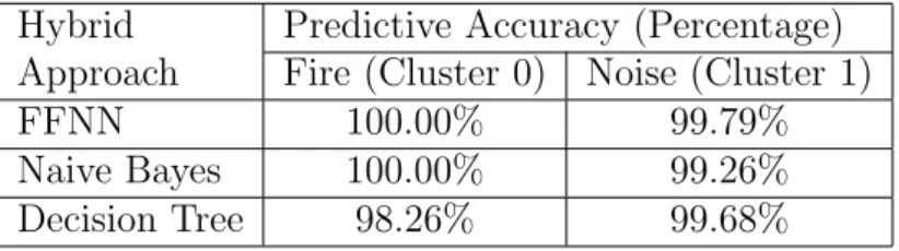
4.2 Empirical Results for all Classifiers . . . 65

5.1 Communication Parameters with Specified Values . . . 85

5.2 Parameter values for each experiment . . . 85

5.3 Comparison of LEACH, TCAC, SEECH andDLSACHfor FND,LND and IPL . . . 87

5.4 Performance Measures for Experiment III,IV and V . . . 87

6.1 Parameter settings for Homogeneous WSNs Scenarios . . . 99

6.2 Parameter settings for Heterogeneous WSNs Scenarios . . . 100

6.3 Performance comparison of LEACH, TCAC and SEECH with HACH101 6.4 AEFND of proposed HACH protocol . . . 103 6.5 Performance Measures for different heterogeneous WSN Scenarios 105

Acronyms

DLSACH Dynamic Local Search Algorithm for Clustering Hierarchy

HACH Heuristics Algorithm for Clustering Hierarchy

HEECHS Heuristic Enhance Evolutionary Algorithm for Cluster Head Selection

SSIN Stochastic Selection of Inactive Node

CHs Cluster-heads

CI Computaional Intelligence

DE Differential Evolution

DT Decision Tree

FFNN Feed-Forward Neural Network

GA Genetic Algorithms

GD Gradient Descent

HEED Hybrid Energy Efficient Distributive

ILS Iterated Local Search

LDS Linear Distance-based Scheduling

LEACH-C LEACH-Centralised

MA Memetic Algorithm

ML Maximum Likelihood

NBC Naive Bayes Classifier

NFDRS National Fire Danger Rating System

NN Neural Network

PSO Particle Swarm Optimisation

RS Randomized Scheduling

SA Simulated Annealing

SEECH Scalable Energy Efficient Clustering Hierarchy

TCAC Topology-Controlled Adaptive Clustering

TS Tabu Search

WSNs Wireless Sensor Networks

Symbols

Accef f Accumulated coverage effect

AvgECH Average energy of CHs

AvgEN CH Average energy of non-CHs

Cef f Coverage effect

d0 Threshold distance

EAggreg Energy consumed in aggregating measured data

ECH Energy consumed by Cluster heads

EM em Energy consumed by Member nodes

ERes Residual Energy

ERx Energy consumed by the transceiver to receive a data message

ET otal Total energy consumed by a wireless node

ET x Energy consumed by the transceiver to send a data message

k Packets

kCP Control packets

L Number of Cluster heads

mp mutation probability

M axef f Maximum coverage effect

R Risk penalty

Rs Sensing range

Introduction

1.1

Motivation

Recent progress in Micro-electromechanical Systems (MEMS) has enabled the development of self-configurable and spatially distributed autonomous sensors Naeimi et al. [2012]. These sensor nodes can be networked and deployed ran-domly in remote and inaccessible areas, hence producing useful wireless sensor networks (WSNs). In large areas, WSNs are used for gathering data from the sensor field and transmitting data to a distant sink. The potential applications of WSNs are environmental monitoring, target field imaging, weather monitoring, security, battlefield surveillance, event detection etc. The event detection is a newly discovered WSN functionality that offers extended capability of reporting data that contain time and location of events, which is contrast to periodic moni-toring that transfers data without any abnormal change of condition. The design of in-network event detection methods for wireless sensor networks is not an easy task, as there is a need to cope with various challenges and issues such as the unreliability, heterogeneity, adaptability and most especially resource constraints such as battery energy.

Energy efficiency and network lifetime are major issues that require consider-ation in the design of protocols for WSNs. The field of WSNs embrace innovative techniques that can eliminate energy inefficiencies that would shorten the network lifetime. Energy constraint is a major problem in WSNs most especially when

larger number of sensor nodes are deployed. The limited energy poses many chal-lenges to the design and management of WSNs and necessitates energy-awareness at all layers of the networking protocol stack. For example, at the network layer, it is highly desirable to find methods for energy-efficient route discovery and relay-ing of data from the sensor nodes to the base station (BS) so that the lifetime of the network is maximizedAbbasi and Younis[2007]. Most existing routing proto-cols designed to tackle the above challenges are broadly classified into two classes, namely flat and hierarchical. Flat protocols include the old-fashion Direct Trans-mission (DT) and Minimum TransTrans-mission Energy (MTE), which cannot promise a balanced distribution of the energy among sensors in a WSN. The drawback with DT is that sensor nodes communicate directly with the sink and this causes far away sensors to die first. In the MTE, far away sensors use a relay sensor for data transmission to the BS and this causes the relay sensor to die first.

Therefore, designing energy-efficient clustering protocols becomes a major fac-tor for lifetime extension of sensors. Generally, clustering protocols can outper-form flat protocols in balancing energy consumption and network lifetime pro-longation by adopting data aggregation mechanisms Abbasi and Younis [2007]; Heinzelman et al.[2002]. Theoretically, there are three types of nodes, namely the cluster-head (CH), member node (MN) and sink node (SN). The member node is responsible for sensing the raw data and employs TDMA scheduling to send the raw data to the CH. The main role of the CH is to aggregate data received from member nodes (MN) and thereby forwards the aggregated data to the sink through single-hop or multi-hop. CH selection can either be done by the sensors themselves, by the BS or can be pre-determined by the wireless network designer. From a theoretical and practical point of view, WSNs can be classified into the Homogeneous (WSNs with the same sensor node configuration e.g. Energy) and the Heterogeneous (WSNs with dissimilar sensor node configuration).

Reliability is another key issue that needs to be considered for some critical or event detection applications such as indoor fire detection, forest fire and pipeline monitoring etc. Fast and accurate fire detection helps to minimise fire losses that often results into loss of lives and damage to properties. Therefore, researchers have been investigating new techniques that will help in fast and accurate fire detection. For a system to decide accurately an abnormal condition such as fire,

there maybe a requirement to combine several attributes based on large number of sensor types (temperature, carbon monoxide (CO), smoke) which are spatially distributed over a wide area Memon and Muntean [2012]. Data obtained from a composite event are multidimensional in nature. One of the key measures of enhancing accurate fire detection decisions is to perform data aggregation at in-termediate nodes or at the cluster head. Data aggregation usually involves the fusion of data from multiple sensors at intermediate nodes and transmission of the aggregated data to the base station (sink). Data aggregation helps to remove redundant and highly correlated data generated from neighbouring sensors at the intermediate node before transmission to the base station Memon and Muntean [2012]. Data aggregation techniques are also very effective in reducing communi-cation overhead by collecting the most critical data from the sensors and making it available to the sink in an energy efficient manner with minimum data latency. Data latency is a crucial requirement in most event detection application such as fire detection applications.

1.2

Research Objective

The main objective of this thesis is to analyse, investigate applicability and timise computational intelligence methods for energy-efficient and intelligent op-erations of wireless sensor networks (WSNs). Therefore, in order to achieve the objectives, the research sub-objectives of this thesis are as follows:

1. Design a new protocol that is based on metaheuristic algorithms that can equally and efficiently distribute the energy consumptions evenly among sensor nodes and still achieve an extended network lifetime compared with the state-of-the-art designs often offered as solutions for a clustered archi-tecture in the literature.

2. Provide a comparative assessment of other state-of-the-art protocols with the new design protocol for lifetime extension purpose using a simulated environment.

can efficiently extract patterns and detect trends that are hidden in com-plex fire data sets. This objective aims at improving the detection accu-racy of fire detection systems compared with the current state-of-the-art approaches that has been used for the similar problem.

4. Provide a comparative study of state-of-the-art event detection techniques in terms of their detection rate and accuracy.

1.3

Thesis Contributions

The contributions of this thesis are:

1. The design and implementation of an energy-efficient transmission protocol for extending lifetime of wireless sensor networks.

2. The development of a sleep scheduling mechanism that is based on the Boltzmann selection process in genetic algorithms for conserving the energy of sensor nodes. The network coverage is analysed and put into considera-tions in the selection of inactive nodes.

3. The design of new WSN clustering protocol that employs metaheuristic approaches to distribute cluster head and energy loads evenly among sensor for the purpose of prolonging WSNs lifetime.

4. Perform data aggregation on three multi-dimensional datasets obtained from a real time fire scenario.

5. The proposal of new hybrid machine learning approaches for accurate event detection using k-means and other classification models.

1.4

Journal and Conference Publications

1. Muyiwa O. Oladimeji, Mikdam Turkey, Mohammed Ghavami and

San-dra Dudley, ”A New Approach for Event Detection using k-means Cluster-ing and Neural Networks”, IEEE International Joint Conference on Neural Networks, IJCNN 2015, Killarney, Ireland, July 12-17, 2015, Pages 1-5. DOI: 10.1109/IJCNN.2015.7280752

2. Muyiwa O. Oladimeji, Mikdam Turkey and Sandra Dudley, ”A Heuristic

Crossover Enhanced Evolutionary Algorithm for Clustering Wireless Sensor Network ”, EvoApplications 2016, Porto, Portugal, March 30 –April 1, 2016, Proceedings, Part I, Pages 1-16, 2016a. DOI: 10.1007/978-3-319-31204-017

3. Muyiwa O. Oladimeji, Mikdam Turkey and Sandra Dudley, ”Iterated

Local Search Algorithm for Clustering Wireless Sensor Networks”, IEEE Congress on Evolutionary Computation, CEC 2016, Vancouver, BC, Canada, July 24-29, 2016, Pages 3246-3253, 2016b. DOI: 10.1109/CEC.2016.7744200

4. Muyiwa O. Oladimeji, M. Turkey and S. Dudley, “HACH: Heuristic

Algorithm for Clustering Hierarchy Protocol in Wireless Sensor Networks”, Applied Soft Computing Journal, Volume 55, Pages 452–461, 2017. DOI: 10.1016/j.asoc.2017.02.016

1.5

Thesis Organization

The rest of this thesis is organised as follows:

Chapter 2 reviews wireless sensor networks (WSNs) and these applications, requirements, challenges and energy consumption. The chapter reviews the re-cent sleep scheduling and clustering mechanisms for the design of energy-efficient WSNs. As a subset of computational intelligence, a review on the different meta-heuristic optimisation algorithms as presented in this chapter. Finally, the chap-ter reviews optimisation of energy-efficient cluschap-ter-based WSNs using metaheuris-tic approaches.

Chapter3introduces the use of WSNs for monitoring or event detecting appli-cations such as fire detection system. It discusses the problem of traditional fire detection techniques and the introduction of WSNs into fire detection systems. It discusses new trend of incorporating artificial intelligence-based techniques into WSNs-based fire detection system for improved performance. Finally the chapter reviews various AI-based techniques under the machine learning approaches for fire detection applications.

Chapter 4 proposes a new hybrid approach to event detection that combines data aggregation,k-means clustering and supervised machine learning approaches such as feed forward neural network (FFNN), Na¨ıve Bayes (NB), Decision Tree (DT).

Chapter5presents a new local-based metaheuristic approach for energy opti-misation in WSNs called Dynamic Local Search Algorithm for Clustering Hierar-chy (DLSACH). Under the DLSACH algorithm, the Stochastic Selection of Inactive Nodes (SSIN) and Iterated Local Search Algorithm for Cluster Head Selection (ILSACHS) protocols are proposed and they work cooperatively to minimise the energy consumption and extend the WSNs lifetime. The algorithms are evaluated via simulation experiments and compared with some existing algorithms.

Chapter 6propose the Heuristics Algorithm for Clustering Hierarchy (HACH). It introduce the SSIN mechanism proposed in the previous chapter for sleep scheduling operation and a novel heuristic crossover operator to combine two different solutions to achieve an improved solution that enhances the distribution of cluster head nodes and coordinates energy consumption in WSNs. It presents the performance in terms of lifetime extension under various WSNs conditions.

Chapter7closes the thesis, reviewing the work undertaken and draws conclu-sions about key parts of the work presented. Finally, future work is discussed.

Energy Efficiency Mechanisms

for WSNs

This chapter presents a background on wireless sensor networks and the state-of-the-art energy saving mechanisms in WSNs. It covers aspects of WSNs such as components, applications, prominent challenges and energy consumption models. A review on the design energy-efficient WSNs using all the different classifications of sleeping and clustering techniques is discussed. Also, a review on the different meta-heuristic optimisation algorithm, which are the subset of computational intelligence. Lastly, this chapter presents a review on the design of cluster-based energy efficient WSNs using meta-heuristic search strategies.

2.1

Introduction

Wireless Sensor Networks (WSNs) have grown to be a powerful technological platform with vast and profound applications. They have transformed into an important technology with many simple and complex applications such as envi-ronment monitoring, surveillance systems and military operations. A WSN usu-ally consists of tens to thousands of sensor nodes that communicate via wireless medium for the purpose of sharing and processing data Yu et al. [2006]. Sensor nodes are usually deployed randomly in a sensor field. They wirelessly commu-nicate with each other to coordinate themselves in order to produce reliable and

precise information about the physical environment under their coverage.

Each of the sensor nodes act independently to collect and route data to other sensors or the base station (BS). The base station is usually an intelligent device with unlimited energy resources that is capable of connecting the sensor network to an external communication infrastructure or internet for easy usage of the re-ported data for decision making. It is also the point where aggregation, clustering and routing tasks are implemented for a dense WSN (high node density). Usu-ally, sensor nodes can be deployed stationary or mobile over large areas. Though the sensor nodes can work autonomously, they work cooperatively to sense the physical conditions of an environment. Sensor nodes can sense the environment, communicate with neighbouring nodes, and in many cases perform basic com-putations on the data being collected Akkaya and Younis [2005]; Zungeru et al. [2012]. These attributes qualify WSNs to be an excellent choice for many appli-cations Yu et al. [2006].

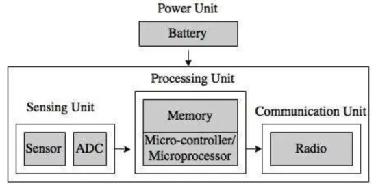
Sensors consist of four basic unit components: a sensing unit, a processing unit, a communication unit, and a power unit as shown in Figure 2.1. The sensing unit usually consists of sensor(s) and an analogue to digital converter bits (ADC). In sensing applications (such as weather monitoring, tactical surveillance, event detection etc), the sensor nodes sense or measure the physical condition of a monitored area. The ADC digitises a continuous analogue signal sensed by the sensors before sending it to the processing unit. This unit is made up of the memory-enabled micro-controller/microprocessor which provides the sensor nodes with intelligent control capabilities. The communication unit consists of a short-range radio capable of transmitting and receiving signal over a channel. The power unit is made up of a battery for supplying power that drive rest of the built-on system components Al-Karaki and Kamal [2004]. However, one of the issues that sensors have is the limited energy supply of the battery and so there is need to employ energy conservation strategy in order to prolong the lifespan of sensors.

Routing is a major process to be considered in order to minimise the energy consumption in WSNs. Due to the limited transmission range of each node, it may be necessary for sensors to use other nodes to forward packets to the BS. Routes discovery and maintenance in WSNs is non-trivial due to the energy restrictions

Figure 2.1: The components of Sensor node

and transmission range restrictions. To minimise energy consumption, routing protocols proposed in the literature for WSNs employ some well-known routing strategies such as clustering.

Clustering protocols in WSNs aim at grouping the sensors into clusters and selecting a cluster head (CH) for each cluster. In order to realise an energy efficient WSN, the CH can aggregate the data sent from the cluster members and send them directly to the BS. A clustering protocol is mainly a two layer protocol. The first layer deals with deciding the optimal CH set and the second layer protocol is responsible for transmitting the data to the BS. The clustering protocol in WSNs should not only facilitate data transmission, but also consider the sensor nodes’ constraints. It should also meet the WSNs requirements including the energy efficiency, the data delivery reliability, and the scalability requirements (see section 2.1.2). Apart from clustering, the sleep scheduling mechanism is another energy saving technique that preserves the lifespan of sensors by causing sensor to sleep when not needed and awake or active intermittently. More details on sleep scheduling is covered in section 2.2.

2.1.1

Applications of WSNs

WSNs are used for different applications ranging from military to civil application such as medical, industry and home Puccinelli and Haenggi [2005]. The various

applications can be categorised under the following sub-headings.

Environment Monitoring Systems

Environment monitoring systems are a crucial application that control and mon-itor environment conditions such as light, pressure, humidity and temperature Othman and Shazali [2012]. Applications have grown rapidly for monitoring pur-poses such as indoor, greenhouse, agriculture, climate, habitat and forest moni-toring. In Chang et al.[2012]; Lazarescu [2013]; Nie et al. [2014], several studies have been focused on this application aspect. The major WSN requirements of environment monitoring applications arescalability, coverage and energy

ef-ficiency. Apart from the previously mentioned requirements, there is need for

data reliability in the case of indoor monitoring applications such as fire detec-tion and alarm systems because it involves property and the protecdetec-tion of life. Monitored areas can span up to several square meters, so the number of nodes deployed over an area can vary from hundreds to thousands. Hence, scalability is a very important pre-requisite in the development of any protocols that can support very large quantities of nodes and guarantee full coverage of the moni-tored areaRault et al.[2014]. The protocols proposed in this thesis are applicable for environment monitoring because they put into perspective the three essential design requirements; which are lifetime extension, coverage and reliability.

Human Body Monitoring

Research interest in the aspect of wireless health care systems has grown rapidly and contributed advantageously to increasing numbers of elderly people, ability to place patients under continuous health monitoring and the rising cost of med-ical services. The emergence of novel wireless human body monitoring system such as wireless body sensor networks (WBSNs) have unlocked the potential to a broad variety of assisted living applications such as biochemical/biophysical con-trol, emotional recognition for social networking, activity monitoring for health care, e-fitness, emergency detection, security, and highly interactive gamesAiello et al. [2011]. Lots of efforts has been geared toward WBSNs for human body monitoring by researchers Baskaran [2012]; Gulcharan et al. [2014]; Kateretse

et al.[2013]. Human body monitoring is conducted using WSNs which is usually attached to the body surface and planted inside the human body tissue. Mod-ern technologies have produced micro and intelligent medical sensors that can be worn or implanted into the body. The sensors extract data from different parts of the body systems and send it to a central device that performs aggregation and analysis. These applications require high reliability due to the involvement of human’s life Souil and Bouabdallah [2011]. Another very important require-ment that ensures lengthen period of system operation is the network’s energy efficiency Baskaran[2012]; Souil and Bouabdallah [2011].

Intelligent Buildings

Intelligent and automated buildings is a WSN application that address increasing energy cost and aiding the green movement. Smart sensor nodes that can improve safety and security, minimise energy consumption and operational costs have been deployed for building automation applications. Using WSNs, Several literatures in Dounis [2010]; Fortino et al. [2012]; Suryadevara et al. [2015] have proposed several intelligent building management systems. In WSNs, different sensor types that measure parameters such as pressure, temperature, smoke and light are em-ployed for intelligent building management systems. At different level and home appliances, this system may include servers, gateways, actuators, communication and application software Jaafar and Watfa [2013]. Intelligent building manage-ment systems require multi-hop communication approach for covering the whole building. Another vital system requirement for this purpose is the WSNs energy efficiencyJaafar and Watfa[2013]. Some hierarchical or data-centric protocol can be used to satisfy these requirement Fortino et al. [2012].

2.1.2

Requirements and Challenges of WSNs Design

WSNs consist of a large number of sensor nodes that are made up of miniature devices constrained in their stored energy capabilities. Therefore in order to increase their usefulness, energy efficiency is a pivotal system requirement in WSNs. WSNs should put into consideration the sensor nodes’ short transmission range in the sending data to the sink. Data reliability is another core requirement

that must be considered in WSNs design. Clustering facilitates local interaction among sensor nodes in a coordinated manner which enables the WSNs to achieve the utmost goals such as scalability and efficient usage of limited energy resource Tubaishat and Madria [2003]. Scalability simply means the system ability to work efficiently with improve performance as the network size increasesLee et al. [1998]. Thousands of sensors are deployed in a large area of interest to compensate for the limited transmission range of each sensor. The most preferable routing scheme in WSNs is the one that can work efficiently with this large number of sensor nodes and must be capable of adapting to an increasing network size. Therefore, scalability is a another major requirement in the WSNs system design. To measure the performance of any clustering protocol in terms of scalability, the number of un-clustered is recorded as a performance metric. An increasing quantity of un-clustered nodes indicates a degrading performance in terms of the protocol scalability. WSNs researchers faces some challenges due to the unreliable nature of wireless communication and the limited resources of sensor nodes. The main challenges of the WSNs are listed as follows:

Limited Energy

Constrained energy supply poses a big challenge in the design of WSNs because sensors are powered on battery which has limited energy capacity. When the battery-energy of a sensor is depleted below a certain threshold, it becomes faulty and unable to work properly which can negatively affect the overall network performance. Due to the small size of sensors, batteries are usually designed in small sizes. Therefore, the overall operation of sensors is limited by the available battery energy. On the contrary, sensors need to continuously sense or collect, transmit and receive data for a long period of time. To ensure that sensors operate for long period of time, the battery energy must be managed efficiently. Consequently, the routing protocols adopted by sensor networks should achieves the energy efficiency requirement so as to minimise the energy consumption and hence extend the network’s lifetime. Although, WSN applications faces different issues but the common challenge is the limited energy. Energy consumption is considered the main challenge for WSN operation. The sensor nodes are equipped

with limited batteries. They are deployed in hostile or unsafe areas; making recharging or replacing the battery unfeasible, hence the need to conserve battery energy Raghunathan et al. [2002].

Every node operation consumes energy. Energy is consumed in sensing, pro-cessing and communicating. Sources of energy consumption include:

ˆ Idle: It reflects the time during which the node keeps listening to the

channel waiting to receive data. The idle process consumes energy which can be considered as passive. The node could be designed to sleep during passive time and wake-up to receive data. Designing node’s duty cycle to sleep and wake-up at the right time is still a challenge.

ˆ Data Aggregation: Sending data messages from all sensors to the base

station directly causes overheads due traffic congestion. Aggregating data can reduce communication traffic. This is done by combining data messages into one. Data aggregation requires the node to have sufficient memory, processor capabilities and energy for processing.

ˆ Communication: Most of the node’s energy is consumed during

commu-nicationHalkes et al.[2005]. The consumed energy during communication is affected exponentially by the distance between the communicating nodes; the longer the communication distance between sensors the more energy is consumed. In order to save energy, communication distance should be minimised. Moreover, designing a suitable pattern for the antenna help reducing energy waste. It was reported that the energy consumed for an antenna pattern to reach all hosts is proportional to the area it covered Sravan et al. [2007].

Short Transmission Range

Each sensor needs to transmit their data to the sink even though their trans-mission range is limited. The sink is normally fixed and located far away from the sensors. In addition, the link quality between the sensors nodes and the sink need to be enhance in order to facilitate network throughout and data reliability.

Clustering techniques that uses multi-hop communication approach is the best strategy that can satisfies this requirement.

Coverage Problem

Coverage can be defined as the extent or degree to which each grid point of network area is covered by a sensor node. The coverage problem is whether each or every point in the target or area of interest falls within the sensing range of the deployed sensors Sangwan and Singh [2015].

Scalability Issue

WSNs can consist of a large number of sensor nodes with high node density. Designers find it a great challenge designing a scalable protocol that can work efficiently at such a large network size.

Cluster and Route Optimisation Issues

In WSNs, there is a need to apply the best clusters that can route traffic in an energy efficient manner such that the overall energy consumption is minimised and the sensor lifetime is extended. The clusters formation and cluster head selection among the sensors is regarded as an optimisation problem that can be tackled using meta-heuristic algorithms (Refers to Section 2.4).

2.1.3

Energy Consumption in WSNs

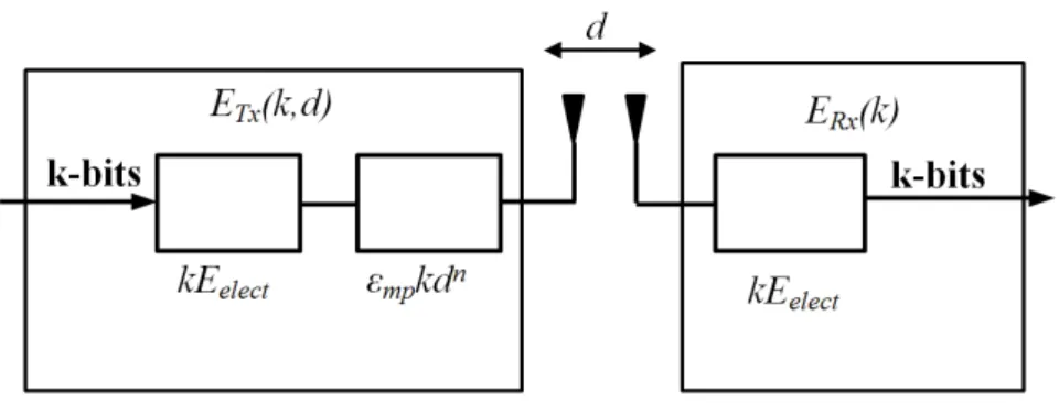
As mentioned earlier, a wireless sensor node consists of: sensing unit, processing unit, transceiver and power supply. The power supply provides energy to all other sensor components. The sensed measurements are converted to a digital signal by means of the analogue-to-digital converter (ADC) of the sensing unit. The processing unit aggregates the digitised data into one single message to be sent by the transceiver. The total energy consumed by a wireless sensor is the amount of energy required to perform sensing, aggregation and transceiver operations. Typical operations of the transceiver are: sleep, idle, transmit and receive. The

total energy consumed is computed as:

ET otal =ESU +EAggreg +ESleep+EIdle+ET x+ERx (2.1)

Where:

ˆ ET otal is the total energy consumed by a wireless node,

ˆ ESU is the energy consumed by the sensing unit,

ˆ EAggreg is the energy consumed in aggregating measured data,

ˆ ET rans is the total energy consumed by the transceiver,

ˆ ESleep is the energy consumed by the transceiver during sleep operation,

ˆ EIdle is the energy consumed by the transceiver while in the idle state,

ˆ ET x is the energy consumed by the transceiver to send a data message,

ˆ ERx is the energy consumed by the transceiver to receive a data message.

Sensors spends most of its energy to transmit and receive packets whereas the energy consumed during the idle, sleep states and sensing unit is negligible (ESleep,EIdle andESU is approximately zero). Equation2.1can be approximated

to:

ET otal =EAggreg +ET x+ERx (2.2)

2.2

Sleep Scheduling Mechanisms Overview

In WSN environments, sensor node sleep scheduling can be used as an energy conservation method for network lifetime extension. This section present few notable energy-efficient scheduling mechanisms in sensor networks.

Randomized Scheduling Scheme

In the randomized scheduling (RS) scheme, sleeping sensors are selected randomly in a given cluster with a probability ofp=βs<1 (whereβsis the average fraction

of sensors allowed to sleep). This scheme is very simple to implement. Each sensor only needs to examine the data obtained from a biased random generator to decide whether to turn into sleep mode or not. All sensors in the cluster have

same sleep probability. The major drawback with this scheme is that more energy is consumed if the sensors at cluster boundaries are kept active and this can also leads to variation of energy consumptions by all sensors. This sleep scheduling scheme is only suitable for single-hop cluster-based sensor networks with variable transmission power Deng et al. [2005a].

Linear Distance-based Scheduling

A sleep-scheduling algorithm called Linear Distance-based Scheduling (LDS) scheme for cluster-based high density sensor networks was proposed in Ramesh et al. [2012]. The goal is to reduce energy consumption without affecting the coverage capabilities of the sensors. This goal is satisfied by causing sensors that are far away from the cluster head to become inactive with higher probabilities. Also, experimental result shows that the LDS scheme is better than the RS in that the sensing coverage of sensors at the border area are lower than the central area of the cluster Deng et al. [2005b]. The idea behind this scheme is that more sensor energy can be saved by allowing far away sensors to sleep for longer periods com-pared with sensors that are closer to the cluster head. According to Deng et al. [2005a], the probability p a sensor goes into sleep mode is given as:

p(x) = 2Rβs 4 2x R2 = 3βsx 2R , 0≤x≤R (2.3)

Where R is the communication range between CH and all sensors at maximum transmission power, βs is the fraction of sensors allowed to sleep (at < 2/3).

The sleep probability p of sensors is a function that is dependent on x, which is the distance of a sensor from its respective cluster head and x is a value within sensor’s communication rangeR. The LDS scheme works only with static clusters (CHs remain the same throughout an operation once they are selected).The LDS scheme lowers the variation of energy consumptions compared with the RS scheme Deng et al. [2005a].

Balanced-energy Sleep Scheduling

This scheme employs the base station to extend the LDS scheme by evenly dis-tributing the sensing and communication tasks among the non-head sensors so that their energy consumption is similar regardless of their distance to the cluster-head Le et al. [2008]. This scheme employs a sleep probability function p(x) so that the total energy consumption of a sensor does not depend on x, the distance between sensor and its CH. The main goal of this scheme is to use a sleep proba-bility that provides balanced energy consumption for a larger portion of sensors in a cluster thereby reducing the overall energy consumption. More details about this scheme is provided in Deng et al.[2005a]

Other Sleep Scheduling Mechanisms

In Danratchadakorn and Pornavalai [2015], a coverage maximisation with sleep scheduling protocol (CMSS) that ensures network areas are fully covered by se-lected active sensors was presented. Each sensor exchanges information with its neighbouring sensors and sets a waiting time. During sensor waiting times, a sen-sor can receive a sleep message from neighbouring nodes. When a sensen-sor receives these messages, it updates its own neighbour and cell value table. If the minimum value of the cell value table of a sensor equals to one, it silently becomes an active node. Otherwise, it will wait for the waiting time to expire before it turns into an inactive node. An energy preserving sleep scheduling (EPSS) strategy allows each sensor to make decision regarding going into sleep mode based on their distance from the cluster head and network density. This guarantees balanced energy con-sumption in the cluster by taking into account the density of node deployment and the network load while determining the sleep probability Singh and Lobiyal [2013]. In Bulut and Korpeoglu[2011], a probabilistic and analytical method was employed to approximate the overlapping sensing coverage between a node and its neighbours. It also estimates when a node can be put into sleep without jeop-ardizing expected coverage. The method is employed by the proposed scheduling and routing scheme to diminish control message overhead while considering the next mode (full-active, semi-active, inactive/sleeping) of sensor nodes.

2.3

Clustering Mechanisms Overview

Clustering is a key mechanism in large multi-hop wireless sensor networks for obtaining scalability, reducing energy consumption and increase in the network lifetime to achieve improved network performance. In Abbasi and Younis[2007]; Tyagi and Kumar [2013]; Younis et al. [2006], Clustering techniques have been studied extensively to improve the performance of WSNs. In this section, several traditional clustering protocols were presented, which includes the Low Energy Adaptive Clustering Hierarchy (LEACH), Topology Controlled Adaptive Cluster-ing (TCAC), Scalable Energy Efficient ClusterCluster-ing Hierarchy (SEECH) and other clustering approaches.

2.3.1

Low Energy Adaptive Clustering Hierarchy (LEACH)

LEACH is one of the most common cluster-based routing protocols in WSNs that has been proven to be an effective approach to prolong the network’s lifetime Heinzelman et al. [2002, 2000]; Tyagi and Kumar [2013]. The LEACH protocol was published in a seminal paper byHeinzelman et al. [2002], and has been cited in most research papers of similar research area. This is a completely distributed approach that does not require a global information of the network. The basic idea of LEACH has been an inspiration for many subsequent clustering protocols. The main objective of LEACH is to equalise the energy load distribution among the CHs. LEACH lifetime operations is made up of several rounds and each round consists of two phases, namely the set-up phase and the steady-state phase. In the set-up phase, the clusters are organised, while in the steady-state phase, data is delivered to the BS. The steady-phase span through longer period compared with the set-up phase in order to reduce overhead. For each, the node decide whether to be the CH or not at the set-up phase. This CH decision is based on the percentage allocation of CHs or the number of times the sensor has been a CH. Cluster-heads can be chosen stochastically (randomly based). At the set-up phase of each round, a stochastic threshold valueT(n) is computed at each round

as defined below: T(n) =    P 1−P×(rmod_P1), if ∀n ∈G 0, Otherwise (2.4)

Where n is a random number between 0 and 1, P is the desired CHs percentage, r is the current round, and G is the set of nodes that have not been elected as CHs in the last _P1 rounds. During set-up phase, each sensor nodes will select a random number n between 0 and 1. This random number n is compared with T(n) and if it satisfies the condition n < T(n), the node becomes a CH. This LEACH protocol ensures that every node becomes a CH exactly once within 1

P

rounds.

When a cluster head role is assigned to a node and this node announces its new role to other nodes via an advertisement message. All the nodes decide which CH to join based on the received signal strength of the advertisement message. Each node responds to their respective CH via a membership message. Using equation 2.4, the CH role is decided in order to distribute the energy load among sensors. During the steady-state phase, the sensors transmit data packets continuously to the CHs. Each CH aggregate all the data received from all its member nodes and this aggregated data is sent to the BS directly. To avoid inter-cluster and intra-cluster collisions, LEACH employs Time Division Multiple Access (TDMA) technique. After a time duration or round length, the WSNs begins another round starting with the set-up phase where new CHs are elected.

The idea behind LEACH is that any node that has been appointed as CH in a round can not be elected as CH again. This LEACH scheme enables each node to share equally the extra energy load imposed by acting as the CH. However, the drawback is that LEACH can not guarantee equal load-balancing in the sense that sensors are elected as CHs based on probabilities without considering their energy value while choosing T(n). In addition, selecting the CHs randomly does not gives an even distribution of CHs over the WSNsArboleda and Nasser[2006]. Another drawback is that LEACH assumes a single-hop communication with the BS, which is unrealistic in many practical scenarios due to the restricted communication range of sensors Saleem et al. [2011]; Zungeru et al. [2012]. An

attempt to increase the transmission range can also cause sensors to consume more energy for transmission.

2.3.2

Topology Controlled Adaptive Clustering (TCAC)

The TCAC protocol consists of three phases namely the periodical update, clus-ter heads election and clusclus-ter formation Dahnil et al. [2012]. At every network operation round, each sensor dynamically changes its transmission power level Ptx. At the start of periodic update, each sensor successively broadcasts an

up-date message containing its ID, at each power level. Other sensors will send an acknowledgement (Ack) after receiving the packets. Sensor’s degree is computed based on the number of received Acks. The broadcasting sensors must perform many transmissions to obtain a power level that is equivalent to the degree thresh-old (Qmin). To preserve the network connectivity at a given number of sensors

n, the degree threshold Qmin is defined as:

Qmin = 5.1774 logn (2.5)

According toXue and Kumar [2004], the relevance of Equation 2.5 is that as each sensor is connected to more than 5.1774 lognnearest neighbour, the network is asymptomatically connected with a probability approaching one as n increases. For instance, if a sensor’s degree is less than the degree thresholdQmin, then the

sensor must increase its power level. Alternatively, if the sensor’s degree is greater than the threshold, then the sensor must reduce its power level until Qmin is

achieved. This attainable power level by the broadcasting sensors is set as the base power level. This information will be stored in the sensor’s cache for clustering operations. The cluster heads are elected in the second phase of TCAC protocol in three sequential steps. In Step 1, a sensor computes its probability (P(CCHi))

to become CH candidate based on its remaining energy Ei with respect to the

average energy Eavg of all sensors in the WSNs. LEACH protocol defines the

optimal number of cluster headskoptthat can achieve minimum energy dissipation

per round. A parameter kinitial that can obtain non-overlapped CHs is defined

The probability of a sensor to be elected as a CH candidate is computed as follows

P(CCHi) =

Ei

Eavg

(2.6)

And Eavg is calculated as follows

Eavg =

Etotal

kinitial

(2.7)

Each sensor generates a random number in the range of [0,1] and if the number is less than the calculated probabilityP(CCHi), it elects itself as a candidate CH.

Other sensors that are not elected will wait to receive membership message from the newly elected CH. At the end of each round, all member sensors send their residual energy to their respective CH, which aggregate the values and update the rest of CHs in the network. Based on the received information, the CHs compute Eavg value. The information is sent to all sensors in order to compute

the P(CCHi) for the next round of network operation. There is a higher chance

that sensors elected as CH in previous round may not be elected in the next round due to higher energy spent for communication with the base station. In Step 2, the candidate CHs obtained in Step 1 is compared against each other and the condition below must be satisfies for CH election.

ˆ The CH candidate with a higher energy is re-elected as a CH and the other candidates becomes a member nodes.

ˆ If the energy of two candidate CHs is the same, then the candidate CH with higher degree is re-elected as the CH.

In Step 3, CHs set power level Ptx through Ack counts received from

trans-mission in order to update the sensor’s degree. If the sensor degree correspond to the Qmin, the CH transmit a cluster head message CHMSG its new role. In

the cluster formation phase, the non-CHs respond back to CH with a request messageREQMSG containing its ID. Sensors that do not receiveCHMSG across the network send request message to CHs after the time has expires. CH rank members based on the received signal strength of REQMSG and stored them in a priority list in the structure (ID, Rank). At the top of priority list is the

sensor with strongest signal strength. CH broadcast the priority list to all sensors requesting to join its cluster. The two important facts can be deduce from the priority list:

1. Sensors are aware about their closeness to the CH compare to other sensors requesting to join the cluster,

2. Sensor may join cluster to fulfil the threshold degree of CH rather than considering the closeness to CH. From the list, non-CH nodes compute the degree of each CH and a sensor joins cluster that has a lower degree than the Qmin.

In situation where the degree of all cluster heads are equal or greater than the Qmin, the sensors compare ranks given by all CHs and join the cluster that placed

it in the best rank. After joining the cluster, member sensors adjust their trans-mission power for efficient intra-communication with CHs.

2.3.3

Scalable Energy Efficient Clustering Hierarchy

(SEECH)

After sensor deployment in a network area, The SEECH protocol starts operation at the start phase before the first round. Each sensor computes its distance from the sink and the number of neighbouring sensors ni in a specific radius RN G

Tarhani et al. [2014]. This obtained data is shared with other sensors and each sensor computes its degree degi as follow

degi =

ni

max(n1, n2, ..., nN)

(2.8)

Where nN is the overall number of sensors in the network. In SEECH protocol,

sensors with larger degrees are more suitable choices for cluster head. The merit of this approach is that large number of member nodes is covered by small number of CHs using low power communication. The CH selection starts by electing some tentative CH using distributive method. In this method, each node i calculates

pci which describes the chances of being a tentative CH as follows: pci =    E_resi×degi pc−tot , if Eresi ≥Eav(1−λ) 0, else (2.9)

Where the Eresi denotes the residual or available energy of sensor i. λ is a

number in the range [0,1] and is usually set to 0.9 in order not to reduce the chances of low energy sensors. pc−tot is define as follows:

pc−tot = Eav× P Ndegi 2KCHC (2.10)

The pc−tot value assures that the number of tentative CHs will not be less

than the number of needed candidates (KCHC). In equation 2.10, Eav is the

average residual energy of the nodes in the current round which is calculated and broadcasted by cluster heads in previous round and during cluster formation. In each round, residual energy of nodes is in a small range; whereas, their degrees might be completely different e.g. degree of a node might be multiple times of another one. As a result, prioritizing the nodes by equation 2.9 is more heavily dependent on node degrees rather than residual energy. When pci is computed,

each sensor generates a random number in the range [0,1] and compares it with pci. If the random number is less than the pci, the sensor consider itself as the

tentative cluster head. All tentative CHs inform other tentative CHs and sensors by broadcasting a CH-CANDIDATE-MSG message using CDMA protocol. Each sensor receive the message and estimate its distance from the transmitting node. Prior to announcing its candidacy, each sensor counts the number of candi-dates and if it is equal to KCHC, it will not introduce itself as a candidate to

the network and gives up the competition in order to maintain constant num-ber of candidates. Each CH-CANDIDATE-MSG message which includes the ID, residual energy of sender and distances smaller than RNG from all previously introduced candidates in current round and corresponding IDs. The set of can-didates and cluster heads is denoted by RCHC and RCH and KCH is the number

of needed cluster heads. To eliminate each candidate, all candidates are scored once. The candidate with lowest score will be eliminated from the list. The same procedure will be repeated ignoring distance from eliminated candidate. The

pro-cess will continue till the number of remained candidates equals to the number of needed cluster heads. The SEECH protocol can execute algorithm in two ways. In the first method one candidate executes desired algorithm and announces fi-nal cluster heads. In the second method all candidates separately execute the algorithm and figure out their state themselves.

A sensor accepts the role of relay node only if it satisfies two conditions. Firstly, the sensors that are closer to the sink minimise transmission cost. Proto-cols must avoid selecting this sensor as cluster head. Secondly, since competence of electing a CH is proportional to node degree (which is number between 0 and 1), 1-degree is utilised and defined as the relay sensors. The procedure of selecting relay nodes is similar to selecting cluster heads. First of all, each node excluding cluster heads, calculates its chance of becoming a tentative relay node, pri, as

follows: pci =    E_resi×(1−degi) pr−tot , if Eresi ≥Eav(1−λ) 0, else (2.11) Where pr−tot = Eav× P N(1−degi) 2KR (2.12)

Thepr−tot value assures that the number of tentative relay sensors will not be

less than the sufficient number of tentative relay sensors (KR). In Equation2.11,

Eresi is included to protect low energy nodes. Whenpri is computed, each sensor

generates a random number and compares with pri. If the number is smaller

then the sensor becomes a tentative relay sensor. The relay sensor introduce themselves to the network by broadcasting a RLY-MSG message which consist of the node ID and residual energy. CHs also receive the message and decide the closest relays based on the signal strength. After the lowest energy nodes has been eliminated, the CHs chooses closest relay nodes among the tentatives and informed the elected relay about their choice by sending CH-NEXTHOP-MSG message.

Cluster formation process starts by CHs broadcasting a CHMSG message with the spreading code and ID. Each normal sensor chooses the closest CH

according to the signal strength. Afterwards the sensor informs the CH of its decision by transmitting a JOIN-MSG message which consists of node ID and cluster head ID, thereby forming clusters. CHs count their members based on the number of received JOIN-MSG messages and employ TDMA to collect cluster information. Therefore, each CH broadcast a SCHEDULE-MSG message with a radius equivalent to the distance of farthest sensor member. Using the messages CHs issue time-slots for each members to send its information. Also the average residual energy of the network is informed to the nodes by these messages. Now setup phase finishes and steady-state phase starts in accordance with determined topology.

2.3.4

Other Clustering Approaches

Another variant of LEACH protocol was proposed in Heinzelman et al. [2002], which is calledLEACH-centralised (LEACH-C). Unlike LEACH, LEACH-C employs the sink to perform the task of CH selection and formation. Each node sends their location and energy level to the sink. The sink employs a simulated annealing (SA) approach to determine the CH number and cluster configuration based on the received information. The energy and distance between CHs and non-CHs are considered for even load and cluster distribution. The sink optimises global knowledge of the network to produce an improved network that requires less energy. However, it assumes that the CHs can send aggregated data streams directly to the sink which is a similar drawback to LEACH. A hybrid energy

efficient distributive (HEED) protocol was proposed in Younis and Fahmy

[2004]. CH selection is achieved by iteratively considering the residual energy and the proximity to member nodes. In this protocol, the energy consumption for communicating between the CHs and non-CHs is reduced considerably and each CH communicates with the sink using multi-communication approach. How-ever, more CHs are generated than the expected number and this results in an unbalanced energy consumption. Also, HEED results into overhead since it does several iteration to select CHs.

In Smaragdakis et al.[2004], a stable election protocol (SEP) was devel-oped for the two level heterogeneous networks, which includes two types of nodes,

normal and advanced nodes. In SEP election probabilities are weighted by the ini-tial energy of a node relative to that of other nodes in the network. This prolongs the time interval of FND that must be crucial reliable communication. Further SEP is dynamic therefore it does not assume any prior distribution of the different levels of energy in sensor nodes. Finally SEP is scalable as it does not require any knowledge of the exact position of each node in the field. Disadvantage of SEP is that it performs poorly in terms of stability for multi-level heterogeneous WSNs. An energy-aware adaptive clustering protocol used in heterogeneous wireless sen-sor networks nameddistributed energy-efficient clustering (DEEC)scheme was proposed in Qing et al. [2006]. In DEEC, every sensor node independently elects itself as a cluster-head based on its initial energy and residual energy. To control the energy expenditure of nodes by means of adaptive approach, DEEC use the average energy of the network as the reference energy. Thus, DEEC does not require any global knowledge of energy at every election round. Unlike SEP and LEACH, DEEC can perform well in multi-level heterogeneous wireless sensor networks as shown in experimental results presented in Qing et al. [2006].

2.4

Metaheuristic Algorithms

Meta-heuristic approaches are widely employed as an efficient solution for many optimisation problems. They are defined as a heuristic process that intelligently combines diverse concepts in order to exploit and explore the search space, learn strategies that are tailored for finding solution close to the optimal solution El Emary and Ramakrishnan [2013]. The meta-heuristics algorithm is classi-fied into two types based on the search strategy namely the global and local heuristic search. Here, a brief overview of widely known global search meta-heuristics is presented: Genetic Algorithms (GA), Particle Swarm Optimisation (PSO), Differential Evolution and the Local search metaheuristics: Simulated annealing (SA), Iterated Local Search (ILS), Tabu search. Lastly, the Memetic algorithm (MA) , which is a hybrid approach of the global and local search strat-egy.

2.4.1

Global Search Strategy

The global search strategies are also refers to as the population-based meta-heuristics. Population-based approaches maintain and improve multiple candi-date solutions, often using population characteristics to guide the search. The global search provides the broad exploration mechanism. Algorithms under the population based metaheuristics include Genetic Algorithm, Particle Swarm Op-timisation and Differential Evolution.

Genetic Algorithms

Genetic algorithms have been in existence earlier than 1975, but it was intro-duced to the broad research community in a seminal paper by Holland [1975]. The genetic algorithm concept is a metaheuristic that imitate the process of nat-ural selection and the survival of fittest. In GA, solutions are represented as chromosomes. Using a fitness function, the quality of this chromosomes are eval-uated and eventually graded from the best to worst based on the obtained fitness value. To produce high quality solution for optimisation and search problems, the GA mimic three major natural selection operation of living organism such as selection, crossover, and mutation. To drive the GA process towards survival of the fittest, higher selection probability is assigned to chromosomes with better fitness. The selection probabilities are computed by ranking the fitness values of all chromosomes in a population relative to one another. The selection operator is applied to a population pool in order to select parent chromosome pair with the best fitness value. Afterwards, the crossover operator is applied to this pair, thereby producing a new offspring. Since the process is continuously driven to-wards the stronger (fitter) chromosomes, there is a likelihood that the fitness of new chromosomes that might tends towards the same value after several gener-ations. Invariable this cause decline in the population diversity, which leads to population convergence. At this stage, the mutation operator can be applied to the process and this introduce diversity into the population to stops convergence Gen et al. [2008];Goldberg [1989]. The flowchart of genetic algorithm is given in Figure 2.2.

Figure 2.2: Flowchart for genetic algorithm Kachitvichyanukul [2012]

decisions that must be made for implementing a GA. The first decision made is the selection techniques and probability assignment mechanism, which makes use of the fitness values. The choices of appropriate selection techniques with probability assignments mechanisms is a paramount for obtaining new population diversity and solution improvement. Many selection techniques have been proposed in literature but the two popularly used mechanisms are the tournament and roulette wheel selection mechanisms. The crossover method and crossover probability is the second decision set made for producing new chromosomes. At the early stage, the simple crossover was employed but it tends to produce chromosomes that are unfit for many complex optimisation problems and this has leads to discovery of other preferable crossover which are one-point, two-point, uniform and so on. The last decision set is the mutation method and mutation probability, which

ensure population diversity by inserting new features into the chromosomes.

Particle Swarm Optimisation

Kennedy and Eberhart [1995] presented the PSO technique at the Congress on Evolutionary Computation and this triggered the series of publications on the successful application of PSO as a viable solution to complex optimisation prob-lems. This population-based optimisation technique was inspired by the social behaviour of bird flocking for conceptual visualisation of search process. PSO is a metaheuristic as it makes few or no assumptions about the problem being optimised and can search very large spaces of candidate solutions. However,

Figure 2.3: Flowchart for Particle Swarm Optimisation algorithm Kachitvichyanukul [2012]

metaheuristics such as PSO do not guarantee an optimal solution is ever found. In PSO, a single solution is referred to as the particle and population is seen as the swarm. Each particle possess two features namely the position and velocity. Each particle uses the velocity to move to a new position. Once the new position is reached, the best position of each particle and the best position of the swarm is updated. Based on the experiences of the particle, velocity of each particle is then adjusted. The cycle continues until the stopping criterion is met as shown in Figure 2.3.

With GA, the first procedure is to generate an initial swarm and each particle in the swarm is initialised with a random position and velocity. The concept of solution is represented in the same manner as the GA. The fitness of each particle is evaluated using a defined fitness function. Every time a new particle is produced, the fitness is calculated and compared with the previous best particle. The personal and global best positions are updated to create a new swarm until the stopping criterion is satisfies. The velocity is updated by using the personal best, global best positions and old velocity. In another sense, the velocity is updated using an individual particle experience (personal or self learning term), swarm experience (group or social learning term) and old velocity. A weight is assigned to each term. Their is no need for fitness ranking and this makes it to undergoes less computational tasks than the GA. A simple arithmetic operation of real numbers is require for the velocity and position updates.

Differential Evolution

DE was proposed the same year with PSO by Storn and Price [1995] as an optimisation technique applied over continuous search space. The logic behind its operation is very simple and shows good performance in terms of convergence. DE converges at a slower rate towards the local optimum than the PSO but it has been a favourable optimisation technique applied to some applications Onwubolu and Davendra [2006]. In DE, the solution represented in a vector of D-dimensional. The DE initialisation process starts by generating a random population size N of D-dimensional vectors which contain real numbers. The solution representation in DE is similar to GA and PSO. The DE algorithm uses a new mechanism for

generating new solution that differs from GA and PSO. In DE, several solutions is combine with the candidate solution to produce a new solution. DE algorithm simultaneously employs three main operators namely mutation, crossover and selection. These operators does not function exactly the same way as the one described in GA. The major process in DE is the generation of a trial vector by using a target or candidate vector from D-dimensional vectors of population size N. This process is achieved by using the mutation and crossover operator, which is summarised as follows:

1. Generate mutant vector by mutating three randomly selected vector.

2. Generate trial vector by applying a crossover on the mutant and target vector.

The first procedure requires randomly selecting three vectors from a popu-lation of vectors with the exception of target vector. The mutation operator is applied on these three randomly selected vectors X1, X2, and X3 and combined

to obtain the mutant vector V as described in the Equation 2.13 below as:

V =X1+F(X2−X3) (2.13)

Where F is a multiplier which is the key parameter of the DE algorithm. The concept of mutation operation used in DE is completely different from GA. The second procedure is to generate a trial vector by using a crossover between the target and mutant vector. The two popularly employed crossover methods are the binomial and exponential crossover. The value of crossover probability determines the trial vectors in the sense a higher value causes the trial vector to be close to the mutant vector, whereas a small value causes the trial vector to resemble the target vector. After the formation of trial vector for a given target vector, both vectors are compared and one is selected. The selection criterion is based on the best fitness value; which means if the trial vector fitness is better than the target vector, the trial vector is selected. On the other hand, if the target vector has a superior fitness than the trial vector, the target vector is selected to be crossed over with the next round of mutant vector. This is a significant difference in the sense that solution improvement may occurs when waiting for

the entire population to finish the update. The flowchart for the DE algorithm is presented in Figure 2.4.

Figure 2.4: Flowchart for differential evolution Kachitvichyanukul [2012]

As presented in Figure 2.4, the first step is the generation of solutions in a population called vectors. The fitness of each vector is evaluated using a defined fitness function. A trial vector is generated for each target vector in successive order. The process coordinates the selection of either the target vector or the trail vector based on their fitness value. Eventually, the vector that wins between the trial and target vector moves to the next round and the one that loses is discarded. The observations drawn from the DE process are that new solutions

emerge only if the trial vectors has a better fitness. The overall average fitness of the population improves or remain constant from iteration to iteration. Solu-tion that has undergone improvement in previous round are readily available to produce mutant vector for the next target vector. The DE differs from the GA in the sense that solution improvement occurs after all the solutions has finished their iterations.

In DE, every solution in a population are eligible to be use as a target vector or one of the parents unlike GA where the parent solution are selected based on fitness. The second parent is formed from at least three different vectors. In total, four vectors are used to generate the trial vector; and this trial vector replaces the target vector only if it has a higher fitness value otherwise it is discarded. This replacement takes effect immediately without going through the entire population to complete its iteration process. In the next round, this improved vector will then be available for crossover operation with the next mutant vector. Other variation of DE discussed in Price et al. [2006] lies in the formation process of mutant vectors and the use of more than three vectors for mutant vector formation.

2.4.2

Local Search Strategy

The local search strategy can also be called a single solution approach. This approach focus on modifying and improving a single candidate solution. The improvement of an individual solution via a local search strategy implies an exploitation mechanism. Popular algorithms under this approach includes the Simulated annealing (SA), Iterated local search (ILS) and Tabu search (TS).

Simulated Annealing

Simulated annea