Objective Evaluation Criteria for 2D-Shape Estimation
Results of Moving Objects
Roland Mech
Institut f¨ur Theoretische Nachrichtentechnik und Informationsverarbeitung, Universit¨at Hannover, Appelstrasse 9A, 30167 Hannover, Germany
Email: [email protected]
Ferran Marqu ´es
Universitat Polit`ecnica de Catalunya, Campus Nord—M`odul D5, C/ Jordi Girona 1-3, Barcelona 08034, Spain Email: [email protected]
Received 3 August 2001 and in revised form 15 January 2002
The objective evaluation of 2D-shape estimation results for moving objects in a video sequence is still an open problem. First approaches in the literature evaluate the spatial accuracy and the temporal coherency of the estimated 2D object shape. Thereby, it is not distinguished between several estimation errors located around the object contour and a few, but larger, estimation errors.
Both cases would lead to similar evaluation results, although the 2D-shapes would be visually very different. To overcome this
problem, in this paper, a new evaluation approach is proposed. In it, the evaluation of the spatial accuracy and the temporal coherency is based on the mean and the standard deviation of the 2D-shape estimation errors.
Keywords and phrases:shape evaluation, objective evaluation, shape estimation, segmentation, video object, MPEG.
1. INTRODUCTION
One major problem in the development of algorithms for 2D-shape estimation of moving objects, is to assess the qual-ity of the estimation results. Up to now, mainly subjective evaluation, that is, tape viewing, has been used in order to decide upon the quality of a certain algorithm. Although this is very helpful and gives already some indication of the re-sulting quality, this procedure very much depends on the subjective conditions, that is, the attending people, the time of viewing, the used video equipment, and so forth. In the sequel, since we are only dealing with 2D-shape, the term “shape” will be used.
In the literature, first approaches for objective evalua-tion of shape estimaevalua-tion results can be found [1, 2, 3, 4, 5, 6, 7, 8, 9, 10, 11, 12]. During the standardization work of ISO/MPEG-4 [13], within the core-experiment on automatic segmentation of moving objects it became necessary to com-pare the results of different proposed shape estimators, not only by subjective evaluation, but also by objective evalua-tion. The proposal for objective evaluation [9], which was agreed by the working group, uses an a priori known shape to evaluate the estimation result. This shape is denoted as referenceshape, and has to be created once in an appropri-ate way, for example, by manual segmentation of each frame, by color-keying, or using synthetic image sequences, where
shapes are known. The shape of a moving object can be rep-resented by a binary mask, where a pel hasobjectlabel if it is inside the object andbackgroundlabel if it is outside the ob-ject. In [9], such a mask is calledobject mask. There are two objective evaluation criteria defined:
(i) the first criterion evaluates the spatial accuracy of an estimated shape. The algorithm obtains the amount of pels that have different labels in the estimated and the reference object masks. Then, this value is normalized by the size of the object in the reference object mask; (ii) the most subjectively disturbing effect is the temporal
incoherence of an estimated sequence of object masks. This is evaluated by the second criterion. The num-ber of pels with opposite label between two successive frames is calculated for the reference and the estimated sequence of object masks. For each frame, the diff er-ence of these two values is computed and normalized by the size of the object. A large resulting value hints to a large difference in activity between the reference and the estimated shapes.
(1) the criterion for spatial accuracy does not distinguish among several small deviations between the estimated and the reference masks (case 1) and a few, but larger, deviations (case 2). Both cases can lead to the same value for spatial accuracy, although they are visually very different;
(2) the same problem appears for the temporal coherency criterion, where several areas of small contour activity and a few ones of larger activity may lead to similar results;
(3) the temporal coherency evaluation may lead to a sec-ond type of problems in the case of camera or object motion. Then, changes in the object mask between two consecutive frames can be either caused by movement or by contour activity, which is not distinguished by the criterion.
Within the project COST 211 the above approach has been further developed [6, 8]:
• for evaluation of the spatial accuracy, it is distin-guished between pels that have object-label in the es-timated object mask, but not in the reference object mask, and vice versa; that is, if the estimated shape is too large or too small. Furthermore, the impact of a misclassified pel on the criterion for spatial accuracy depends on its distance to the object contour. By these improvements, the evaluation of shape estimation re-sults can be adapted to specific applications;
• for evaluating the temporal coherency, two criteria are used. The first one analyzes local instabilities by com-paring the variation of the spatial accuracy criterion between successive frames. The second one assumes that the shape is correctly estimated, but oscillates around the reference shape. For this case, the distance between the gravity center of the object in the esti-mated and in the reference object masks is analyzed for succeeding frames.
The use of the variation of the spatial accuracy crite-rion for evaluating the temporal coherency allows solving the third problem. However, these criteria do not solve the first and second ones and neither does the approach in [3]. There, additional geometric features such as the size and the posi-tion of an object as well as the average color within an object area are evaluated based on the estimated and the reference object masks.
In this paper, a simple approach [16] for objective eval-uation of results from a 2D-shape estimation is proposed, which tackles the three mentioned problems. As in previous approaches, the spatial accuracy and the temporal coherency of an estimated shape are evaluated by comparing it with the corresponding reference shape. It is assumed that the refer-ence shape does not contain any holes. In the case that the reference object consists of several components, each com-ponent is evaluated separately. The estimation error is de-fined as the spatial distance between the reference and the es-timated shapes. In order to measure the distance, shapes are not represented as binary object masks, but as object
con-tours. An object contour is the set of pels that have object label in the corresponding object mask, and at least one of the four neighboured pels hasbackgroundlabel. The evalua-tion approach is mainly based on calculating the mean and the standard deviation of the shape estimation errors.
The paper is organized as follows: in Section 2, the pro-posed evaluation method is described. The criteria for spa-tial accuracy and temporal coherency are explained. After that, it is discussed how these criteria can be used to eval-uate shape estimation results with respect to a given applica-tion. In Section 3, results of the proposed evaluation method are presented, and it is demonstrated that, in addition to the third problem also the first two problems are solved. Section 4 summarizes the paper and gives conclusions.
2. OBJECTIVE EVALUATION CRITERIA
2.1. Spatial accuracy
The spatial accuracy of an estimated shape of a moving object can be defined by the spatial distance between the reference shape and the estimated one. In this paper, this distance is de-termined based on a given set ofNmmeasure points on the
reference object contour. This means that for each measure pointiits distancedito the estimated object contour is
mea-sured. Here, the Euclidean distance is used. For the measured distance values the mean and the standard deviation are cal-culated, which are then normalized by the maximal expan-sion∅maxof the object, resulting in the normalized meanmd
and normalized standard deviationσd:
md =
The maximal expansion of an object∅maxis defined as the
length of the longest straight line segment between two pels of the reference object contour. Due to the normalization by ∅max, the mean and the standard deviation become
indepen-dent from the object size. While the normalized meanmdis
a measure for the average distance between the reference and the estimated object contour, the normalized standard devi-ationσd represents how different the measured distancesdi
are.
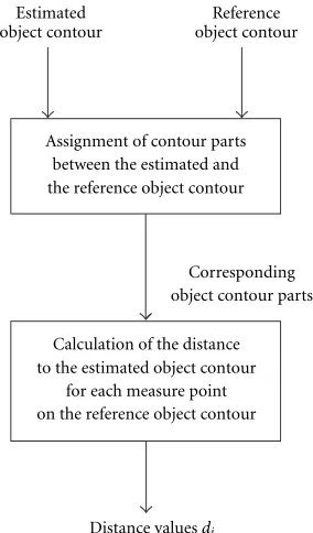
The algorithm for measuring the distance valuesdi
Estimated object contour
Reference object contour
Assignment of contour parts between the estimated and the reference object contour
Corresponding object contour parts Calculation of the distance to the estimated object contour
for each measure point on the reference object contour
Distance valuesdi
Figure1: Block diagram of the algorithm for measuring the
dis-tance valuesdibetween the reference and the estimated object
con-tour.
the reference object contour define the corresponding seg-ment in the estimated object contour (see zoomed area of Figure 2).
In the special cases that the reference object contour is in-tersected first, or the intersection point belongs to an already assigned part of the estimated object contour, the assignment is invalid (dotted arrows in Figure 2), and therefore the next pel on the reference object contour is processed. This is con-tinued until the reference object contour is not intersected as first and the resulting intersection point is not yet assigned. The segment of the estimated object contour which is sur-rounded by this intersection point and the previous intersec-tion point for which the assignment was valid (solid arrows in Figure 2) is assigned to the segment of the reference object contour, which is surrounded by the latest processed pel and the preceding pel for which the assignment was valid.
In the second step in Figure 1, the distance between cor-responding measure points on the reference and on the esti-mated object contours is calculated. A measure point is de-fined as the point on the reference or estimated object con-tour in the middle of two succeeding concon-tour pels. For each measure point on the reference object contour (rhombs in Figure 3), the average distance to all measure points within the corresponding part of the estimated object contour (cir-cles in Figure 3) is calculated. In the example, which is shown in the zoomed area of Figure 3, there are two measure points on the estimated object contour assigned to measure point 12 on the reference object contour and, therefore, two distances are calculated. These two distances are averaged, resulting in the distance valued12for the investigated measure point 12
on the reference object contour. If there is more than one measure point in the same part of the reference object
con-tour, as in the case of measure points 14 to 29 in Figure 3, the calculation is done for each of them, separately.
2.2. Temporal coherency
The temporal coherency of an estimated shape sequence is evaluated by the temporal variation of the two criteria for spatial accuracy between succeeding frames:
∆md,t=md,t−md,t−1,
∆σd,t=σd,t−σd,t−1,
(2)
wheremd,tis the normalized meanmdandσd,tis the
normal-ized standard deviationσdfor the frame at time instancet. If
the normalized meanmdand the normalized standard
devia-tionσdof the distance valuesdibetween the reference and the
estimated object contour are similar for succeeding frames, their respective temporal variation∆md,tand∆σd,tare small.
In this case the temporal coherency is judged as good. However, these two parameters do not analyze whether the measured distances keep the same value in succeeding frames, while changing their spatial position. In order to de-tect such cases, a third criterion for evaluation of the tempo-ral coherency is used, which is proposed in [8] (see Figure 4):
∆gt=
The vectorsgref
t andgestt are the gravity centers of the
eval-uated object in the reference and the estimated object mask at time instancet, respectively.∆gtis the amount of variation
from time instancet−1 totof the difference between the gravity centers in the reference and estimated object mask normalized by the maximal object expansion∅max. For this
third criterion, it is assumed that changes on the position of the estimation errors are not symmetrically distributed with respect to the gravity center.
2.3. Interpretation of results of the objective evaluation criteria
In Sections 2.1 and 2.2, criteria for evaluating the spatial ac-curacy and the temporal coherency of an estimated object shape are proposed. Furthermore, it is described how these criteria are measured. In this subsection it is discussed how these criteria can be interpreted.
For evaluation of the spatial accuracy of an estimated shape two criteria are used, the normalized meanmdand the
normalized standard deviationσdof the measured distances
di. For a specific application both criteria should be lower
than given thresholds in order to meet the demanded ac-curacy. For example, one class of applications, which would contain MPEG-4 [13] and MPEG-7 [17] content generation tools, demands a high spatial accuracy, which means low val-ues for md andσd. Another class of applications could
al-low a few shape errors, but overall the shape should be well estimated. This class, which could include tools for scene interpretation, demands mainly a small mean value md. A
Pel on estimated object contour
Pel on reference object contour
Reference object contour Estimated object contour
Valid assignment Invalid assignment
Figure2: Example for the assignment of contour parts between the estimated and the reference object contour.
Pel on estimated object contour
Pel on reference object contour
Reference object contour
Estimated object contour
Valid assignment
Measure point on reference object contour
Measure point on estimated object contour
1 2 3
4 5 6 7
8 9
10 11
12 13
14 15 16 17 18 19
20 21
22 23 24 25 26
27 28
29 12
Figure3: Example for the calculation of the distance to the estimated object contour for each measure point on the reference object contour.
advantage, if the shape has to be coded. For this class,mdcan
be larger, butσdmust be small.
Additionally, for the case that a human observer should not be disturbed by the spatial inaccuracy of an estimated shape, thresholds formd andσd can be found. This means
that it is possible to represent the impression that a human observer gets from a shape estimation result by the two pro-posed criteria for spatial accuracy, opening the door to re-placing subjective evaluation by objective criteria.
In an analogous way, the above statements are valid for the temporal evaluation criteria. For a given application, thresholds for∆md,t,∆σd,t, and∆gt have to be fixed. Then,
it can be decided if the temporal behavior of the shape esti-mation errors is good enough for a specific application.
3. EXPERIMENTAL RESULTS
The proposed evaluation method has been applied to shape estimation results for several test sequences. Thereby, a good correspondence with the visual impression of the results was established.
greft−1 gestt−1
gest t
greft
Reference object contour Estimated object contour Gravity center
Difference vector between gravity center
Figure4: Evaluation of the temporal coherency by investigating the
temporal variation of the gravity center difference (gref
t −gestt )
be-tween succeeding frames at time instancest−1 andt.
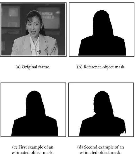
(a) Original frame. (b) Reference object mask.
(c) First example of an estimated object mask.
(d) Second example of an estimated object mask.
Figure5: Examples for 2D-shape estimation results for frame 30 of
the MPEG-4 test sequenceAkiyo.
the MPEG-4 test sequence Akiyo. The corresponding ref-erence shape represented by an object mask is shown in Figure 5b. Figures 5c and 5d present two examples for shape estimation results. The first one (Figure 5c) is the reference object mask after dilation [18], which therefore has various small estimation errors around the object contour. This cor-responds to case 1 in the introduction. In the second one (Figure 5d), which corresponds to case 2 in the introduction, a part of the left arm and a part of the hair of the person are missing. Thus, there are large estimation errors mainly
Table1
Estimation result md[%] σd[%]
Object mask in Figure 5c 0.856 0.437
Object mask in Figure 5d 0.824 1.485
Table2
Estimation result ∆md,30[%] ∆σd,30[%]
Object mask in Figure 5c 0.856 0.437
Object mask in Figure 5d 0.824 1.485
at two positions of the object contour. Although both shapes look very different, they would give similar values for the spa-tial accuracy, if evaluated by an approach from the literature, for example, [6]. Using the evaluation method proposed in this paper, the two criteria for evaluating the spatial accuracy have the values (given as percentage) in Table 1.
The normalized meanmdof the estimation errors of both
shapes is nearly equal. However, their normalized standard deviationσdis quite different. Therefore, the spatial accuracy
of both results is judged different if using the proposed eval-uation method.
Assuming that the two estimation results in Figure 5 have been perfect for the preceding frame 29, both, md andσd
would have been zero. Then, the temporal coherency crite-ria for frame 30,∆md,30and∆σd,30, would be as in Table 2.
The temporal variation of the normalized mean∆md,30
is nearly the same for both estimation results, because in the case of the mask in Figure 5c there is small temporal shape activity around the whole object, while in case of the mask in Figure 5d the temporal shape activity is much higher, but mainly at two positions of the object. However, caused by this, the temporal variation of the normalized standard de-viation∆σd,30 is small for the mask in Figure 5c and much
larger for the mask in Figure 5d. This shows that the case of several areas of small contour activity can be distinguished from the case of only a few areas, but of larger activity. There-fore, also the second problem from the introduction is solved by the proposed evaluation method.
0 10 20 30 40 50 60 70 80 90
(a) Normalized mean of distances.
0 10 20 30 40 50 60 70 80 90
(b) Normalized standard deviation of distances.
0 10 20 30 40 50 60 70 80 90
(c) Variation of normalized mean of distances.
0 10 20 30 40 50 60 70 80 90
(d) Variation of normalized standard deviation of distances.
0 10 20 30 40 50 60 70 80 90
(e) Variation of normalized gravity center difference.
Figure6: Evaluation of 2D-shape estimation results for the MPEG-4 test sequenceAkiyo(10 Hz) generated by the COST 211 Analysis Model
0 10 20 30 40 50 60 70 80 90
(a) Normalized mean of distances.
0 10 20 30 40 50 60 70 80 90
(b) Normalized standard deviation of distances.
0 10 20 30 40 50 60 70 80 90
(c) Variation of normalized mean of distances.
0 10 20 30 40 50 60 70 80 90
(d) Variation of normalized standard deviation of distances.
0 10 20 30 40 50 60 70 80 90
(e) Variation of normalized gravity center difference.
Figure7: Evaluation of 2D-shape estimation results for the MPEG-4 test sequenceHall-monitor(10 Hz) generated by the COST 211 Analysis
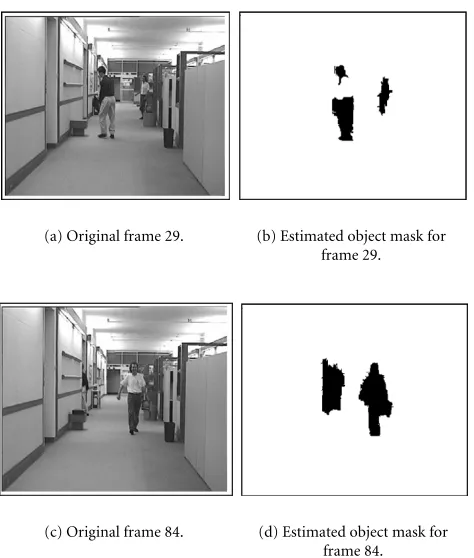
(a) Original frame 29. (b) Estimated object mask for frame 29.
(c) Original frame 84. (d) Estimated object mask for frame 84.
Figure8: 2D-shape estimation results of the COST 211 Analysis
Model (Version 5.1) for the MPEG-4 test sequenceHall-monitor
(10 Hz).
the difference between the gravity centers (Figure 6e) is not much affected by these estimation errors, because they are quite small.
Figure 7 shows the evaluation results for the test sequence Hall-monitor. Here, only the shape of the person on the left side of the image is evaluated. This person becomes visible in the second frame, but appears in the estimation result of frame 6 for the first time. Therefore, the two spatial criteria are zero for frame 0 and very large for frames 1 to 5 (Figures 7a and 7b). In the following frames the mean of the estima-tion errors lies between 2 and 15% of the object expansion. There are only two exceptions: the first one is between frames 26 and 29, where half of the body of the person is missing (see Figures 8a and 8b). The second one is between frames 80 and 84, where the person leaves the scene so that he is not visible after frame 84 (see Figures 8c and 8d). Because of the mem-ory usage in the COST 211 Analysis Model and some shadow effects in the scene, the disappearance of the person is not detected. This results in a growing estimation error, which is visible in Figure 7a. Figure 7b presents the normalized stan-dard deviation of the distances. Its value is large especially between frames 26 and 29, where half of the body is missing. This is reasonable, because in the missing part of the body the estimation errors are much larger than in the other part. Thus, the estimation errors are quite different. Of course for these frames also the temporal variation of the gravity center difference is large, as it can be seen in Figure 7e.
4. CONCLUSIONS
In this paper a method for objective evaluation of 2D-shape estimation results is proposed. The estimation error of an es-timated object shape is defined as the distance between the reference and the estimated object contour, which is mea-sured for several points of the reference object contour. For evaluating the spatial accuracy, the mean and the standard deviation of the measured distances are calculated.
It is shown that the normalized mean of the measured deviations between the estimated and the corresponding ref-erence shape is a useful criterion to evaluate the spatial accu-racy. Furthermore, by the normalized standard deviation it can be distinguished if an estimated shape has several small estimation errors or if it has only a few, but larger, estimation errors.
For evaluating the temporal coherency, the temporal variation between succeeding frames of the normalized mean and of the normalized standard deviation is investigated. It is shown that by these two criteria it can be assessed if there are various small contour activity areas around the object tour between succeeding frames, or if there is a higher con-tour activity, but only at a few positions of the object concon-tour. A third criterion is applied to detect changes of the spa-tial position of estimation errors. It evaluates the temporal variation of the difference between the gravity centers of the reference and the estimated shape.
The approach has been tested with shape estimation re-sults for several test sequences. Thereby, a good correspon-dence with the visual impression of the results was estab-lished. This have lead to use the evaluation approach within the project COST 211.
Finally, it is explained that the evaluation method can be adapted to a specific application by definition of olds for the spatial and temporal criteria. Specifically, thresh-olds can be found to model a human observer’s impression on estimation errors. Furthermore, it is possible to combine the proposed evaluation method with the ideas from [6, 8], where positive and negative distances are distinguished.
ACKNOWLEDGMENTS
This work has been partially supported by the grant CI-CYT TIC2001-0996 of the Spanish Government and by the German Fraunhofer Gesellschaft under contract no. E/E815/X5241/M0413.
REFERENCES
[1] M. Borsotti, P. Campadelli, and R. Schettini,
“Quantita-tive evaluation of color image segmentation results,” Pattern
Recognition Lett., vol. 19, no. 8, pp. 741–747, 1998.
[2] P. Correia and F. Pereira, “Estimation of video object’s
rel-evance,” inEuropean Conference on Signal Processing
(EU-SIPCO ’2000), Tampere, Finland, September 2000.
[3] P. Correia and F. Pereira, “Objective evaluation of relative
segmentation quality,” inInt. Conference on Image Processing
(ICIP), pp. 308–311, Vancouver, Canada, September 2000. [4] C. E. Eroglu and B. Sankur, “Performance evaluation
Signal Processing Conference (EUSIPCO ’2000), pp. 917–920, Tampere, Finland, September 2000.
[5] M. D. Levine and A. M. Nazif, “Dynamic measurement of
computer generated image segmentations,” IEEE Trans. on
Pattern Analysis and Machine Intelligence, vol. 7, no. 2, pp. 155–165, 1985.
[6] X. Marichal and P. Villegas, “Objective evaluation of
seg-mentation masks in video sequences,” inEuropean Conference
on Signal Processing (EUSIPCO ’2000), vol. 4, pp. 2193–2196, Tampere, Finland, September 2000.
[7] K. McKoen, R. Navarro-Prieto, B. Duc, E. Durucan, F. Ziliani, and T. Ebrahimi, “Evaluation of video segmentation methods
for surveillance applications,” inProc. European Signal
Pro-cessing Conference 2000, Tampere, Finland, September 2000. [8] P. Villegas, X. Marichal, and A. Salcedo, “Objective
evalu-ation of segmentevalu-ation masks in video sequences,” inProc.
Workshop on Image Analysis for Multimedia Interactive Services (WIAMIS ’99), pp. 85–88, Berlin, Germany, May/June 1999. [9] M. Wollborn and R. Mech, “Refined procedure for
objec-tive evaluation of VOP generation algorithms,” Doc. ISO/IEC JTC1/SC29/WG11 MPEG98/3448, Fribourg, Switzerland, Oc-tober 1997.
[10] W. A. Yasnoff, J. K. Mui, and J. W. Bacus, “Error measures
for scene segmentation,”Pattern Recognition, vol. 9, no. 4, pp.
217–231, 1977.
[11] Y. J. Zhang, “A survey on evaluation methods for image
seg-mentation,”Pattern Recognition, vol. 29, no. 8, pp. 1335–1346,
1996.
[12] Y. J. Zhang, “Evaluation and comparison of different
segmen-tation algorithms,” Pattern Recognition Lett., vol. 18, no. 10,
pp. 963–974, 1997.
[13] MPEG-4: Doc. ISO/IEC JTC1/SC29/WG11 N2502, “Informa-tion Technology—Generic Coding of Audiovisual Objects, Part 2: Visual, Final Draft of International Standard,” Octo-ber 1998.
[14] M. Gabbouj, G. Morrison, F. Alaya-Cheikh, and R. Mech, “Redundancy reduction techniques and content analysis for multimedia services—The European COST 211quat action,” inProc. Workshop on Image Analysis for Multimedia Interactive Services (WIAMIS ’99), pp. 69–72, Berlin, Germany, 31 May– 11 June 1999.
[15] B. Marcotegui, P. Correia, F. Marques, et al., “A video object
generation tool allowing friendly user interaction,” in
Interna-tional Conference on Image Processing (ICIP ’99), Kobe, Japan, October 1999.
[16] R. Mech and F. Marques, “Objective evaluation criteria for
2D-shape estimation results of moving objects,” in Proc.
Workshop on Image Analysis for Multimedia Interactive Services (WIAMIS ’01), Tampere, Finland, May 2001.
[17] MPEG-7: Doc. ISO/IEC JTC1/SC29/WG11 N2822, “Visual
Part of Experimentation Model Version 2.0,” Vancouver,
Canada, July 1999.
[18] M. Sonka, V. Hlavac, and R. Boyle,Image Processing, Analysis,
and Machine Vision, Chapman & Hall Computing, London, UK, 1993.
[19] A. Alatan, L. Onural, M. Wollborn, R. Mech, E. Tuncel, and T. Sikora, “Image sequence analysis for emerging interactive multimedia services—The European COST 211 framework,” IEEE Trans. Circuits and Systems for Video Technology, vol. 8, no. 7, pp. 802–813, 1998.
Roland Mech received the Diplom-Informatiker degree in computer science from the University of Dortmund, Dort-mund, Germany, in 1995. Since 1995 he is with the “Institut f¨ur Theoretische Nachrichtentechnik und Informationsver-arbeitung” at the University of Hannover, Germany, where he works in the areas of image sequence analysis and image
se-quence coding. He is a member of the European project COST 211. Furthermore, he was a member of the finished European project ACTS-MoMuSys and contributed actively to the ISO/MPEG-4 standardization activities. His present research interests cover image sequence analysis, especially 2D-shape estimation of moving objects, and the application of object-based image sequence coding.
Ferran Marqu´esreceived the Electrical En-gineering degree from the Polytechnic Uni-versity of Catalunya (UPC), Barcelona, Spain, in 1988. From 1989 to June 1990, he worked in the Swiss Federal Institute of Technology in Lausanne (EPFL) in the group of “Digital image sequence process-ing and codprocess-ing.” In June 1990, he joined the Department of Signal Theory and
Commu-nications of the Polytechnic University of Catalunya (UPC). From June 1991 to September 1991, he was with the Signal and Image Processing Institute at USC in Los Angeles, California. He received the Ph.D. degree from the UPC in December 1992 and the Span-ish Best Ph.D. thesis on Electrical Engineering Award-1992. Since 1995, he is Associate Professor at UPC, having served as Asso-ciate Dean for International Relations of the Telecommunication School (ETSETB) at UPC (1997–2000). He is lecturing on the area of digital signal and image processing. His current research inter-ests include still image and sequence analysis, still image and se-quence segmentation, image sese-quence coding, motion estimation and compensation, mathematical morphology and biomedical ap-plications. In the area of image coding and representation, he has been a very active partner in the MPEG-4 standard process, mainly through the European project MoMuSys. In MoMuSys, he acted as Work Package Leader of the Video Algorithms work package that, among other tasks, implemented the MPEG4 VM. He has served
as Officer responsible for the Membership Development (1994–