R E S E A R C H
Open Access
Performance of regression-based
precoding for multi-user massive MIMO-OFDM
systems
Ali Yazdan Panah
*†, Karthik Yogeeswaran
†and Yael Maguire
Abstract
We study the performance of a single-cell massive multiple-input multiple-output orthogonal frequency-division multiplexing (MIMO-OFDM) system that uses linear precoding to serve multiple users on the same time-frequency resource. To minimize overhead, the channel estimates at the base station are obtained via comb-type pilot tones during the training phase of a time-division duplexing system. Polynomial regression is used to interpolate the channel estimates within each coherence block. We show how such regressors can be designed in an offline fashion without the need to obtain channel statistics at the base station, and we assess the downlink performance over a wide range of system parameters.
Keywords: MIMO, OFDM, Massive MIMO, Least squares, Interpolation, Channel estimation, Zero-forcing, Beamforming, Precoding
1 Introduction
Multi-user multiple-input multiple-output (MU-MIMO) systems with large number of base station antennas hold the promise of high throughput communications for emerging wireless deployment [1–4]. Using the notion of
spatial multiplexing, the antenna array at the base station
can serve a multiplicity of autonomous user terminals on the same time-frequency resource. Thisspatial resource
sharing policy serves as an alternative not only to the
need for costly spectrum licensing but also the costly procurement of additional base stations in conventional cell-shrinking strategies. While the benefits of spatial mul-tiplexing may be fully realized when the number of base station antennas is equal to the number of scheduled user terminals, MU-MIMO systems with an excessively large number of antennas, also known as massive MIMO, have recently gained attention owing in part to the following benefits [5]:
*Correspondence: [email protected] †Equal contributors
Facebook Connectivity Lab, Facebook Inc., 1 Hacker Way, Menlo Park, CA 94025, USA
• Massive MIMO can increase the throughput and simultaneously improve the radiated energy efficiency via energy focusing.
• Massive MIMO can be built with rather inexpensive components by replacing high-power (W) linear amplifiers with low-power (mW) counterparts. • Massive MIMO can simplify the multiple-access
layer (MAC) by scheduling the users on the entire band without the need for feedback1.
Such benefits largely stem from asymptotic results on random matrix theory that illustrates how the effects of uncorrelated noise and small-scale fading are virtually eliminated (and the required transmitted energy per bit vanishes) as the number of antennas in a MIMO cell grows to infinity.
Massive MIMO systems are also versatile over a wide range of system parameters. For instance, the beam-forming gain afforded by using a large number of transmit antennas may be used to overcome the large path loss associated with mmWave links in urban areas [6]. Alternatively, the beamforming gain may be har-nessed at VHF/UHF frequencies to provide wide-coverage
connectivity to rural areas of the world [7]. Given such promises, the practical and theoretical aspects of mas-sive MIMO systems are actively under scrutiny for potential beyond-4G wireless communication deploy-ments not only by standardization entities such as the 3rd Generation Partnership Project (3GPP) but also by many industrial base station and device manufacturers worldwide.
Coherent massive MIMO systems require channel state information (CSI) at the base station in order to compute linear precoder filters for the downlink and equalization filters for the uplink. Such systems are typically designed for a time-division duplexing (TDD) scheme where the uplink and downlink share the transmission bandwidth. This is primarily due to the fact that the CSI may be readily obtained in TDD mode when reciprocity is main-tained in the signal path. For example, the base station may estimate the downlink (and uplink) channel using pilot symbols transmitted by the users during an uplink “training phase” [8]. The estimation of CSI is a well-studied area for MIMO [8], OFDM [9, 10], and MIMO-orthogonal frequency-division multiplexing (OFDM) [11] systems. For multi-user systems, the base station may use the estimated CSI obtained from uplink pilots to construct linear precoders (and equalizers). Fortunately, in the mas-sive MIMO regime, the performance of such filters are known to be close to the optimal schemes. In this context, matched-filter (MF) and zero-forcing (ZF) are two popu-lar linear filters [12]. The gains due to linear processing must be weighed by the increases in baseband compu-tational complexity as a result of adding more antenna elements at the base station. For instance, MF and ZF equalization are known to have linear and cubic com-plexity, respectively, in the number of users. This may present a bottleneck given current hardware capabilities; hence, some researchers have devised suboptimal meth-ods with reduced complexity such as the ordering scheme proposed in [13] for MF or the inversion-approximation for ZF proposed in [14]. The accuracy of these linear fil-ters depend on the accuracy of the CSI on which they are obtained from.
Interpolating a reduced set of pilots is a popular method of estimating the CSI across the frequency band in single and multi-user MIMO-OFDM system (see, e.g., [9, 10, 15–17] and references therein). In this paper, we study the effects ofregression-based interpolationof CSI and its effects on the accuracy of linear precoding in a downlink massive MIMO system. We propose polynomial regression as a way to interpolate the multiplexed pilots in the uplink into a single channel estimate over a block of bandwidth, i.e., over a coherence block. These regres-sors may be computed in an offline fashion without any knowledge of the channel. In Section 2, we formulate the problem and propose some notation and in Section 3, we
present numeric results. We make concluding remarks in Section 4.
Notation:Bold uppercase and lowercase letters
repre-sent matrices and vectors, respectively.X∗,XT,XH,X−1, andX+denote conjugate, transpose, conjugate-transpose, matrix inverse, and Moore-Penrose inverse of a matrixX, respectively.
2 System model
We consider a linearly precoded MU-MIMO-OFDM sys-tem over N subcarriers with M antennas at the base station servingKsingle-antenna users. The system oper-ates under a hardware-calibrated time division duplexing (TDD) scheme over a wireless channel with a coher-ence time of Tc seconds. This allows simultaneous
uplink (users to base station) and downlink (base sta-tion to users) transmissions across a common frequency band.
2.1 Uplink pilot phase (training)
During the uplink pilot phase, the users transmit pilot symbols to the base station for the purposes of chan-nel estimation and precoder/equalizer calculation. To minimize the overhead associated with pilot transmis-sions, we adopt a comb-type pilot arrangement where the pilot symbols are uniformly inserted into OFDM sym-bols during the uplink pilot phase. The pilot spacing in the frequency domain is chosen to be smaller than the coherence bandwidth of the channel which is approxi-mated asBc =0.02/τrms, whereτrmsis the channel delay
spread. As such, the channel estimation is processed on a per resource block (RB) basis, where a resource block is defined as a contiguous group of subcarriers spanning one coherence bandwidth (within the channel coherence timeTc). The pilot symbols are not precoded by the users
and are instead transmitted in a multiple-access fash-ion. Figure 1 illustrates an example of an uplink pilot resource grid over one RB spanning 12 subcarriers with a total of 24 user-transmitting pilots across 6 OFDM symbols.
2.1.1 Least squares channel estimation
The OFDM channel between each base station antenna and each user can be estimated using the uplink pilots with a least squares (LS) method. With a sufficiently long cyclic prefix (CP) length, the received signal at symbol timeton antennamat subcarriern, from thekth user, at the base station is as follows:
ym[t,n]=Cm,k[t,n]sk[t,n]+vm[t,n] , (1)
where Cm,k[t,n] is the channel frequency response,
Fig. 1Pilot tone allocation over one resource block (RB) consisting of 12 subcarriers and 6 symbols. Each user is allocated three pilot tones per RB, and this pattern is repeated over the frequency band
modulation (QAM)) pilot tone corresponding to userk, and vm[t,n] is additive white Gaussian noise (AWGN).
Since the channel is assumed constant within an RB, we re-formulate the received signal of (1) to represent the
rth RB:
y(mr)[t,n]=Cm(r,)k[t,n]s(kr)[t,n]+v(mr)[t,n] . (2)
Here,t andn denote subsets of OFDM symbols and subcarriers, respectively, in which userkhas transmitted a pilot tone within therth RB. LetLdenote the total number of pilot tones per user per RB.2For example, in Fig. 1 for user 1, we have n = {1, 5, 9},t = {1}, and for user 2, we haven = {2, 6, 10},t = {1}, and for user 24, we have
n = {4, 8, 12},t = {6}, etc. In this case, for any user, we haveL=3.
The transmitted pilot tones are chosen from the unit-energy quadrature phase shift keying (QPSK) constella-tion space so thats(kr)[t,n]2 = 1. The noise is normal distributed:v(mr)[t,n]∼ CN(0, 1) and i.i.d across m, t,
andn, and the channel response Cm(r,)k[t,n] absorbs all
link budget parameters (such as path loss and thermal noise variance). The demodulated CSI on the pilot subcar-riers for userkon RBris as follows:
Cm(r,)k[t,n]=y(mr)[t,n]s(kr)[t,n]∗. (3)
2.2 Regressive interpolation
With the channel estimated on the pilot tones, the channel at other subcarriers may be computed via interpolation. In this paper, we use a polynomial
regression-based approach formulated as a weighted
average:
Cm(r,)k[n]=
t,n
γ(r)
m,k[n,t,n]C
(r)
m,k[t,n]=γ
(r) m,k[n]c
(r) m,k,
(4)
where γ(mr),k[n] is a row vector of length L of elements γ(r)
m,k[n,t,n] which are the interpolation weights
associ-ated with antenna m for user k for the rth RB for the
nsubcarrier, for allt,n. We callγm(r),k[n] the
the valuesC(mr),k[t,n] for allt,n. The interpolation vec-tor may be computed from a polynomial regression of orderp, represented by the vectorx<mp,k>=[x0,x1,. . .,xp]T
satisfying:
Vm<p,k>xm<p,k>=c(mr),k, (5) where V<mp,k> is the L × (p+ 1) Vandermonde matrix. For 0 ≤ p < L, the solution to this linear system of equations is
x<mp,k>=
V<mp,k>
+
c(mr),k, (6)
where
V<mp,k>
+
=V<mp,k>
T
V<mp,k> −1
V<mp,k>
T
(7)
is the Moore-Penrose pseudo-inverse ofV<mp,k>. Withx<mp,k> in hand, the channel estimate at any subcarriernin the RB is simply an evaluation on the polynomial function:n0x
0+
n1x
1+n2x2+. . .+npxp. Definingd[n]=[1,n,n2,. . .,np],
in vector form, we have
Cm(r),k[n]=d[n]
V<mp,k>
+
cm(r,)k, (8) Comparing the left-hand side of (8) with (4), we see that
γ(r)
m,k[n]=d[n]
V<mp,k>
+
. (9)
Some further simplification is possible in (9) since the Vandermonde matrix and interpolation vector do not depend on the antenna indexm(as seen in Fig. 1, the pilot subcarrier locations are fixed for anym). Also, the inter-polation vector does not depend on the RB index since the pilot subcarrier location pattern is identical across RBs. For a system withNsubcarriers per RB, we have
γk[n]=d[n]
V<kp>+,n=1, 2,. . .,N (10) As a result, the interpolated CSI across all subcarriers (in any RB) in (4) can be rewritten as follows:
Cm(r),k[n]=γk[n]c(mr),k. (11) Finally, it should be noted that while suboptimal by design, the polynomial interpolation method described above may present some advantages compared to the well-known linear minimum mean square error (LMMSE) channel interpolators of [9, 10]. For example, the polyno-mial interpolators are both channel model and channel
signal-to-noise ratio (SNR) independent. Moreover, the per-RB-based processing nature of the polynomial inter-polation method may lead to computational savings since for N total subcarriers andN subcarriers per RB, the LMMSE method requires inversion of complex-valued
matrices of size NNL, while the polynomial interpolators require inversion ofreal-valuedVandermonde matrices of sizepwherep<L≤ NNL.
2.3 Downlink precoding
During the downlink phase, the base station trans-mits precoded data to the users. Let the vector s[n]=[s1[n] ,s2[n] ,. . .,sK[n] ] represent the QAM
sym-bols intended for the user terminals at subcarrier n
and v[n]∼ CN(0,IK) be AWGN at the user
ter-minals. Similar to (1), the received signal at the users may be modeled by the K × 1 vector y[n] as follows:
y[n]=C[n]F[n]s[n]+v[n] , (12)
where C[n] is the K × M downlink MIMO channel from the base station to the user terminals that absorbs the link budget parameters (such as path loss and noise variance) and also transmit power constraint of the base station. The elements of the channel matrix are estimated during the uplink pilot phase and are given by (8). F[n]= fTn,1,fTn,2,. . .,fTn,K is the M × K pre-coding matrix at subcarrier n so that fn,k is the
pre-coding vector allocated to user k by the base station for subcarrier n. We consider ZF precoding in this paper:
FZF[n]= C[n]HC[n]C[n]H
−1
, (13)
where the elements ofC[n] are obtained using polynomial regression via (11).
3 Numeric results
consists of 6 OFDM symbols with QPSK pilot symbols multiplexed for 24 users as in Fig. 1. The pilot phase is followed by DL data transmissions with QPSK sym-bols. The DL transmit powers, path loss, link budgets, and noise variance are such that the SNR for each user is identical.
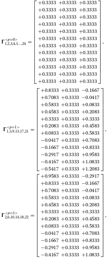
The channel frequency response estimates are computed using (8) using polynomial regressors of the order p = 0, 1, 2. The interpolation vectors
γk[n] may be computed offline and selected from
the rows of base matrices <kp>, where the sub-scripts denote the user indices corresponding to Fig. 1. We elaborate on this idea using an example below.
Example 1.In Fig. 1, for user 1, we have n =
{1, 5, 9},t = {1}, meaning there are L = 3 pilot tones per RB allocated to this user. For p = 2, the 3 × 3 Vandermonde matrix in (10) and its inverse can be com-puted as follows:
V<1p=2>=
Since each RB is defined as 12 subcarriers in Fig. 1, the length of three interpolation vectors
γ1[n] can be computed for any n = 1, 2,. . ., 12 via
(10) and the inverse Vandermonde matrix above. For example, γ1[1] and γ1[2] are computed as
=[1.0000, 0.0000, 0.0000] ,
γ1[2]=[1, 2, 4] polation vectors may be collected in the N × L base
matrix:
<p=1>
3.1 Performance vs. SNR: interpolation accuracy
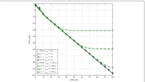
The polynomial regression orderpdetermines the inter-polation matrices used to compute the channel estimates over the frequency band. The selection of the regression order depends on (a) the quality of the channel estimates on the pilot tones, i.e., the SNR and (b) the channel vari-ability, i.e., the delay spreadτrms. It is shown in [15] that
in high channel noise, higher-order interpolation may be affected more adversely than lower-order interpolation. In Figs. 2 and 3, we confirm this observation for the proposed polynomial regressors by plotting the normalized channel estimation mean square error (NMSE) and the error vec-tor magnitude (EVM) versus SNR. We plot results for both flat fading (Rayleigh), i.e.,τrms=0, and a frequency
selec-tive channels withτrms = 0.104μs. As a baseline for the
Fig. 2NMSE versus SNR for(M,K)=(96, 24),τrms=0 (Rayleigh),τrms=0.104μs
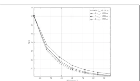
Fig. 4Downlink average SER versus SNR for(M,K)=(96, 24),τrms=0 (Rayleigh),τrms=0.104μs
methods are close to the genie-aided system, even for low-order regression models. Figure 4 shows the corre-sponding average symbol error-rate (SER) performance confirming this observation.
3.2 Performance vs.M: the massive MIMO effect
To serveKusers, the base stations need to be equipped with at leastM=Kantennas.3However, owing to larger array gain and “favorable propagation,” the performance can improve by adding more antennas to the base station. To confirm this observation, in Fig. 5, we plot the sim-ulated downlink SER versus the number of base stations antennas. The SNR is fixed at 10 dB for all the data points, and the channel delay spread isτrms=0.104μs. We
com-pare results for polynomial regression vectors of orders
p=0, 1, 2. The results show that a zero-order-hold inter-polator (p = 0) performs best and is within 6 dB of the genie-aided system whenMis large.
4 Conclusions
In this correspondence, we assessed the performance of regression-based linear precoding in the downlink of a multi-user massive MIMO-OFDM system. Simple lin-ear polynomial regressors were used to reduce multiple channel estimates over the resource blocks. These regres-sors do not depend on the channel statistics and can be computed in an offline manner. Simulations showed that for practical SNR ranges, the performance of the pro-posed methods are close to the genie-aided system, even for low-order regression selections. Moreover, the order of the regressor vectors may be adapted to the channel conditions to obtain optimal performance.
Endnotes
1This is true for time-division duplexing (TDD) where
channel reciprocity holds.
2Assumed to be equal for all users over any RB. 3Otherwise, the ZF precoder matrix in (13) does not
exist.
Competing interests
The authors declare that they have no competing interests.
Acknowledgements
The authors would like to thank members of the Connectivity Lab at Facebook for their valuable input during the course of this project.
Received: 1 July 2015 Accepted: 13 March 2016
References
1. TL Marzetta, Noncooperative cellular wireless with unlimited numbers of base station antennas. IEEE Trans. Wireless Commun.9(11), 3590–3600 (2010)
2. H Yang, TL Marzetta, Performance of conjugate and zero-forcing beamforming in large-scale antenna systems. IEEE J. Selected Areas Commun.31(31), 172–179 (2013)
3. F Rusek, D Persson, BK Lau, EG Larsson, TL Marzetta, O Edfors, F Tufvesson, Scaling up MIMO: opportunities and challenges with very large arrays. IEEE Signal Process. Mag.30(1), 40–60 (2013)
4. Y-H Nam, BL Ng, K Sayana, Y Li, J Zhang, Y Kim, J Lee, Full-dimension MIMO (FD-MIMO) for next generation cellular technology. IEEE Commun. Mag.51(6), 172–179 (2013)
5. O Edfors, F Tufvesson, Massive MIMO for next generation wireless systems. IEEE Commun. Mag.52, 187 (2014)
6. AL Swindlehurst, E Ayanoglu, P Heydari, F Capolino, Millimeter-wave massive MIMO: the next wireless revolution? IEEE Commun. Mag.52, 57 (2014)
7. H Suzuki, R Kendall, K Anderson, A Grancea, D Humphrey, J Pathikulangara, K Bengston, J Matthews, C Russell, inProceedings Int. Symp. on Commun. And Inform. Tech. (ISCIT). Highly spectrally efficient Ngara Rural Wireless Broadband Access Demonstrator (IEEE, Gold Coast QLD, 2012), pp. 914–919
8. M Biguesh, AB Gershman, Training-based MIMO channel estimation: a study of estimator tradeoffs and optimal training signals. IEEE Trans. Signal Process.54(3), 884–893 (2006)
9. S Coleri, M Ergen, A Puri, A Bahai, Channel estimation techniques based on pilot arrangement in OFDM systems. IEEE Trans. Broadcast.48(3), 223–229 (2002)
10. H Arslan, et al., Channel estimation for wireless OFDM systems. IEEE Surv. Tutorials.9(2), 18–48 (2007)
11. H Minn, N Al-Dhahir, Optimal training signals for MIMO OFDM channel estimation. IEEE Trans. Wireless Commun.5(5), 1158–1168 (2006) 12. M Vu, A Paulraj, MIMO wireless linear precoding. IEEE Signal Process. Mag.
24(5), 86–105 (2007)
13. K Alnajjar, PJ Smith, GK Woodward, et al., in2014 Communications Theory Workshop (AusCTW). Low complexity V-BLAST for massive MIMO (IEEE, Sydney, NSW, 2014), pp. 22–26
14. M Wu, B Yin, G Wang, C Dick, JR Cavallaro, C Studer, Large-scale MIMO detection for 3GPP LTE: algorithms and FPGA implementations. IEEE J. Selected Topics Signal Process.8(5), 916–929 (2014)
15. K-C Hung, DW Lin, Pilot-aided multi-carrier channel estimation via MMSE linear phase-shifted polynomial interpolation. IEEE Trans. Wireless Commun.9(8), 2539–2549 (2010)
16. X Wang, K Liu, inIEEE Global Telecommunications Conference. OFDM channel estimation based on time-frequency polynomial model of fading multi-path channels, vol. 1 (IEEE, San Antonio, TX, 2001), pp. 212–216 17. H Tang, KY Lau, RW Brodersen, inIEEE Global Telecommunications
Conference. Interpolation-based maximum likelihood channel estimation using OFDM pilot symbols, vol. 2 (IEEE, Taipei, Taiwan, 2002),
pp. 1860–1864
Submit your manuscript to a
journal and benefi t from:
7Convenient online submission 7Rigorous peer review
7Immediate publication on acceptance 7Open access: articles freely available online 7High visibility within the fi eld
7Retaining the copyright to your article