Efficient Generation of Power In Medium Voltage Direct Current Systems: Variable Speed Operation and Rectifier Considerations

(1)

University of South Carolina

Scholar Commons

Theses and Dissertations

1-1-2013

Applications of the Lopsided Lovász Local Lemma

Regarding Hypergraphs

Austin Tyler Mohr

University of South Carolina

Follow this and additional works at:https://scholarcommons.sc.edu/etd

Part of theMathematics Commons

This Open Access Dissertation is brought to you by Scholar Commons. It has been accepted for inclusion in Theses and Dissertations by an authorized administrator of Scholar Commons. For more information, please [email protected].

Recommended Citation

Mohr, A. T.(2013).Applications of the Lopsided Lovász Local Lemma Regarding Hypergraphs.(Doctoral dissertation). Retrieved from

(2)

Applications of the Lopsided Lovász Local Lemma

Regarding Hypergraphs

by

Austin Mohr

Bachelor of Science

Southern Illinois University at Carbondale, 2007

Master of Science

Southern Illinois University at Carbondale, 2008

Submitted in Partial Fulfillment of the Requirements

for the Degree of Doctor of Philosophy in

Mathematics

College of Arts and Sciences

University of South Carolina

2013

Accepted by:

László Székely, Major Professor

Joshua Cooper, Committee Member

Linyuan Lu, Committee Member

George McNulty, Committee Member

Peter Nyikos, Committee Member

Edsel Peña, External Examiner

(3)

Dedication

Dedicated to the memory of Professor Thomas D. Porter,

(4)

Acknowledgments

I give my sincere thanks to the Department of Mathematics and the Graduate School

of the University of South Carolina at Columbia, whose combined generosity made

this endeavor possible.

I am grateful to Dr. Linyuan Lu, whose expertise has touched many of the results

contained herein.

I am endlessly indebted to my advisor, Dr. László Székely. He has guided me

through this thicket with patience and skill. In so doing, he has enabled me to begin

exploring on my own.

Finally, I offer much love to my wife, Mary, who gives me courage when I have

(5)

Abstract

The Lovász local lemma is a powerful and well-studied probabilistic technique useful

in establishing the possibility of simultaneously avoiding every event in some

collec-tion. A principle limitation of the lemma’s application is that it requires most events

to be independent of one another. The lopsided local lemma relaxes the

require-ment of independence to negative dependence, which is more general but also more

difficult to identify. We will examine general classes of negative dependent events

involving maximal matchings of uniform hypergraphs, partitions of sets, and

span-ning trees of complete graphs. The results on hypergraph matchings (together with

the configuration model of Bollobás) yield asymptotically the number of regular,

uni-form hypergraphs avoiding small cycles. Finally, we work toward a characterization

of hypergraphs for which the matching paradigm is guaranteed generate negative

(6)

List of Figures

Figure 2.1 Canonical event for single-edge matching in K6. . . 15

Figure 2.2 Matchings K, L, andM, respectively. . . 16

Figure 4.1 Forest inK4 and its canonical event. . . 35

Figure 4.2 Forests D,E, and F, respectively. . . 35

Figure 5.1 Configuration projecting to 3-regular, 2-uniform multihyper-graph on four vertices. . . 43

Figure 6.1 Perfect matching host (noF as described in theorem). . . 54

Figure 6.2 Not a perfect matching host, as evidenced by red edges. . . 54

(9)

Chapter 1 The Lopsided Local Lemma

1.1 Dependency Graphs and the Local Lemma

A collection of events is avoidable whenever the probability that no event in the

collection occurs is nonzero. In the language of probability, a collection of events A1,

. . ., An is avoidable precisely when Pr

Vn

i=1Ai

>0.

Any finite collection of mutually independent events is avoidable (provided, of

course, no event occurs with probability 1); the probability of avoiding the collection

is Qn

i=1Pr

Ai

, which is greater than zero.

The requirement of mutual independence is quite stringent. We might expect the

collection can still be avoided as long as the events do not depend strongly on one

an-other. The Lovász local lemma makes this intuition precise by providing restrictions

on the interdependence of events sufficient to guarantee the possibility of avoiding

the collection. Erdős and Lovász [13] first introduced this idea to establish the

exis-tence of a certain hypergraph coloring. Subsequent generalizations culminated in the

customary version appearing, for example, in Alon and Spencer [2].

A key component in the lemma is the dependency graph, which is a simple

graph ([n], E) whose edges are situated such that the each event Ai is independent

of the event algebra generated by the collection {Aj |ij /∈E}.

The dependency graph is a convenient way to organize information about possible

dependencies among the events. For example, suppose we want to know the

(10)

edge between A1 and another event, the graph contains no information about their

relationship. If we consider a collection of non-neighbors of A1, however, the graph

tells us thatA1 is independent of the event algebra generated by the non-neighboring

events.

Trivially, a complete graph is always a dependency graph. Such a graph is useless,

however, since it contains no information about the events. At the other extreme, a

dependency graph with no edges tells us we are dealing with a collection of mutually

independent events. In practice, therefore, we hope to produce a dependency graph

that is as sparse as possible, since this tells us the collection in question is very much

like a collection of mutually independent events.

The Lovász local lemma asserts a collection is avoidable whenever there is a

corre-sponding dependency graph together with an intricate upper bound on the probability

of each individual event. In fact, it provides an explicit lower bound on the probability

of avoiding the collection. Asymmetric version (that is, one in which the probability

of every event is given the same upper bound) of the lemma was first introduced by

Erdős and Lovász [13] to address a question about hypergraph 2-colorability, which

we will discuss later. Subsequently, Spencer [26, 27] presented various generalizations

of the lemma in his work on Ramsey numbers. Presented below is a slight weakening

of the customary version appearing in Alon and Spencer [2]. (In that text, the local

lemma and the lopsided version to come are both written in terms of digraphs rather

than graphs. The topics herein will not require this additional generality.)

Lemma 1.1(Lovász Local Lemma). LetA1, . . ., Anbe events with dependency graph

([n], E). If there are numbers x1, . . . , xn ∈[0,1) such that

Pr (Ai)≤xi

Y

ij∈E

(1−xj)

for all i, then

Pr

n

^

i=1 Ai

!

≥ n

Y

i=1

(11)

1.2 2-Coloring Hypergraphs

Erdős and Lovász [13] provide an upper bound on the maximum degree of a properly

2-colorable hypergraph can contain. Their idea was to color the vertices uniformly at

random with two colors and impose conditions under which the random process would

produce a proper coloring with nonzero probability. They developed the symmetric

version of the local lemma as a tool to aid in the analysis of the resulting probability

space.

Lemma 1.2 (Lovász Local Lemma, Symmetric Version). Let A1, . . ., An be events

with dependency graph of maximum degree d. If

• Pr (Ai)≤p for all i and

• ep(d+ 1)≤1,

then

Pr

n

^

i=1 Ai

!

>0.

(The symmetric version follows from the Lemma 1.1 by setting eachxi = _d₊₁1 and

using the fact that 1− 1

d+1

d

> 1_e.)

Let H be a hypergraph in which every edge contains at least k vertices and

color the vertices uniformly at random with two colors. Our ambient probability

space will therefore contain all possible 2-colorings (both proper and improper) of

the vertices of H weighted uniformly. For each edge f ∈E(H), define the event Af

to be the collection of all 2-colorings in which the edge f is monochromatic. The

event V

f∈E(H)Af thus contains all 2-colorings in which no edge is monochromatic.

That is, it contains all proper 2-colorings. We are therefore interested in determining

when PrV

f∈E(H)Af

>0, which can be approached via the local lemma.

First, notice the events in the collection {Af | f ∈F} are mutually independent

(12)

and

E(G) ={f g |f and g share a vertex in H}

is therefore a dependency graph whose maximum degree is the same as the maximum

degree of H.

By hypothesis, every edge ofHhas at leastkvertices, so Pr (Af)≤ ₂k1−1, which we

take as our value for pin the lemma. It remains to maximize d under the constraint

ep(d+ 1)<1, which works out to d=j2k−1

e −1

k

.

Theorem 1.3. LetH be a hypergraph in which every edge contains at leastkvertices.

If H has maximum degree at most 2k_e−1 −1, then H is 2-colorable.

Before leaving this problem behind, notice we could only apply the local lemma

by ensuring that “most” events were independent. We will see later that the lopsided

local lemma can be applied in spaces where there is no independence among the

events.

1.3 Negative Dependency Graphs and the Lopsided Local Lemma

The Lovász local lemma allows us to detect avoidability if there is onlysome

indepen-dence among the events (provided we can discover a dependency graph and suitable

numbers xi). Erdős and Spencer [14] analyzed the proof and determined that one

can still detect avoidability even if there is no independence among the events.

In the following definition, let N(v) denote the set of neighbors of the vertex v

together withv itself. Anegative dependency graphfor a collection of eventsA1,

. . ., An is a simple graph ([n], E) whose edges are situated such that the inequality

Pr

 A_i

^

j∈S

Aj



≤Pr (A_i) (1.1)

holds for each i ∈ [n] and every subset S of N(i) (excluding those S for which

the event V

(13)

undefined). Stated in this way the inequality might be crudely summarized to say

that the probability of an event falls when some of its non-neighbors do not occur.

Alternative formulations of Inequality 1.1 arise from straightforward algebraic

manipulation. As before, we assume i ∈ [n] and S ⊆ N(i) are arbitrary, except

that we do not consider collections S for which the conditioning event (if any) has

probability zero. The first two are the conditional probabilities

Pr   ^ j∈S Aj Ai  ≤Pr

  ^ j∈S Aj   and

PrAi

≤Pr   ^ j∈S∪{i} Aj ^ j∈S Aj  .

Our final formulation takes the form of the correlation inequality

Pr (Ai) Pr

  _ j∈S Aj  ≤Pr

 A_i∧

_

j∈S

Aj

 .

A collection of events may satisfy the inequalities above even though no two events

are independent, as we describe in the next section.

The lopsided local lemma differs from the previous version only by replacing

“de-pendency graph” with “negative de“de-pendency graph”. Since every de“de-pendency graph

is a negative dependency graph (but not vice versa), the lopsided version is strictly

more general. It was first introduced by Erdős and Spencer [14] with regard to

Latin transversals and independently by Albert, Frieze, and Reed [1] in their work

on Hamiltonian cycles. The lemma as it appears below is due to Ku [17] and appears

as a remark in Alon and Spencer [2].

Lemma 1.4 (Lopsided Local Lemma). Let A1, . . ., An be events with negative

de-pendency graph ([n], E). If there are numbers x1, . . . , xn∈[0,1) such that

Pr (Ai)≤xi

Y

ij∈E

(1−xj)

for all i, then

Pr n ^ i=1 Ai ! ≥ n Y i=1

(14)

Proof. Take as granted for a moment that

Pr

 A_i

^ j∈S Aj 

≤x_i (1.2)

for any strict subset S of [n] and any i /∈S.

The conclusion of the lopsided local lemma follows from this claim by observing

Pr n ^ i=1 Ai !

= PrA1

·PrA2

A1

· · ·Pr

 A_n

n−1 ^ j=1 Aj   ≥ n Y i=1

(1−xi)

>0.

It remains to establish Inequality 1.2, which we accomplish by induction on |S|.

When |S| = 0, the claimed inequality reduces to Pr (Ai) ≤ xi, which is provided by

the hypotheses of the lopsided local lemma. For |S| >0, set S1 ={j ∈ S | ij ∈ E}

and S2 =S\S1. Now,

Pr

 A_i

^ j∈S Aj  =

PrAi∧Vj∈S1Aj

V

k∈S2Ak

PrV

j∈S1Aj

V

k∈S2Ak

.

We will bound the numerator and denominator separately.

For the numerator, we have

Pr

 A_i∧

^ j∈S1 Aj ^ k∈S2 Ak  ≤Pr

 A_i

^ k∈S2 Ak  

≤Pr (Ai)

≤xi

Y

j∈S1

(1−xj),

where the second inequality comes from the fact thatAi is negative dependent of the

collection {Ak |k∈S2}.

(15)

equal to 1). Now, Pr   r ^ `=1 Aj`

^ k∈S2 Ak   = Pr  Aj1

^ k∈S2 Ak  ·Pr

 Aj2

Aj1 ∧

^

k∈S2

Ak

 · · ·Pr

 Ajr

r−1 ^ `=1 Aj`∧

^ k∈S2 Ak   ≥ r Y `=1

(1−xj`),

where the inequality holds by the induction hypothesis (in each factor, we condition

on an intersection of fewer than |S|events).

Combining the two bounds,

Pr

 A_i

^ j∈S Aj  =

PrAi∧Vj∈S1Aj

V

k∈S2Ak

PrV

j∈S1Aj

V

k∈S2Ak

≤ xi

Q

j∈S1(1−xj)

Q

j∈S1(1−xj)

=xi,

which proves the claim.

1.4 Counting Derangements

A derangement is a permutation having no fixed point. It is well known that the

number of derangements on the set [N] is the integer nearest to N_e! [15]. The lopsided

local lemma gives this value as an asymptotic lower bound. (Using the forthcoming

machinery of positive dependency graphs, Lu and Székely [21] obtained this as an

asymptotic upper bound, as well.)

In the uniform probability space containing all permutations on the set [N], let

Ai denote the collection of all such permutations having i as a fixed point. The

event VN

i=1Ai contains precisely those permutations having no fixed point (that is,

(16)

No pair of distinct events Ai and Aj are independent, since

Pr (Ai∧Aj) =

(N −2)!

N! =

1 N2₋_N,

while

Pr (Ai) Pr (Aj) =

(N −1)! N! ·

(N −1)!

N! =

1 N2.

For this reason, the local lemma fails in the worst possible way. Remarkably, the

lop-sided local lemma succeeds in thebest possible way, allowing for anedgeless negative

dependency graph.

Theorem 1.5. In the uniform probability space containing all permutations on the

set [N], let Ai denote the collection of all such permutations having i as a fixed point.

The graph with vertex set [N] and no edges is a negative dependency graph for the

events {A1, . . . , AN}.

Lu and Székely [20] prove a more general statement about random injections, of

which the theorem above is a simple case. Before presenting an alternative proof, let

us take a moment to see why we might expect it to hold for just two events. Asking

whether PrA1

A2

is less than or equal to Pr (A1) can be phrased as follows: Does

the knowledge that the element 2 is not a fixed point reduce the likelihood that the

element 1 is a fixed point? The fact that 2 is not a fixed point means it is slightly

more likely than usual that it is mapped to 1, so it is slightly less likely than usual

that 1 is a fixed point.

Proof of Theorem 1.5. Without loss of generality, we will establish the inequality

Pr   k ^ j=1 Aj AN  ≤Pr

  k ^ j=1 Aj  

for any k ∈[N−1], which is defined to be

AN ∧

Vk

j=1Aj

|AN|

≤

Vk

j=1Aj

(17)

Now,AN is the collection of permutations on the set [N] havingN as a fixed point, so

|AN|= (N−1)!. Clearing denominators, we are left with establishing the inequality

N

AN ∧ k ^ j=1 Aj ≤ k ^ j=1 Aj ,

which we achieve by the following combinatorial argument.

Since all permutations belonging toAN∧Vkj=1Aj haveN as a fixed point, we may

view the event as the collection of all permutations on the set [N−1] having no fixed

points in the set [k]. The event Vk

j=1Aj is the collection of all permutations on the

set [N] also having no fixed points in the set [k]. Denote these collections by AN−1

and AN, respectively.

For any σ∈ AN−1, define σi for each i∈[N] via

σi(j) =

                  

N if j =i

σ(i) if j =N

σ(j) otherwise.

Each σi is distinct, since σi(N) =6 σj(N) whenever i 6= j. Moreover, distinct

permutations σ and τ belonging to AN−1 must differ in at least two coordinates, so

σi 6=τj for any i andj. Finally, sinceσ has no fixed points in [k], neither does σi for

any i (recall that N /∈[k]), which means each σi belongs toAN. Taken together, we

conclude N|AN−1| ≤ |AN|, as desired.

With an edgeless negative dependency graph in hand, we can take each xi = _N1

in the lopsided local lemma, since

Pr (Ai) =

1

N =xi =xi

Y

ij∈∅

(1−xj).

The lopsided local lemma concludes

Pr N ^ i=1 Ai ! ≥ N Y i=1

1− 1

N

=

1− 1

N

,

which converges to 1_e. Therefore, N_e! is an asymptotic lower bound for thenumber of

(18)

1.5 Asymptotic Enumeration with the Lopsided Local Lemma

For asymptotic analysis, we will be interested in sequences of problems in which the

size of the events and/or the ambient probability space depends on some parameter

tending toward infinity. For example, the events “at least one head” or “at least

√

N heads” in the probability space of all possible outcomes of N coin flips induce a

sequence of problems when N grows without bound. We will denote such a growing

probability space by ΩN to emphasize that its size depends on N. Lu and Székely

[21] provide conditions under which an asymptotic lower bound for PrVn

i=1Ai

can

be obtained from the lopsided local lemma. Notice Pr (Ai) will depend on N even if

the eventAi does not explicitly referenceN, since the size of the ambient probability

space ΩN grows with N.

Theorem 1.6 (Lu, Székely 2011). Let A1, . . ., An be events in a probability space

ΩN with negative dependency graph ([n], E) and set µ = Pni=1Pr (Ai). If there is (depending on N) such that

• Pr (Ai)< for all i,

• X

j:ij∈E

Pr (Aj) + 2 Pr2(Aj)< for all i, and

• µ tends to zero as N tends to infinity,

then

Pr

n

^

i=1 Ai

!

≥(1−o(1))e−µ.

Negative dependency graphs are more general but also more difficult to identify

than dependency graphs. Lu, Székely, and the author [19] exploredconflict graphs

in several disparate classes of combinatorial objects, which has been a successful

avenue in discovering negative dependency graphs. For the sake of concreteness,

(19)

matchings, set partitions, and spanning trees, which are the classes of combinatorial

objects with which we will be concerned.

To obtain an asymptotic upper bound for PrVn

i=1Ai

, Lu and Székely [21]

in-troduced the -near positive dependency graph. In the event that the lower

and upper bounds match in the limit, one obtains an asymptotic expression for the

probability of interest.

For eventsA1,. . .,Anand∈(0,1), an-near positive dependency graph ([n], E)

is one in which

• Pr(Ai∧Aj) = 0 whenever ij ∈E and

• the inequality

Pr

 A_i

^

j∈S

Aj



≥(1−) Pr(A_i)

holds for each i and any subset S of N(i) (excluding those S for which the

event V

j∈SAj has probability zero, in which case the conditional probability is

undefined).

Notice the reversal in the direction of the inequality (as compared with the

nega-tive dependency graph) results in an upper bound on PrVn

i=1Ai

.

Theorem 1.7 (Lu, Székely 2011). If A1, . . ., An are events with an -near positive

dependency graph, then

Pr

n

^

i=1 Ai

!

≤ n

Y

i=1

[1−(1−) Pr (Ai)].

With some extra restrictions, this upper bound meets the lower bound in 1.6

asymptotically.

Corollary 1.8. Let A1, . . ., An be events with an -near positive dependency graph

in a probability space growing with N and set µ = Pn

(20)

Pn

i=1Pr 2₍_A

i) tend to zero as N tends to infinity, then

Pr n ^ i=1 Ai !

≤(1 +o(1))e−µ.

Proof. Theorem 1.7 gives

Pr n ^ i=1 Ai ! ≤ n Y i=1

[1−(1−) Pr (Ai)]

= exp

n

X

i=1

log [1−(1−) Pr (Ai)]

!

.

Using the fact that

log(1−x) = − ∞

X

k=1 xk

k

for |x|<1, we write

log [1−(1−) Pr (Ai)] =− ∞

X

k=1

(1−)k_Prk

(Ai)

k

for each i. Now,

− n X i=1 ∞ X k=1

(1−)kPrk(Ai)

k =−

n

X

i=1

(1−) Pr(Ai)− n X i=1 ∞ X k=2

(1−)kPrk(Ai)

k

=− n

X

i=1

(1−) Pr(Ai)− n

X

i=1

OPr2(Ai)

=− n

X

i=1

(1−) Pr(Ai)−O n

X

i=1

Pr2(Ai)

!

.

Substituting into the exponential, we have

Pr n ^ i=1 Ai ! ≤exp n X i=1

log [1−(1−) Pr (Ai)]

!

= exp − n

X

i=1

(1−) Pr(Ai)−O n

X

i=1

Pr2(Ai)

!!

= exp (−µ) exp µ+O

n

X

i=1

Pr2(Ai)

!!

(21)

In a sequence of problems satisfying the conditions of both Theorem 1.6 and

Corollary 1.8, we can conclude PrVn

i=1Ai

is asymptotic to e−µ. If we further

assume that the ambient probability space is equipped with the counting measure,

then multiplying by the size of the space gives an asymptotic expression for the

number of outcomes avoiding the events A1, . . ., An.

Corollary 1.9. LetA1, . . ., An be events in a uniform probability spaceΩN equipped

with the counting measure and setµ=Pn

i=1Pr (Ai). If the conditions of both Theorem

1.6 and Corollary 1.8 are satisfied, then

n

\

i=1 Ai

(22)

Chapter 2 Lopsided Local Lemma for Hypergraph

Matchings

2.1 Introduction

Ans-matching(or simply matching) in ans-uniform hypergraph is a collection of

vertex-disjoint edges (each containingsvertices) and ismaximalprovided no strictly

larger matching contains it. Let Ω denote the uniform probability space consisting

of all maximal matchings of some underlyings-uniform hypergraph H. Our primary

objective in this section will be to define a conflict graph for events in Ω (analogous

to the one defined in Chapter 3 for set partitions) and present some conditions under

which it is a negative dependency graph.

For a particular matchingM, defineAM to be the collection of all maximal

match-ings extending M. More precisely,

AM ={L∈Ω|M ⊆L}.

We call the collection AM the canonical event for the matching M to emphasize

its interpretation as an event in the probability space Ω. Two matchings conflict

whenever their union is not again a matching, and two canonical events conflict when

the matchings used to define them conflict.

Finally, let M be any collection of s-matchings. The conflict graph for the

collection {AM |M ∈ M} of canonical events is a simple graph whose vertex set is

(23)

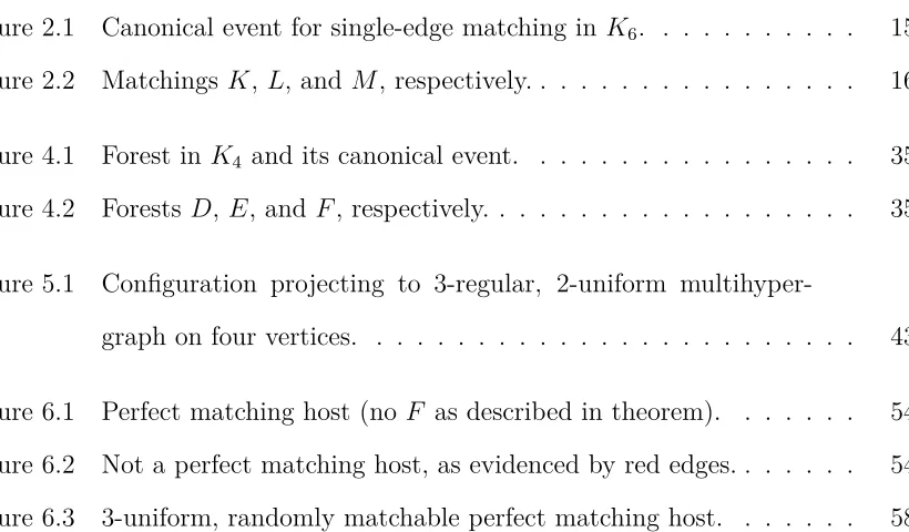
Figure 2.1 Canonical event for single-edge matching in K6.

2.2 Example Conflict Graph

Take the complete graph on six vertices to be the underlying graph (a graph is a

2-uniform hypergraph). The single-edge matchingB is pictured in Figure 2.2 together

with its canonical event AB, which consists of the three maximal (indeed, perfect)

matchings containing the edge B. The edges incident to a vertex of B are not

pic-tured to emphasize the fact that they cannot possibly be including in any matching

containing B. For this reason, there is a natural bijection between the outcomes of

the canonical eventAB and the collection of perfect matchings of the complete graph

on four vertices.

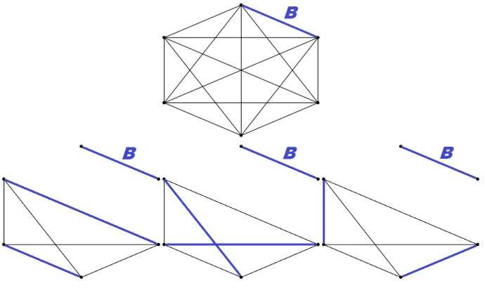
Unrelated to the previous example, consider the three matchings K, L, and M

in the complete graph on six vertices pictured in Figure 2.2. The matchings K

and M conflict, because their union is not again a matching. The canonical events

(not pictured) AK and AM are disjoint, since no perfect matching extends both the

matchingsK andM simultaneously. Similarly, the matchingsLandM conflict. The

matchings K and L do not conflict, since their union is itself a matching (indeed, a

(24)

Figure 2.2 Matchings K, L, and M, respectively.

vertex set{K, L, M} and edge set {KM, LM}.

2.3 Negative Dependency Graph

For the enumeration of regular uniform hypergraphs in Chapter 5, the underlying

graph will be a complete uniform hypergraph, in which case the conflict graph is

always a negative dependency graph [19].

Theorem 2.1 (Lu, M, Székely 2012). Let M be any collection of matchings in a

complete uniform hypergraph. The conflict graph for the collection {AM | M ∈ M}

of canonical events is a negative dependency graph.

At this point our interest in hypergraph matchings is two-fold. In Chapter 5, we

apply the theorem above (together with other tools) to the asymptotic enumeration

of regular uniform hypergraphs. In Chapter 6, we pursue the classification of the

underlying hypergraphs for which the theorem above holds.

2.4 Positive Dependency Graph

Let M be a collection of matchings in the complete s-uniform hypergraph on N

vertices with negative dependency graph (M, E), and letδ be a positive real number.

(For the moment, we may suppose that sand δ are both fixed, but later applications

(25)

no matching from M is a subset of another matching from M and the following

inequalities are satisfied for every matching M ∈ M and every edgee∈E:

• Pr (AM)< δ

• X

L:LM∈E

Pr (AL) + Pr2(AL)< δ

• X

L:e∈L

Pr (AL) + Pr2(AL)< δ

• X

L∈MM

Pr

N−s|M|(AL) + Pr

2

N−s|M|(AL)< δ,

where

MM ={L\M |L∈ M, L=6 M, L∩M 6=∅, Ldoes not conflict with M}.

A collection in which every matching contains at most k edges isk-bounded.

Theorem 2.2. Let M be a collection of matchings in a complete s-uniform

hyper-graph. If M is δ-sparse and k-bounded, then the conflict graph for the canonical

events {AM |M ∈ M} is also an -near positive dependency graph.

The precise relationship between the parameters k, s, δ, and is deferred to

Section A.2.

2.5 Asymptotics for Avoiding Matchings

Let ΩN be the uniform probability space of maximal matchings of a complete uniform

hypergraph. In this space, the expression PrV

M∈MAM

denotes the probability that

a maximal matching chosen uniformly at random from ΩN contains no submatching

belonging to the set M. According to Theorem 2.1, the conflict graph for any

col-lection of canonical matching events is a negative dependency graph. Theorem 2.2

gives some restrictions onMunder which we are assured the conflict graph is also a

(26)

ensure nice asymptotic behavior. We gather here all these conditions into one place

to derive an asymptotic expression for PrV

M∈MAM

. Take note that expressions

such as Pr (AM) will depend onN since the size of the ambient probability space ΩN

depends on N.

Theorem 2.3. Let ΩN denote the uniform probability space of perfect matchings of

Ks

N, the complete s-uniform hypergraph on N vertices. Let r and both depend on

N, where r is a positive integer and is a real number eventually lying in the interval

(0,₁₆1 ). Let M be a k-bounded collection of matchings in Ks

N in which no matching

is a subset of another. For any matching M ∈ M, define the canonical event

AM ={L∈ΩN |M ⊆L}.

Set µ =P

M∈MPr (AM). Finally, suppose the following inequalities are satisfied for

every matching M ∈ M and every edge e of Ks

N:

• Pr (AM)<

• X

L:L,Mconflict

Pr (AL)<

• X

L∈M:e∈L

Pr (AL)<

• X

L∈MM

Pr

N−sk(AL)<

If, in addition, ks=o(1), then

Pr ^

M∈M

AM

!

=e−µ+O(ksµ). (2.1)

Furthermore, if ksµ=o(1), then

Pr ^

M∈M

AM

!

= (1 +O(ksµ))e−µ.

The proof (like the statement) is technical, and we relegate it to Section A.2. We

will make use of this result in Chapter 5, wherein we establish a bijection between a

(27)

Chapter 3 Negative Dependency Graphs for Set Partitions

Let Ω denote the uniform probability space consisting of all partitions of some

un-derlying set X. (Equivalently stated, Ω contains all perfect matchings of complete

nonuniform hypergraph on the vertex set X in which edges of the matching are not

required to have the same size.) Our primary objective in this section will be to define

a certain type of conflict graph for events in Ω and present some conditions under

which it is a negative dependency graph.

3.1 Introduction

A partial partition is a collection of disjoint subsets of the underlying set X. (A

partial partition may in fact fully partition the set X.) For a particular partial

partition P, define AP to be the collection of all (ordinary) partitions extending P.

More precisely,

AP ={Q∈Ω|P ⊆Q}.

(We are using the ordinary subset relation, not the refinement relation.) We call

the collection AP the canonical event for the partial partition P to emphasize its

interpretation as an event in the probability space Ω. Two partial partitionsconflict

whenever their union is not again a partial partition, and two canonical events conflict

when the partitions used to define them conflict.

Finally, let P be any collection of partial partitions of the set X. The conflict

graph for the collection {AP | P ∈ P} of canonical events is a simple graph whose

(28)

Table 3.1 Partial partitions of [5] and corresponding canonical events.

Partial Partition Canonical Event

P 12|3 AP

12|3|45 12|3|4|5

Q 14|2 AQ

14|2|35 14|2|3|5 R 12|45 AR 12|3|45

In this section we are concerned with characterizing the collections {AP |P ∈ P}

of canonical events for which the conflict graph is a negative dependency graph. In

other words, for what collections P of partial partitions does the inequality

Pr

 A_P

^

AQ∈S

AQ



 ≤Pr (A_P)

hold for each P ∈ P and every subset S of N(P)? (In this instance, N(P) is the

subset of P containing precisely those partial partitions that do not conflict with P.)

Consider the underlying set X = [5] and the partial partitions P, Q, and R defined

in Table 3.2. (The notation, for example, 12|3 is shorthand for {{1,2},{3}}.)

The partial partitions P and Q conflict, since P ∪Q = 12 | 3 | 14 | 2 is not a

collection of disjoint subsets. Notice the canonical events AP and AQ are disjoint.

Similarly, the partial partitions Q and R conflict. On the other hand, the partial

partitionsP andRdo not conflict, sinceP∪R = 12|3|45 is itself a partial partition

(in fact, it is an ordinary partition). The conflict graph for the associated canonical

events is therefore the graph with vertex set {P, Q, R} and edge set{P Q, QR}.

3.3 A Class of Counterexamples

For convenience, let us henceforth assume that the underlying set of the partitions is

[N], write ΩN to denote the space of all partitions of [N], and write Pr

(29)

the probability is taken with respect to the space ΩN.

The conflict graph need not be a negative dependency graph for arbitrary

collec-tions P of partial partitions. Indeed, a counterexample exists for every N, but the

construction presented there seems to rely on the fact that each partial partition is

quite large with respect to the underlying set. To present the counterexamples, we

introduce Nth Bell number BN [4, 5, 24], which is the number of partitions of an

N-element set.

Let the size N of the underlying set be given. For eachi∈[N], let Pi denote the

partition of [N]\ {i} into singletons. We have

Pr

N N

^

i=1 APi

! = Pr N   N _ i=1 APi

 =

BN −1

BN

,

since the only partition extending any of thePi is the partition of [N] into singletons.

On the other hand, the partition of [N + 1] into singletons extends any of the Pi.

Each Pi is also extended by the partition containing only singletons except for the

block {i, N + 1}. Thus we have,

Pr

N+1

N

^

i=1 APi

! = Pr N+1   N _ i=1 APi

 =

BN+1−(N + 1) BN+1

.

Before proceeding, we will need the fact that

Pr

N N

^

i=1 APi

! > Pr N+1 N ^ i=1 APi

!

.

Begin with the fact that (N + 1)BN > BN+1 for all integers N (see Appendix B).

Now,

(N + 1)BN > BN+1

−BN+1 >−(N + 1)BN

BN+1BN −BN+1 > BN+1BN −(N + 1)BN

BN −1

BN

> BN+1−(N+ 1) BN+1

Pr

N N

^

i=1 APi

! > Pr N+1 N ^ i=1 APi

!

(30)

as desired.

Introduce now another partial partition P ={{N + 1}}. We have

Pr

N+1

N

^

i=1 APi

AP

!

= Pr

N N

^

i=1 APi

!

> Pr

N+1

N

^

i=1 APi

!

,

violating the condition of negative dependence. Thus, the conflict graph for the events

AP,AP1,. . ., APN is not a negative dependency graph in the space ΩN+1.

3.4 Results

For a collection P of partitions of [N], leta(P) denote the average number of blocks

among the partitions belonging to P. That is,

a(P) =

P

P∈P|P|

|P| .

For example, it is known that a(ΩN) = B_BN+1

N −1 (see Appendix B). The conflict graph is a negative dependency graph for collections P that are “coarse” enough in

the sense that the average number of blocks of its corresponding canonical events is

smaller than the average over all partitions.

The following lemma will be useful for establishing negative dependency graphs

in collections of coarse partial partitions. Notice the conclusion is for the entire

collection P of partial partitions and says nothing aboutsubcollections.

Lemma 3.1. Let P be a collection of partial partitions of [N]. If

a \

P∈P

AP

!

≥ BN+1

BN −1

or, equivalently,

a [

P∈P

AP

!

≤ BN+1

(31)

then Pr N ^ P∈P AP ! ≤ Pr N+1 ^ P∈P AP ! .

Proof. For convenience, let PN ₌ T

P∈PANP and PN+1 =

T

P∈PANP+1, where the

superscript denotes the size of the underlying set. Given any partition P ∈ PN_{, one}

can form a partition belonging to PN+1 _{either by adjoining the block} _{_N _{+ 1}_} _to_P

or by introducing the element N+ 1 to any existing block of P. From this we see

P N+1 ≥ X

P∈PN

(|P|+ 1)

= P

N +

X

P∈PN |P|

= 1 +

P

P∈PN|P| |PN_|

! P N

=1 +aPN P

N

≥

1 + BN+1 BN −1 P N

=BN+1Pr

PN

,

so PrPN+1_≥_Pr_PN_.

A heavy-handed way to ensure sufficient coarseness is to require every block

ap-pearing in P be large enough. It turns out a block size of logN is large enough, and

empirical data suggests this is as small as possible. The proof of this fact relies on

Canfield’s formulation [9] of Moser and Wyman’s asymptotic expression for the Bell

numbers [23].

Lemma 3.2(Canfield 1995).Letrbe the unique real solution of the equationrer₌_N

(that is, r = LambertW0(N)). The identity

BN+h =

(N +h)! rN+h ·

exp (er−1) (2πB)1/2 ·

1 + P0+hP1+h 2_P

2

er +

Q0+hQ1+h2Q2+h3Q3+h4Q4

e2r +O(e

−3r₎

(32)

holds uniformly for h=O(logN) as N tends to infinity, where

B = (r2+r)er,

P0 =−

2r4+ 9r3 + 16r2+ 6r+ 2 24r(r+ 1)3 ,

P1 =−

r2+ 3r+ 1 2r(r+ 1)2 ,

P2 =− 1 2r(r+ 1),

Q0 =

4 + 24r+ 100r2−636r3−588r4−384r5 −143r6−12r7+ 4r8 1152r2₍_r_{+ 1)}6 ,

Q1 =

6 + 32r+ 56r2+ 135r3+ 101r4+ 37r5+ 6r6 48r2₍_r_{+ 1)}5 ,

Q2 =

20 + 90r+ 190r2_{+ 105}_r3 _{+ 20}_r4 48r2₍_r_{+ 1)}4 ,

Q3 =

5 + 15r+ 5r2 12r2₍_r_{+ 1)}3 , and

Q4 =

1 8r2₍_r_{+ 1)}2.

The factor of r = LambertW(N) proves troublesome in the asymptotic analysis,

so we make use of the following bounds [16].

Lemma 3.3 (Hoorfar, Hassani 2008). For every x≥e, we have

logx−log logx+ 1 2

log logx

logx ≤LambertW(x)≤logx−log logx+ e e−1

log logx logx

with equality only for x=e.

Lemma 3.4. Set k=dlogNe and let cbe any constant. The inequality

BN+1 BN

− BN+1−c`

BN−c`

>1

holds for all sufficiently large N and any `≥k.

Proof. The case ` = k is handled by a Maple worksheet [22] making use of the

Moser-Wyman expansion of the Bell numbers and the Hoorfar-Hassani bound on the

LambertW function. The sequence BN+1−c`

BN−c` is nonincreasing in` [12], which gives the

(33)

Theorem 3.5. Set k = dlogNe and let c be any constant. If P is a collection

(possibly depending on N) of partial partitions of a sufficiently large set [N]such that

every partial partition P ∈ P contains at most c blocks and every block contains at

least k elements, then the conflict graph for {AP | P ∈ P} is a negative dependency

graph.

Proof. LetP ∈ P and let Qbe any subcollection ofP that does not conflict withP.

Our ultimate goal is to establish

Pr

N

 

^

Q∈Q

AQ

AP

 ≤Pr

N

 

^

Q∈Q

AQ



. (3.1)

To that end, define QP = {Q\P | Q∈ Q}. Let kPk denote the number of ground

elements(not blocks) appearing in the partial partitionP and assume, without loss of

generality, that these elements areN−kPk+1,. . .,N. SinceP does not conflict with

Q, any block of P is either identical to or disjoint from any block of Q∈ Q. Hence,

the ground elements appearing in partial partitions belonging to QP are elements of

the set [N− kPk].

Now, if∅ ∈ QP, then there is nothing to show (the lefthand side of Inequality 3.1

evaluates to zero). Otherwise, let{cQP |QP ∈ QP}be nonnegative weights such that

X

QP∈QP

cQP = 1

and

a

 

[

QP∈QP

AQP

 =

X

QP∈QP

cQPa(AQP).

Fix an arbitrary partial partition QP ∈ QP and denote its blocks by B1, . . ., Bj.

Each of the Bi contains at least k elements. In what follows, we use a superscript

N on a collection of partial partitions to denote the number of ground elements over

(34)

monotonicity of the sequence BN+1 BN give

aAN_Q

P

=j +aΩN−kQPk N−kQPk

=j −1 + BN+1−kQPk

BN−kQPk

< j−2 + BN+1−kQP\{B1}k

BN−kQP\{B1}k

< j−3 + BN+1−kQP\{B1,B2}k

BN−kQP\{B1,B2}k

.. .

< j−(j + 1) +BN+1−kQP\{B1,...,Bj}k

BN−kQP\{B1,...,Bj}k

= BN+1 BN

−1.

for all sufficiently large N.

As QP was selected arbitrarily from QP, we can write

a

 

[

QP∈QP

AQP

 =

X

QP∈QP

cQPa(AQP)

< X

QP∈QP

cQP

_B

N+1 BN

−1

= BN+1 BN

−1.

(35)

of Lemma 3.1 gives Pr N   ^ Q∈Q AQ AP 

= Pr

N−kPk

 

^

QP∈QP

AQP

 

≤ Pr

N+1−kPk

 

^

QP∈QP

AQP

 

≤ Pr

N+2−kPk

 

^

QP∈QP

AQP

  .. . ≤Pr N   ^

QP∈QP

AQP

  ≤Pr N   ^ Q∈Q AQ  .

3.5 Failed Attempt via Injection

Let M be a partial partition and M be a collection of partial partitions that does

not conflict with M. The correlation inequality presented in Section 1.3 would ask

us to verify

Pr (AM) Pr

_

L∈M

AL

!

≤Pr AM ∧

_

L∈M

AL

!!

,

which is equivalent to

|AM|

[ L∈M AL

≤BN

AM ∩

[ L∈M AL ! .

A radically different approach to verifying this inequality would be to establish an

injection f from the set

(

(P, Q)|P ∈AM, Q∈

[

L∈M

AL

)

(which has cardinality equal to the left-hand side) into a set of cardinality no larger

(36)

where it comes short of achieving the desired goal. Notice that the inequality cannot

possibly be verified in full generality, since there are counterexamples for everyN. It

is the author’s hope that a similar approach can be made to work for appropriately

restricted collections of partial partitions.

Given a partial partition R, let supp(R) denote the collection of all ground

el-ements appearing in R. When speaking of the restriction of a partial partition to

another, we may write R S to mean R supp(S). Empty blocks arising as a result of

restriction are discarded.

Let C = [N]\supp(M) (“C” for “complement”). We will say a block B of a

partial partition is

• atype M block wheneverB M=B [N],

• atype C block wheneverB C=B [N], and

• amixed block if it is neither type M nor type C.

In other words, if we first restrict our attention only to elements of [N] (there

will be other kinds of elements to consider later), then type M blocks contain only

elements ofM, type C blocks contain no elements ofM, and mixed blocks contain a

mixture of the two kinds of elements.

Let now P ∈AM and Q∈SL∈M be given and let (P, Q)7→(P0, Q0) underf.

To obtain P0 fromP:

1. Remove all type M blocks from P. (Since P ∈AM, this is justP \M.)

2. Insert all type M blocks of Q into P.

3. For each mixed type block B of Q, let `B = min(B C) and insert into P the

block (B M)∪ {`c_B}, where `c_B denotes a duplicate, but distinguishable, copy

(37)

For the purposes of the function f, duplicate elements will always correspond to

elements of C, so we define Cb = {`b| ` ∈ C} as the collection of possible duplicate

elements.

To obtain Q0 fromQ:

1. Remove all type M blocks from Q.

2. Replace each mixed type block B of Q with B C.

3. Insert all blocks of M into Q.

(As an example of the behavior of f, consider M = 1|23, P = 1|23|4|56, andQ=

13|26|45. The procedure described above gives P0 = 13|2b6|4|56 andQ0 = 1|23|45|6.)

Lemma 3.6. The function f is injective.

Proof. Let f(P1, Q1) = (P10, Q

0

1) = (P

0

2, Q

0

2) = f(P2, Q2). We show (P1, Q1) =

(P2, Q2).

Since P₁0 =P₂0, it follows that P₁0 C=P20 C, and so

P1 =P10 C ∪M

=P₁0 C ∪M

=P2.

Since Q0₁ = Q0₂, it follows that Q0₁ \M = Q0₂ \M, and so Q1 C= Q2 C. Now,

every type M block of P₁0 =P₂0 is also present in bothQ1 andQ2. Every mixed block

B of P₁0 =P₂0 contains an element `b∈ Cb, and so there is B₁ ∈Q₁ and B₂ ∈Q₂ such

that` belongs to bothB1 andB2 andB1 M=B2 M=B\ {`b}. SinceQ₁ _C=Q₂ _C,

we know also that B1 C= B2 C, and thus B1 = B2. As this holds for all mixed

blocks of P₁0 =P₂0, we have Q1 =Q2.

It remains to verify the inequality

|AM|

[

L∈M

AL

≤BN

AM ∩

[

L∈M

AL

!

(38)

Since f is injective, we have

(

(P, Q)|P ∈AM, Q∈

[

L∈M

AL

)

≤

(

f((P, Q))|P ∈AM, Q∈

[

L∈M

AL

)

.

Observe that, if (P, Q)7→(P0, Q0) underf, thenQ0 ∈AM ∩(SL∈MAL), sinceM

does not conflict with M. Hence, there are at most |AM ∩(SL∈MAL)| possible Q0.

The desired inequality would follow by showing, for each fixedQ0₀ ∈AM∩(SL∈MAL),

we have

|{P0 |(P0, Q₀0)∈im(f)}| ≤BN.

Unfortunately, this inequality is not true. Fixing Q0₀ only restricts what elements

of Cb can be applied as labels in a P0 under f. The available labels are precisely the

minimum elements of typeC blocks ofQ0₀. Since Q0₀ can have as many as N−1 type

C blocks, the fact that Q0₀ is fixed can be of little help.

For a concrete example, let M = {{1}}, M contain only the partial partition

{{2}}, and Q0₀ be a partition of [N] into singletons. The partition P ∈ AM may be

any partition having the singleton block {1}. The partition Q ∈ A{{2}} that would

map toQ0₀ underf may be the partition of [N] into singletons or any partition that is

singletons except for the block{1, i}fori /∈ {1,2}. IfQis of the former type, then the

resulting P0 may be any partition having the singleton block {1}, of which there are

BN−1 possibilities. IfQis of the latter type, thenP0 may be any partition containing

the block{1,bi}for i6= 2, of which there are (N−2)B_N−₁ possibilities. In total, this

gives (N −1)BN−1 possible P0 that may appear with Q00 under f. Since

BN−1

BN ∼

r N

(wherer is the solution to the equationN =rer_{) [11], we have} (N−1)BN−1

BN ∼r, which

grows without bound in N. Hence,

|{P0 |(P0, Q₀0)∈im(f)}|> BN

(39)

3.6 Further Research

In light of the class of counterexamples in Chapter B, one cannot guarantee even

asymptotically that the conflict graph for an unrestricted collection {AP | P ∈ P}

of canonical events is a negative dependency graph. The known counterexamples

seem to rely on the fact that the set of ground elements of partial partitions in the

collectionP is quite a large subset of [N]. Empirical evidence suggests that a negative

dependency graph always exists when this is not the case.

Conjecture 3.7. LetP be a collection of partial partitions of [N0]. For sufficiently

large N, the conflict graph for {AP |P ∈ P} is a negative dependency graph in the

probability space ΩN.

While possibly true, this conjecture carries with it the unfortunate restriction that

only members of ΩN whose support lies in [N0] can be forbidden via the lopsided local

lemma.

In Chapter 5, we make use of the lopsided local lemma to derive asymptotics

for the number of hypergraphs avoiding small cycles. It was the author’s intent to

derive a similar expression for the number of partitions avoiding small blocks. For

this application, we are interested only in the collection P defined by

P ={{B}:B ⊂[N],|B| ≤m}

for some fixed (or perhaps slowly growing) integerm. Showing that the conflict graph

for this collection is a negative dependency graph would be an important step toward

proving the following conjecture about partitions having no small blocks.

Conjecture 3.8. The number of partitions of [N] whose smallest block is of size m

is asymptotic to

BNexp − m−1

X

k=1 N

k

!

BN−k

BN

!

(40)

The conjecture is correct whenm= 2, for which it claims the number of

singleton-free partitions of [N] is asymptotic to BNexp

−NBN−1 BN

. The number of such

par-titions can be expressed exactly as PN

i=1(−1)N

−i_B

i using Lemma B.2. Dividing both

sides by BN, we show _B1_N PNi=1(−1)

N−i_B

i and exp

−NBN−1 BN

converge to the same

value. For both calculations, we make use of Canfield’s expansion for the Bell

num-bers.

For the former,

1 BN

N

X

i=1

(−1)N−iBi =

BN−1 BN

N

X

i=1

(−1)N−i Bi BN−1

!

= BN−1 BN

1 +O BN−2 BN−1

!!

= BN−1 BN

1 +O

_r

n

= r

n(1 +o(1)).

For the latter,

exp

−NBN−1 BN

= exp

 −r·

1

1 + poly(_err)

 

= exp −r 1−O poly(r) er

!!!

,

since 1

1±x ∼1∓x as x→0. Continuing,

exp −r 1−O poly(r) er

!!!

= exp −r+O poly(r) er

!!

= exp (−r) exp O poly(r) er

!!

= r

(41)

Chapter 4 Negative Dependency Graphs for

Spanning Trees

The probability spaces we defined for hypergraph matchings and set partitions have

in common that a partial object (partial matching and partial partition,

respec-tively) does not conflict with any maximal object (maximal matching and partition,

respectively) in its corresponding canonical event. This useful property lends itself

immediately to the use of induction, since every maximal object splits nicely into the

partial object and its extension. The proofs presented on hypergraph matchings rely

on the fact that we can extend a partial matching M to a maximal one by taking

the disjoint union of M together with any maximal matching of the vertices missed

by M. Similarly, we extend a partial partition P to a full partition by taking the

disjoint union of P together with any partition of the ground elements missed by P.

In this section, we define a natural space in which a partial object (forest) conflicts

with every maximal object (spanning tree) in its canonical event. As a result, the

maximal objects do not split nicely into the disjoint union of a partial object together

with its extension.

4.1 Introduction

A cycle in a simple graph is a sequence of vertices and edges v1, e1, v2, e2, . . ., vk,

ek (k ≥3) in whichei ={vi, vi+1} for eachi (where we understandvk+1 to be v1). A

(42)

component of a forest is a tree.) Given an underlying graph G, we say a tree T is a

spanning treeof Gwhenever the vertex set ofT coincides with the vertex set ofG.

Let Ω be the uniform probability space containing all spanning trees of KN, the

complete graph on N vertices. For any forest F contained in KN, define the

canon-ical event AF to be the collection of all spanning trees of KN containing F. That

is,

AF ={T ∈Ω|F ⊆T}.

Two forests F1 and F2 (both contained in KN) conflict whenever there are trees

T1 ⊆F1 and T2 ⊆F2 such that T1 and T2 are neither identical nor disjoint.

Finally, let F be any collection of forests contained in KN. Theconflict graph

for the collection{AF |F ∈ F }is a simple graph whose vertex set isF. Two forests

are adjacent in this graph if and only if they conflict.

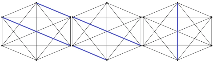
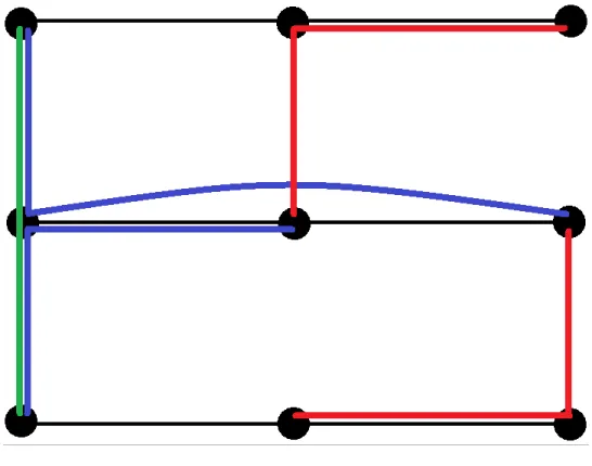
Take K4, the complete graph on four vertices, to be the underlying graph. Figure

4.2 depicts a forest contained in K4 composed of two disjoint edges. The canonical

event for this forest consists of the four spanning trees of K4 that contain it as a

subgraph. Notice every spanning tree in the canonical event conflicts with the forest

that defined it.

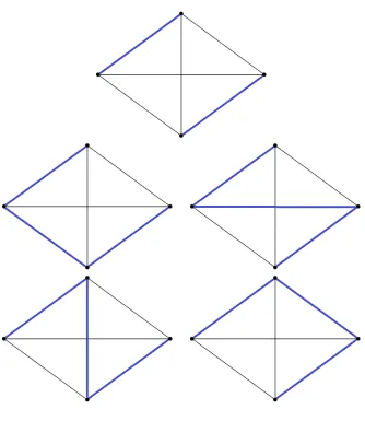
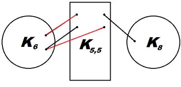
Unrelated to the previous example, consider the three forestsD,E, andF pictured

in Figure 4.2 withK8as the underlying graph. The forestsDandF conflict, since the

leftmost component ofDis neither identical to nor disjoint from the single component

ofF. Similarly, the forestsE andF conflict in the lower component ofE. The forests

D and E do not conflict, since any two components (one from D and one from E)

are either identical or disjoint. The conflict graph for the associated canonical events

(43)

Figure 4.1 Forest inK4 and its canonical event.

Efficient Generation of Power In Medium Voltage Direct Current Systems: Variable Speed Operation and Rectifier Considerations

University of South Carolina

Scholar Commons

Applications of the Lopsided Lovász Local Lemma

Regarding Hypergraphs

Austin Tyler Mohr

Dedication

Acknowledgments

Abstract

Table of Contents

List of Figures

Chapter 1

The Lopsided Local Lemma

Chapter 2

Lopsided Local Lemma for Hypergraph

Matchings

Chapter 3

Negative Dependency Graphs for Set Partitions

Chapter 4

Negative Dependency Graphs for

Spanning Trees