Medical Image Indexing using Attributed Relational Graphs and Rectangular Trees

(1)

!

"

#"#

$ % %#

&

'

((( )

Medical Image Indexing using Attributed Relational Graphs and Rectangular Trees

Sujatha Sivakumar

Abstract:Given a collection of medical images (like CT scans), we derive appropriate representations of their content and organize the images together with representations in a multi-dimensional data structure so that we can search efficiently for images similar to an example image. Image content is represented by Attributed Relational Graphs (ARGs) holding features of objects and relationships between objects. Our proposed image indexing and similarity search methods rely on the assumption that a fixed number of “labelled” or “expected” objects (e.g., “heart”, “lungs” etc) are common in all images of a given application domain in addition to a variable number of “unexpected” or “unlabeled” objects (e.g., “tumor”, “hematoma” etc). Our method can answer queries by example such as “find all X-rays that are similar to Smith’s X-ray.” The stored images are mapped to points in a multi-dimensional space and are indexed using state-of-the-art database methods (R-trees). The proposed method has several desirable properties: (a) Database search is approximate so that all images up to a pre-specified degree of similarity (tolerance) are retrieved; (b) it has no “false dismissals” (i.e. all images qualifying query selection criteria are retrieved) and (c) it is much faster than sequential scanning for searching in the main memory and on the disk (i.e. by up to an order of magnitude); thus, scaling-up well for larger databases.

Keywords:Indexing, Similarity Searching, Medical Images, R-tree, Attributed Relational Graphs

I. INTRODUCTION

In many applications, images comprise vast majority of acquired and processed data. For example, in remote sensing and astronomy, large amounts of image data are received daily by land stations for processing, analysis and archiving. A similar need for processing, analysis and archiving of images has been identified in applications such as cartography (images are analog or digitized maps) and meteorology (images are meteorological maps). The medical imaging field, in particular, has grown substantially in recent years and has generated additional interest in methods and tools for the management, analysis, and communication of medical images. Picture Archiving and Communication Systems (PACS) are currently used in many medical centers to manage the image data produced by computed tomography (CT), magnetic resonance (MRI), digital subtraction angiography (DSA), digital radiography, ultrasound, and other diagnostic imaging modalities which are available and routinely used to support clinical decision making. It is important to extend the capabilities of techniques used in such application fields by developing database systems supporting the automated archiving and retrieval of images by content.

An “Image Database” (IDB) is a “system in which a large amount of image data is stored in an integrated fashion” [1]. Image data may include: the raw images themselves, attributes (e.g., dates, names), text (e.g., diagnosis related text), information extracted from images by automated or computer assisted image analysis etc. The effectiveness of an IDB system, which supports the archiving and retrieval of images by content, ultimately depends on the types and correctness of image representations used, the types of image queries allowed, and the efficiency of search techniques implemented. In selecting an appropriate type of

image representation, an attempt must be made to reduce the dependence on the application domain as much as possible and to ensure certain level of tolerance to uncertainty with regard to image content. Furthermore, image representations must be compact to minimize storage space, while image processing, analysis and search procedures must be computationally efficient in order to meet the efficiency requirements of many IDB applications. Query response times and the size of the answer set depend highly on query type, specificity, complexity, and amount of on-line image analysis required and the size of the search. In addition, query formulation ought to be iterative and flexible, thus enabling a gradual resolution of user uncertainty. All images (and/or information related to images) satisfying the query selection criteria are retrieved and displayed for viewing.

The retrieval capabilities of an IDB must be embedded in its query language. Command oriented query languages allow the user to issue queries by conditional statements involving various image attributes (values of attributes and/or ranges of such values). Other types of image queries include: queries by identifier (a unique key is specified), region queries (an image region is specified and all intersecting regions are returned), text queries etc. The highest complexity of image queries is encountered in queries by example. In this case, a sample image or sketch is provided and the system must analyze it, extract an appropriate description and representation of its content and match this representation against representations of images stored in the database. Such queries are easy to be expressed and formulated, since the user need not be familiar with the syntax of any special purpose image query language.

(2)

of an IDB system supporting the archiving and retrieval of images by content can be significantly enhanced by incorporating efficient techniques supporting the indexing of images by content into the IDB storage and search mechanisms.

Our contribution in this paper is as follows: Given a collection of images we derive appropriate representations of their content and organize the images together with their representations in the database so that, we can search efficiently for images similar to an example image. Given a collection of medical images, each image has been segmented (automatically or manually) into closed contours corresponding to dominant image objects or regions. These are objects common in all mages of a given application domain. For example, in medical images, the expected objects may correspond to the usual anatomical structures (e.g., “heart”, “lungs”) and the outline contour of the body. All expected objects are identified prior to storage and a class or name is assigned to each one. The labeled objects need not be similar in all images. Not all objects need to be identified: Images may also contain “unexpected” or “unlabeled” objects. These may be objects not present in all images. For example, in medical images, the unexpected objects may correspond to abnormal pathological structures (e.g., “hematoma”, “tumor” etc.). The user can specify a desirable image (e.g., “find the examinations which are similar to Smith’s examination”). The system will return all the images below a distance threshold or the most similar images. For two images to be similar they must contain similar objects (regions in general) in similar spatial relationships. Our primary goal is to swiftly respond to the queries. A secondary goal is to support visualization and data mining (e.g., study of the clustering properties of the set of images).

The rest of the paper is organized as follows: In Section 2, we discuss existing methods on image retrievals. Section 3 provides a brief overview of the proposed work. Section 4 presents a detailed system analysis of our proposed methods for digital medical image indexing using the Attributed Relational Graphs (ARGs) and Rectangular trees (R-trees). Section 5 concludes the paper.

II. EXISTING METHODS ON IMAGE INDEXING, SEARCHING AND RETRIEVAL

A. Image Retrieval by Content

Image content can be described indirectly through attributes (e.g., subject, speaker, etc.) or text (e.g., captions). Queries by image content require that, prior to storage, images are processed, and appropriate descriptions of their content are extracted and stored in the database. Retrievals by image content is not an exact process (two images are rarely identical). Instead, all images with up to a pre-specified degree of similarity have to be retrieved [1]. The design of appropriate image similarity/distance functions is a key issue and is application-dependent. An almost orthogonal issue is speed of search. In this section, we review techniques for exact and approximate database search along with methods to accelerate the search.

B. Exact Match Searching in Image Databases

2-D strings [2] constitute an efficient image content representation and provide low complexity (i.e., polynomial) matching in image databases. A unique name or class is assigned to each object. The relative positions between all objects are then represented by two one-dimensional strings. The problem of image retrieval is transformed into one of string matching: All 2-D strings containing the 2-D string of the query as a substring are retrieved. Methods for speed up of retrievals based indexing of 2-D strings in a database have been proposed [3, 4]. 2-D strings [5] deal with situations of overlapping objects with complex shapes. 2-D strings may yield “false alarms” (non-qualifying images) and “false dismissals” (qualifying but not retrieved images).

C. Approximate Searching in Image Databases – No

Indexing

Systems described in the literature on Machine Vision typically focus on the quality of the features and the matching function, with little or no emphasis on the speed of retrieval. Thus, each image is described by a set of features; to respond to a query, the system searches the features of all the images sequentially. A typical, recent system supports the segmentation and interactive retrieval of facial images from an IDB [6]. A-priori knowledge regarding the kind and the positioning of expected image objects (e.g., face outline, nose, eyes etc.) is employed and used to guide the segmentation of face images into disjoint regions corresponding to the above objects. The database search is exhaustive, using sequential scanning.

D. Approximate Searching in Image Databases – with

Indexing neighbor queries efficiently. The original paper did not address the issue of false dismissals as well as the problem of retrieving images by specifying properties of objects and relationships between objects. In all of the above methods, one or more of the following drawbacks exist: (a) they do not index on the relationships between objects; (b) they do not scale up, for large, disk-based databases; (c) they have false dismissals. Our proposed method solves all these three issues.

E. Spatial Access Methods

(3)

“spatial-join”) queries. For clarity, in this paper, we focus on range queries only.

Several spatial access methods have been proposed, forming the following classes: (a) Methods that transform rectangles into points in a higher dimensionality space [8]; (b) Methods that use linear quad-trees or, equivalently, the “z-ordering” [9] or other “space filling curves” and finally (c) Methods based on trees (k-dimensional trees etc). One of the most characteristic approaches in the last class is the R-tree. The R-tree can be envisioned as an extension of the B-tree for multidimensional objects. A geometric object is represented by its Minimum Bounding Rectangle (MBR). Non-leaf nodes contain entries of the form (ptr, R) where ptr

is a pointer to a child node in the R-tree; R is the MBR that covers all rectangles in the child node. Leaf nodes contain entries of the form (object_ id, R) where object_id is a pointer to the object description, and R is the MBR of the object. The main idea behind the R-tree [10] is that father nodes are allowed to overlap. This way, the R-tree can guarantee good space utilization and remains balanced. Extensions, variations and improvements to the original R-tree structure include the packed R-R-trees, the R+-tree, the R* -tree, and the Hilbert R-tree.

III. OUR PROPOSED METHOD

Our method maps each image to a point in an f-dimensional space. The mapping of Attributed Relational Graphs (ARGs) to f-dimensional points is achieved through FastMap [11]. Similarly, queries are mapped to points in the above f-dimensional space and the problem of IDB search is transformed into one of spatial search. To speed-up retrievals, the f-dimensional points are indexed using an R-tree. Below we discuss each one of the above processing steps separately.

A. Image Segmentation

All images are segmented into closed contours corresponding to dominant image objects or regions. However, image segmentation and labeling of the components are outside the scope of this paper. We assume that each image has been segmented manually (e.g., by tracing the contours of the regions of interest). Figure 1 shows an example of an original MRI image and its segmented form. The contribution of our work is with regards to fast searching after the images and the queries have been segmented.

Figure 1. Example of an Original Gray-level Image (left) and its Segmented Form (right)

B. ARG Representation

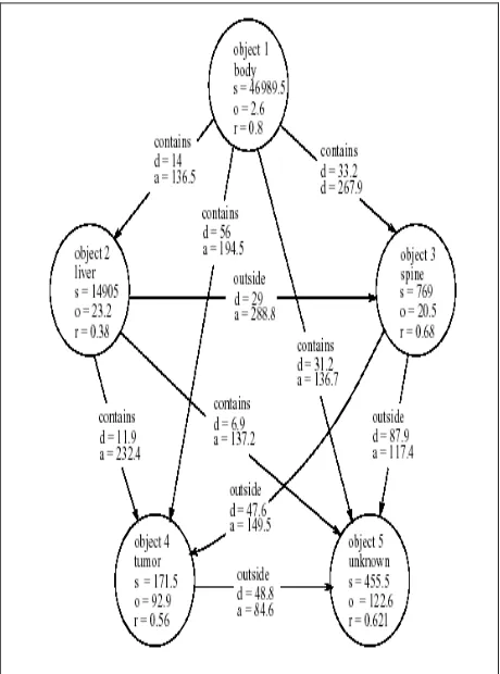
Figure 2 shows the proposed ARG representation for medical MRI images of the abdomen such as the example image of Figure 1. Nodes correspond to regions and arcs correspond to relationships between regions. Both nodes and arcs are labeled by the attribute values of the region properties and the relationship properties, respectively. Angles are in degrees. In this work, we used the following set of features: Individual regions are described by 3 attributes, namely: (i) Size ( ), computed as the size of the area of a region; (ii) Roundness ( ), computed as the ratio of the smallest to the largest second moment and (iii)

Orientation ( ), defined as the angle between the horizontal direction and the axis of elongation. This is the axis of least second moment. Spatial Relationships between regions are described by 2 attributes, namely: (i) Distance ( ), computed as the minimum distance between their contours; (ii)

Relative Angle ( ), defined as the angle with the horizontal direction of the line connecting the centers of mass of the two regions.

It is straightforward to add more features as region or relationship attributes. Additional features that could be used include the average grey-level and texture values, moments or Fourier coefficients etc. as region descriptors; relative size, amount of overlapping or adjacency etc. can be also used to characterize the relationships between regions. In any case, our proposed method can handle any set of features. However, we have strong reasons to use the above set of features. The features we used are very successful.

(4)

C. Mapping ARGs to f-dimensional Points

The FastMap algorithm accepts as input: ARGs, the Eucledian distance function and, the desired number of dimensions, and maps the above ARGs to points in an f-dimensional space. As mentioned earlier, the complexity of this mapping is f-distance computations. Each image is mapped to exactly one point.

D. Indexing – File Structure

Figure 3 demonstrates the proposed file structure of the data on the disk. Specifically, the file structure consists of the following parts:

Figure 3. File Structure

The spatial access method, holding an f-dimensional vector for each stored image (ARG). We used R-trees solely because of availability; any spatial access method would be applicable, like, e.g., R*-trees and X-trees. In fact, a faster spatial access method would only make our approach work even faster!

The “ARG file”. This is a file holding the ARGs. Each record in this file consists of (a) An identifier (e.g., the image file name) corresponding to the image from which the ARG has been derived and (b) The features of each region together with its relationships with the other regions.

The “Image store” holding the original image files. For faster display, we have also kept the segmented forms of all images.

E. Search Strategy

The user specifies a query image and a tolerance, and asks for all the images within that tolerance. The ARG of the query is computed first. Then, the f-dimensional vector of the above ARG is derived. All vectors within tolerance are retrieved from the R-tree. The R-tree may return false alarms (i.e., not qualifying images). A post-processing step is required to clean-up the false alarms. For the R-tree search, we issue a range query on the R-tree to obtain a list of promising images (image identifiers). The clean-up procedure for each of the above obtained images retrieves its corresponding ARG from the ARG file and computes the actual distance between this ARG and the ARG of the query. If the distance is less than the threshold, the image is included in the response set.

IV. SYSTEM ANALYSIS

All images are segmented into closed contours corresponding to dominant image objects or regions. Tools like Adobe Photoshop can be used for manual segmentation of images.

A. ARG Representation

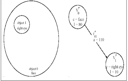
Image descriptions are given in terms of object properties and in terms of relationships between objects. The textbook approach to capture this information is the Attributed Relational Graphs (ARGs). In an ARG, the objects are represented by graph nodes and the relationships between objects are represented by arcs between such nodes. Both nodes and arcs are labeled by attributes corresponding to properties (features) of objects and relationships respectively. Figure 4 shows an example image (a line drawing showing a face) containing four objects (numbered 0 through 3) and its corresponding ARG.

Figure 4. Example Image showing a Sketch of a Face (left) and its corresponding ARG (right)

The relationship between any two objects has (in this example) also one attribute, namely, the angle (a) with the horizontal direction of the line connecting the centers of mass of these objects. The specific features which are used in the ARGs are derived from the raw image data and depending on the application, can be geometric (i.e., independent of pixel values), statistical or textural, or features specified in some transform domain (e.g., Fourier coefficients of object shapes). In the case of medical CT and MRI images used in this work, the set of features is given below.

The following properties are used to describe the individual regions of objects

Size (s), computed as the size of the area it occupies.

Roundness (r), computed as the ratio of the smallest to the largest second moment.

Orientation (o), defined to be the angle between the horizontal direction and the axis of elongation. This is the axis of least second moment.

The following properties are used to describe the spatial relationships between two objects

(5)

Relative Position (p), defined as the angle with the horizontal direction of the line connecting the centers of mass of the two objects.

However, the proposed methodology is independent of any specific kind of features. The problem of retrieving images which are similar to a given example image is transformed into a problem of searching a database of stored ARGs: Given a query, its ARG has to be computed and compared with all stored ARGs.

In comparisons between ARGs, we need a measure of the “goodness” of matching. A measure of goodness is defined here. Let Q be a query image consisting of q objects and S matching associated nodes while, the second term is the cost of matching the relationships between such nodes. In our setting, only a subset of the objects in the stored image set S

needs to be matched. There is no cost if the data image contains extra objects; however, we assume that the cost is infinite if the data image is missing one of the objects of the query. COST is the cost of matching features of objects or features of relationships between associated objects. The distance between images Q and S is defined as the minimum distance computed over all possible mappings F( ):

Dist(Q, S) = minF { DistF(Q, S) } …(2) associated to objects in Q in the same order. Then, Equation 1 can be written as follows:

DistF(Q, S) = Distp,F(Q, S) = [ k |qi - si|p ]1/p …(3) i=1

p is the order of the metric. For p = 1and p = 2, we obtain the Manhattan (city-block) and the Euclidean distance respectively. For example, the Manhattan distance between the query image of Figure 5 and the example image of Figure 4 is Dist(Q, S) = |100-80| + |15-10| - |130-110| = 45. We have omitted the subscript F because there is only one mapping. Similarity searching in an IDB of stored ARGs requires that all images within distance t must be retrieved. Specifically, we have to retrieve all the images of S that satisfy the following condition. Without loss of generality, we use the Euclidean distance (p = 2). However, the proposed method can handle any Lp metric.

Dist(Q, S) t …(4)

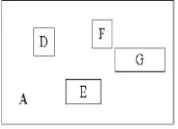
Figure 5. Matching between the Query and the Original Example Image

B. FastMap

FastMap [11] is an algorithm that takes in N ARGs, the ARG distance function and f, the desired number of dimensions, and maps the above ARGs to N points in an f-dimensional space such that distances are preserved. The goal is to solve the problem for the ‘distance case, that is, to find N points in k-dimensional space, whose Euclidian distances will match the distances of a given N x N distance matrix. The key idea is to pretend that objects are indeed points in some unknown, n-dimensional space, and to try to project these points on k mutually orthogonal directions. The challenge is to compute these projections from the distance matrix only, since it is the only input we have. For the rest of this discussion, an object will be treated as if it were a point in an n-dimensional space, (with unknown n). The main focus of the proposed method is to project the objects on a carefully selected ‘line’. To do that, we choose two objects Oa and Ob (referred to as ‘pivot objects’ from now on), and consider the ‘line’ that passes through them in n -dimensional space. The projections of the objects on that line are computed using the cosine law.

C. Indexing

Each of the f-dimensional vectors for the stored image is arranged into an indexing structure called R-Tree. One of the huge demands in geo-data applications is to respond very quickly to spatial queries. Spatial data objects often cover areas in multi-dimensional spaces. Multi-dimensional queries prevent from using classical indexing structures, for instance the B-Tree. The reason is that the database uses one-dimensional indexing structures. However, in modern information processing like CAD (Computer Aided Design), cartography and multimedia applications use multi-dimensional data objects which mean that the objects have more attributes. Thus, the database system needs an efficient multi-dimensional index structure. A number of structures have been proposed for handling multi-dimensional point data. We choose to use the R-trees (Rectangular trees), a dynamic-index data structure [10] for spatial searching and can be used to represent data objects by intervals in several dimensions.

D. R-Tree Index Structure

(6)

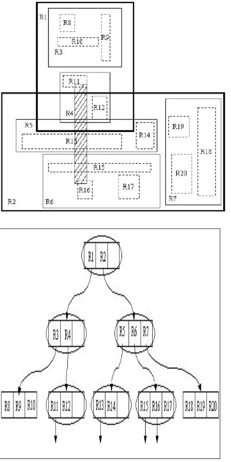
MBRs. This structure continues up to the root. Eventually the root comprises a MBR over all objects. Figure 6 shows an example of a simple R-Tree.

In Figure 6, nodes A, B and C are the root nodes. Node A, for instance, covers child nodes D, E, F and G, and contains them with a minimal bounding rectangle. An R-Tree satisfies the following properties:

1. Every leaf node contains between m and M index records unless it is the root Thus, the root can have less entries than m.

2. For each index record in a leaf node, I is the smallest rectangle that spatially contains the n-dimensional data object represented by the indicated tuple.

3. Every non-leaf node has between m and M children unless it is the root.

4. For each entry in a non-leaf node, i is the smallest rectangle that spatially contains the rectangles in the child node.

5. The root node has at least two children unless it is a leaf node.

6. All leaves appear on the same level. That means the tree is balanced.

Figure 6. Structure of a simple R-Tree

1) Structure of a Leaf Node: Leaf nodes in an R-Tree contain index record entries of the form (I, tuple-identifier) where tuple-identifier refers to a tuple in the database and I

is an n-dimensional rectangle which is the bounding box of the spatial object indexed.

I = (I0, I1, …, In-1 )

Here n is the number of dimensions and Ii is a closed bounded interval [a, b] describing the extension of the object along dimension i.

2) Structure of a Non-leaf Node: The nodes which are not leaf nodes contain entries of the form (I, child-pointer) where child-pointer is the address of a lower node in the R-Tree and I covers all rectangles in the child node's entries.

Figure 7. Root Node A covers Child Node Entries D, E, F and G

3) Maximum and Minimum Entries: Variable M is the maximum of entries which is usually given and m is the minimum of entries in one node. The minimum number of entries in a node is dependent on M with (M/2) m. The maximum number of nodes is

N

/

m

+

N

/

m

2

+

1

. Here N stands for the number of index records of the R-Tree. Variable m is jointly responsible for the height of an R-Tree and the speed of the algorithm. The choice of M

depends on the hardware, especially on hard disk properties such as capacity and sector size. If nodes have more than 3 or 4 entries, the tree is very wide, and almost all the space is used for leaf nodes containing index records.

4) Searching: The search algorithm is similar to that of the B-Tree. It returns all qualifying records which the search rectangle overlaps. The algorithm descends the tree from the root. In the same time, the algorithm checks the rectangle overlapping in the node with the searched rectangle. If the test is positive, the search just descends to the found overlapping nodes. This procedure is repeated until the leaf node. If the entries of the leaf node overlap the searched rectangle then we return these entries as a qualifying record. In Figure 8, there is a filled rectangle which is the search rectangle. The algorithm is looking for qualifying records in the filled area. The filled rectangle overlaps the root entries R1 and R2, so the algorithm checks these entries. In R1, there is just R4 which overlaps the filled rectangle. Its entries are also checked. The algorithm arrives at the leaf node level. The entries of the leaf node are checked for qualifying records. R11 is the only one and so a first search result. In R2, there are two rectangle overlaps with the filled rectangle: R5 and R6. Both of them are checked and the algorithm recognizes that at the leaf node level, the entries R13, R15 and R16 overlap with the search rectangle. Finally, the search result is R11, R13, R15 and R16.

(7)

Figure 8. Searching in an R-tree

Figure 9: Example to Illustrate the Insertion of a new Rectangle

Figure 10. Example to Illustrate the Procedure to Choose Leaf Nodes

(8)

Figure 11. Example to Illustrate the Splitting and Insertion of a Node

7) Kinds of Splits: In the case of adding a new entry to a full node containing M entries, it is necessary to divide the collection of M + 1 entries between two nodes. Insertion and Deletion have to use this method to save the tree structure. The division should be done in a way that makes it as unlikely as possible that both new nodes will need to be checked on subsequent searches. The total area of the two covering rectangles after a split should be minimized. Figure 12 shows a 'good' split and a 'bad' split. There are three versions of algorithms for SplitNode. They are: (a) Exhaustive algorithm; (b) Quadratic-cost algorithm; (c) Linear-cost algorithm.

Figure 12. Kinds of Splits: Bad Split (Left) and Good Split (Right)

Exhaustive Algorithm is normally not used. It is the best split algorithm in quality because it finds the best way to minimize the area of all rectangles of the R-Tree. The cost, however, would be 2M-1 and so the algorithm would be too slow with a large node size. Linear-cost algorithms produce the poorest quality. Hence, we use the quadratic-cost algorithm, explained below:

The quadratic-cost algorithm tries (cost: O(M2)) to find a small-area split; however, it is not guaranteed that it finds one with the smallest area possible. Quadratic-Cost algorithm chooses two of the M+1 entries, which use most of the area and puts them in new nodes. Considering the remaining entries, the entry that needs the largest area is selected, if it is inserted in one of the two nodes. The algorithm then puts the selected entry in that node where fewer enlargements are needed. The procedure is repeated until all nodes are divided or one node has less then m

entries.

V. CONCLUSIONS AND FUTURE WORK

Our proposed indexing method allows similarity search to be performed on both labeled and unlabeled (i.e., not identified) objects. Indexing is performed by decomposing each input image into sets of objects, called “sub-images”, containing all labeled objects and a fixed number of unlabeled objects. All sub-images are mapped to points in a multi-dimensional feature space and are stored in an R-tree. Image database search is then transformed into spatial search. Our proposed method outperforms sequential scanning significantly for searching in the main memory or on the disk, never missing a hit (i.e., no false dismissals). The method can accommodate any set of attributes that the domain expert will provide. With respect to future work, a very promising direction is the study of data mining algorithms on the point-transformed set of images to detect regularities and patterns, as well as to detect correlations with demographic data. Another promising direction is the use of more recent indexing structures, such as the X-Tree or the SR-Tree, which provide faster search times for smaller space overhead.

VI. ACKNOWLEDGMENTS

The corresponding author (Natarajan Meghanathan) of this paper conducts research in the areas of Computational Biology and Bioinformatics as a Senior Personnel under the U.S. National Science Foundation (NSF)-funded Mississippi EPSCoR grant (EPS-0556308) on Modeling and Simulation of Complex Systems. The views and conclusions contained in this document are those of the authors and should not be interpreted as necessarily representing the official policies, either expressed or implied, of the funding agency.

VII. REFERENCES

[1] E. G. M. Petrakis and C. Faloustos, “Similarity Searching in Medical Image Databases,” IEEE Transactions on Knowledge and Data Engineering, vol. 9, no. 3, pp. 435-477, May-June 1997. Methodology for the Representation, Indexing, and Retrieval of Images by Content,” Image and Vision Computing, vol. 11, no. 8, pp. 504-521, October 1993. [4] E. G. M. Petrakis and S. C. Orphanoudakis, “A

Generalized Approach for Image Indexing and Retrieval Based on 2-D Strings,” Intelligent Image Database Systems, pp. 197-218, World Scientific Publishing Co., 1996.

[5] S-Y. Lee and F-H. Hsu, “2-D C-String: A New Spatial Knowledge Representation for Image Database Systems,” Pattern Recognition, vol. 23, no. 10, pp. 1077-1087, 1990.

[6] J. R. Bach, S. Paul and R. Jain, “A Visual Information Management System for the Interactive Retrieval of Faces,” IEEE Transactions on Knowledge and Data Engineering, vol. 5, no. 4, pp. 619-627, August 1993. [7] H. V. Jagadish, “A Retrieval Technique for Similar

(9)

[8] J. Nievergelt, H. Hinterberger and K. C. Sevcik, “The Grid File: An Adaptable, Symmetric Multi-key File Structure,” ACM Transactions on Database Systems, vol. 9, pp. 38-71, 1984.

[9] J. A. Orenstein, “Spatial Query Processing in an Object-Oriented Database System,” Proceedings of the ACM SIGMOD International Conference on Management of Data, vol. 15, no. 2, pp. 326-336, June 1986.

[10] A. Guttaman, “R-Trees: A Dynamic Index Structure for Spatial Searching,” Proceedings of the ACM SIGMOD

International Conference on Management and Data, vol. 14, no. 2, pp. 47-57, June 1984.