Discovering E-commerce Sequential Data Sets and Sequential Patterns for Recommendation

University of Windsor University of Windsor

Scholarship at UWindsor

Scholarship at UWindsor

Electronic Theses and Dissertations Theses, Dissertations, and Major Papers

2019

Discovering E-commerce Sequential Data Sets and Sequential

Discovering E-commerce Sequential Data Sets and Sequential

Patterns for Recommendation

Patterns for Recommendation

Raj Bhatta

University of Windsor

Follow this and additional works at: https://scholar.uwindsor.ca/etd

Recommended Citation Recommended Citation

Bhatta, Raj, "Discovering E-commerce Sequential Data Sets and Sequential Patterns for Recommendation" (2019). Electronic Theses and Dissertations. 7686.

https://scholar.uwindsor.ca/etd/7686

This online database contains the full-text of PhD dissertations and Masters’ theses of University of Windsor students from 1954 forward. These documents are made available for personal study and research purposes only, in accordance with the Canadian Copyright Act and the Creative Commons license—CC BY-NC-ND (Attribution, Non-Commercial, No Derivative Works). Under this license, works must always be attributed to the copyright holder (original author), cannot be used for any commercial purposes, and may not be altered. Any other use would require the permission of the copyright holder. Students may inquire about withdrawing their dissertation and/or thesis from this database. For additional inquiries, please contact the repository administrator via email

Discovering E-commerce Sequential Data Sets and Sequential Patterns for Recommendation By

Raj Bhatta

A Thesis

Submitted to the Faculty of Graduate Studies through the School of Computer Science in Partial Fulfillment of the Requirements for

the Degree of Master of Science at the University of Windsor

Windsor, Ontario, Canada

2019

Discovering E-commerce Sequential Data Sets and Sequential Patterns for Recommendation By

Raj Bhatta

APPROVED BY:

A. Sarker

Department of Mathematics & Statistics

S. Saad

School of Computer Science

C. Ezeife, Advisor School of Computer Science

iii

DECLARATION OF ORIGINALITY

I hereby certify that I am the sole author of this thesis and part of this thesis has been submitted to Big Data Analytics and Knowledge Discovery-DAWAK19 for publication.

I certify that, to the best of my knowledge, my thesis does not infringe upon anyone’s copyright nor violate any proprietary rights and that any ideas, techniques, quotations, or any other material from the work of other people included in my thesis, published or otherwise, are fully acknowledged in accordance with the standard referencing practices. Furthermore, to the extent that I have included copyrighted material that surpasses the bounds of fair dealing within the meaning of the Canada Copyright Act, I certify that I have obtained a written permission from the copyright owner(s) to include such material(s) in my thesis and have included copies of such copyright clearances to my appendix.

iv

ABSTRACT

In E-commerce recommendation system accuracy will be improved if more complex sequential patterns of user purchase behavior are learned and included in its user-item matrix input, to make it more informative before collaborative filtering. Existing recommendation systems that use mining techniques with some sequences are those referred to as LiuRec09, ChoiRec12, SuChenRec15, and HPCRec18. LiuRec09 system clusters users with similar clickstream sequence data, then uses association rule mining and segmentation based collaborative filtering to select Top-N neighbors from the cluster to which a target user belongs. ChoiRec12 derives a user’s rating for an item as the percentage of the user’s total number of purchases the user’s item purchase constitutes. SuChenRec15system is based on clickstream sequence similarity using frequency of purchases of items, duration of time spent and clickstream path. HPCRec18 used historical item purchase frequency, consequential bond between clicks and purchases of items to enrich the user-item matrix qualitatively and quantitatively. None of these systems integrates sequential patterns of customer clicks or purchases to capture more complex sequential purchase behavior.

This thesis proposes an algorithm called HSPRec (Historical Sequential Pattern Recommendation System), which first generates an E-Commerce sequential database from historical purchase data using another new algorithm SHOD (Sequential Historical Periodic Database Generation). Then, thesis mines frequent sequential purchase patterns before using these mined sequential patterns with consequential bonds between clicks and purchases to (i) improve the user-item matrix quantitatively, (ii) used historical purchase frequencies to further enrich ratings qualitatively. Thirdly, the improved matrix is used as input to collaborative filtering algorithm for better recommendations. Experimental results with mean absolute error, precision and recall show that the proposed sequential pattern mining-based recommendation system, HSPRec provides more accurate recommendations than the tested existing systems.

v

DEDICATION

vi

ACKNOWLEDGEMENT

I would like to give my sincere appreciation to my parents and sisters for their continuous support and motivation throughout my graduate studies.

I would like to express my sincere gratitude to my advisor Prof. Dr. Chrisite Ezeife for her continuous support throughout my graduate study. She always provided me a chance to grow and further enhance research skills by providing a chance to participate and present a paper from our WODD lab to Big Data Analytics and Knowledge Discovery (DAWAK 2018) conference in Germany, Regensburg from 3rd of September 2018 to 7th of September 2018. Thank you so much for your valuable time to read all my thesis updates and providing me financial support through Research Assistantship (R.A.) throughout my study.

Besides my advisor, I would like to thank my thesis committee: Prof. Dr. Animesh Sarker (external reader), Prof. Dr. Sherif Saad (internal reader) and Prof. Dr. Asish Mukhopadhyay (Chair) for their insightful comments and encouragement.

vii

TABLE OF CONTENTS

DECLARATION OF ORIGINALITY ... iii

ABSTRACT ... iv

DEDICATION... v

ACKNOWLEDGEMENT ... vi

LIST OF TABLES ... x

LIST OF FIGURES ... xiii

LIST OF EQUATIONS ... xiv

CHAPTER 1: INTRODUCTION ... 1

-1.1 Sequential Pattern ... - 2 -

1.2 Sequential database ... - 2 -

1.3 Sequential Pattern Mining ... - 3 -

1.4 E-commerce Data Types ... - 6 -

1.4.1 E-commerce historical data... - 6 -

1.4.2 E-commerce clickstream data ... - 6 -

1.5 Consequential Bond (CB) ... - 7 -

1.6 Types of E-commerce Recommendation Systems ... - 7 -

1.7 Collaborative Filtering in E-commerce ... - 8 -

1.7.1 User- based collaborative filtering ... - 9 -

1.8 Goal of E-commerce Recommender System ... - 11 -

1.9 Need of Sequential Purchase Data in E-commerce Recommendation ... - 12 -

1.10 Data Mining... - 12 -

1.10.1 Clustering ... - 13 -

1.10.2 Classification... - 15 -

1.10.3 Association Rule ... - 16 -

1.11 Existing E-commerce Recommendation Systems... - 18 -

1.11.1 Summary of some close existing E-commerce recommendation systems ... - 22 -

1.12 Problem Definition ... - 23 -

1.13 Thesis Contribution ... - 23 -

1.13.1 Thesis feature contributions ... - 24 -

viii

1.14 Outline of Thesis ... - 26 -

CHAPTER 2: RELATED WORK ... 27

-2.1 E-commerce Recommendation Systems ... - 27 -

2.1.1 E-commerce recommendation system based on navigational and behavioral patterns by Kim, Yum, Song, & Kim, 2005 (KimRec05) ... - 27 -

2.1.2 A hybrid of sequential rules and collaborative filtering for product recommendation by Liu, Lai, and Lee, 2009 (LiuRec09) ... - 29 -

2.1.3 A time-based approach to effective E-commerce recommender systems using implicit feedback by Lee, Park, & Park, 2008 ... - 32 -

2.1.4 Recommender system based on click stream data using association rule mining by Kim, & Yum, 2011 ... - 34 -

2.1.5 Combining collaborative filtering and sequential pattern mining for recommendation by Li, Niu, Chen, & Zhang, 2011 ... - 36 -

2.1.6 Implicit rating-based collaborative filtering and sequential pattern analysis for E-commerce recommendation by Choi, Keunho, Yoo, Kim, & Suh, 2012 (ChoiRec12) .... - 39 -

2.1.7 Interest before liking: Two-step recommendation approaches by Zhao, Niu & Chen, 2013 ... - 43 -

2.1.8 Discovering e-commerce interest patterns using click-stream data by Su & Chen, 2015 (SuChenRec15) ... - 45 -

2.1.9 E-Commerce Product Recommendation Using Historical Purchases and Clickstream Data by Xiao & Ezeife, 2018 (HPCRec18) ... - 48 -

2.2 Sequential Pattern Mining Algorithms ... - 51 -

2.2.1 GSP (Generalized sequential pattern mining) algorithm ... - 51 -

2.2.2 PrefixSpan (Prefix-projected sequential pattern mining) algorithm ... - 53 -

2.2.3 SPADE (Sequential Pattern Discovery using Equivalence classes) algorithm .. - 55 -

CHAPTER 3: PROPOSED SYSTEM TO GENERATE SEQUENCE DATASET FOR ECOMMERCE RECOMMENDATION ... 58

-3.1 Problem Definition ... - 58 -

3.2 Proposed Historical Sequential Recommendation- (HSPRec) System ... - 58 -

3.2.1 HSPRec: Periodic Sequential Database Generation Module ... - 63 -

3.2.2 HSPRec: Sequential Pattern Rule (SPR) Module ... - 66 -

3.2.3 HSPRec: Click Purchase Similarity (CPS) Module... - 67 -

ix

3.2.5 HSPRec: User-item Matrix Normalization ... - 69 -

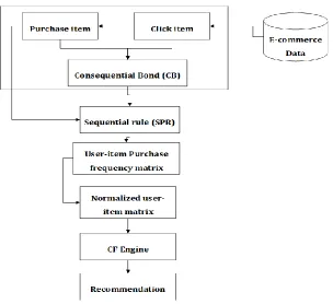
3.3 Architecture of Proposed System ... - 70 -

3.4 Example of HPCRec VS HSPRec system ... - 71 -

3.4.1 Xiao & Ezeife, 2018 (HPCRec18) ... - 72 -

3.4.2 Example of purposed HSPRec ... - 74 -

CHAPTER 4: EXPERIMENTAL EVALUATION AND ANALYSIS ... 79

-4.1 Historical Purchase Dataset Selection ... - 79 -

4.2 Dataset Evaluations ... - 79 -

4.2.1 Evaluation parameters ... - 80 -

4.2.2 Result evaluation and analysis ... - 82 -

4.2.3 Accuracy evaluation using precision ... - 83 -

4.3 Complexity Analysis ... - 84 -

4.3.1 Time complexity analysis of HSPRec algorithm ... - 84 -

4.4 Implementation and Coding ... - 85 -

CHAPTER 5: CONCLUSION AND FUTURE WORK ... 86

REFERENCES ... 87

-x

LIST OF TABLES

Table 1.1: E-commerce historical data ... - 3 -

Table 1.2: Daily sequential database created from historical purchase ... - 3 -

Table 1.3: Sequence database representing customer purchase ... - 4 -

Table 1.4: Candidate set (C2) generated from L1 GSP join L1 ... - 4 -

Table 1.5: 2-frequent sequences ... - 5 -

Table 1.6: Example to demonstrate merging of two sequences in GSP ... - 5 -

Table 1.7: n-frequent sequences generated by GSP algorithm ... - 5 -

Table 1.8: E-commerce historical data ... - 6 -

Table 1.9: Clickstream E-commerce data ... - 7 -

Table 1.10: User-item matrix for illustration of user based collaborative filtering ... - 8 -

Table 1.11: Input data to clustering algorithm ... - 14 -

Table 1.12: Maximum and minimum cluster centroids ... - 14 -

Table 1.13: Table showing computation of Euclidean distance ... - 14 -

Table 1.14: Table showing update of centroid in new cluster in K-means method ... - 14 -

Table 1.15: Cluster created by K-means method ... - 15 -

Table 1.16: Dataset to be classified by the decision tree ... - 15 -

Table 1.17: Transactional data to mine by Apriori algorithm ... - 17 -

Table 1.18: User-item rating matrix... - 18 -

Table 1.19: User-item purchased matrix generated from rating information ... - 18 -

Table 1.20: Normalized user-item frequency matrix created by Xiao & Ezeife, 2018 ... - 21 -

Table 1.21: E-commerce data containing consequential bond of click and purchase ... - 21 -

Table 1.22: Table showing existing E-commerce recommendations ... - 23 -

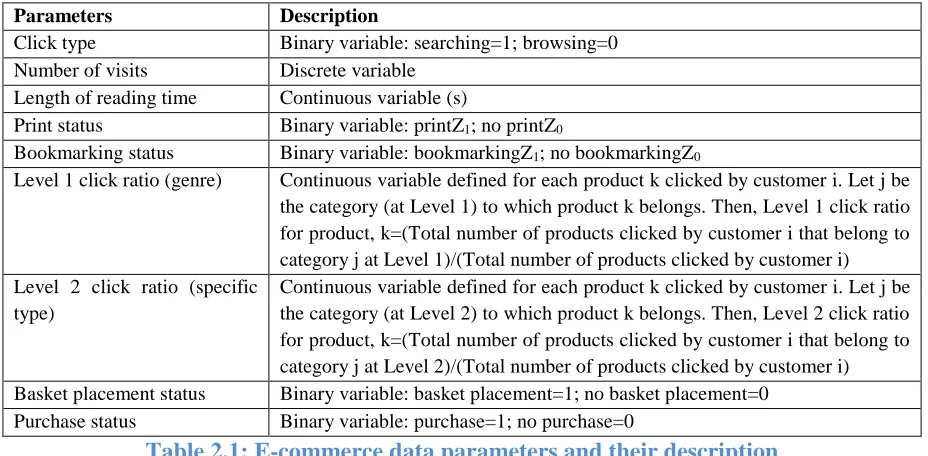
Table 2.1: E-commerce data parameters and their description ... - 27 -

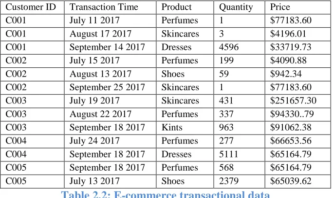
Table 2.2: E-commerce transactional data ... - 29 -

Table 2.3: E-commerce data clustering using RFM value ... - 30 -

Table 2.4: transaction clustering of E-commerce data ... - 30 -

Table 2.5: Transaction sequence clustering ... - 30 -

Table 2.6: Customer transaction cluster... - 31 -

Table 2.7: Association rules created from customer transaction cluster ... - 31 -

Table 2.8: Pseudo rating matrix ... - 32 -

Table 2.9:Pseudo rating matrix with temporal information ... - 33 -

Table 2.10: Pseudo rating matrix with rating function w(pi,lj) ... - 33 -

Table 2.11: Predefined rating function w ... - 33 -

Table 2.12: User-item rating matrix constructed from pseudo rating matrix ... - 33 -

Table 2.13: E-commerce clickstream data ... - 34 -

Table 2.14: User-item rating matrix for Niu, Chen, & Zhang, 2011 recommendation system - 36 - Table 2.15: Mean centering user-item rating matrix ... - 36 -

Table 2.16: Item-item similarity of mean centered rating matrix 2.16 ... - 37 -

xi

Table 2.18: Prediction rating matrix ... - 38 -

Table 2.19: Sequence database created by using rating value in descending order ... - 38 -

Table 2.20: n-frequent sequence for Li, Niu, Chen, & Zhang, 2011 recommendation ... - 38 -

Table 2.21: Choi, Keunho, Yoo, Kim, & Suh, 2012 historical user-item matrix ... - 39 -

Table 2.22: Implicit rating derived from user’s transactions ... - 40 -

Table 2.23: possible list of 2-items generated from frequent purchase (L1) ... - 41 -

Table 2.24: Frequent 2-item generated from candidate set (C2) ... - 41 -

Table 2.25: Table showing integration of CFPP and SPAPP ... - 42 -

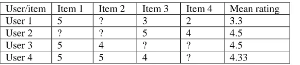
Table 2.26: User-item rating matrix for Zhao, Niu & Chen, 2013 recommendation system ... - 43 -

Table 2.27: User-item matrix showing mean rating of users on items ... - 43 -

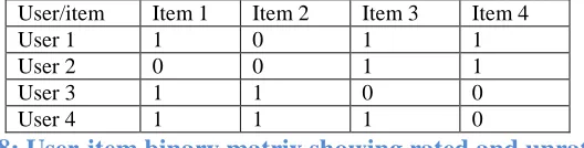
Table 2.28: User-item binary matrix showing rated and unrated items ... - 44 -

Table 2.29: Normalized user-item rating matrix... - 44 -

Table 2.30: Table showing item-item similarity ... - 44 -

Table 2.31: User-category frequency matrix ... - 46 -

Table 2.32: User spend time on category ... - 47 -

Table 2.33: User-category relative duration matrix ... - 47 -

Table 2.34: Users browsing path ... - 48 -

Table 2.35: Consequential table on left and purchase frequency table on right ... - 49 -

Table 2.36: Non-normalized user-item matrix on left and normalized matrix on right ... - 49 -

Table 2.37: Weighted transactional table of purchase set created from consequential bond ... - 50 -

Table 2.38: Weighted frequent transaction table ... - 50 -

Table 2.39: Support for item present in weighted frequent transaction table ... - 50 -

Table 2.40: Weight for item present in purchase pattern ... - 50 -

Table 2.41: Sequence Database representing customer purchase ... - 51 -

Table 2.42: Candidate set (C2) generated from L1 GSP join L1 ... - 52 -

Table 2.43: n-frequent sequences generated by GSP from sequence database ... - 52 -

Table 2.44: Sequence input database for prefixSpan ... - 53 -

Table 2.45: support for singleton sequences ... - 53 -

Table 2.46: Project database of sequence database ... - 54 -

Table 2.47: Projected database of sequence <(D)> ... - 54 -

Table 2.48: Frequencies of item presented in projected database of sequence <(D)> ... - 54 -

Table 2.49: project database of sequence <(D), (B)> and <(D), (C)> ... - 55 -

Table 2.50: Frequencies of item present in projected database of sequence <(D), (C)> ... - 55 -

Table 2.51: Projected database of sequence <(D), (C), (B)> ... - 55 -

Table 2.52: Input sequential database for SPADE... - 56 -

Table 2.53: Vertical data format of sequence database ... - 56 -

Table 2.54: Frequent 1-sequence with event ID and item ID ... - 56 -

Table 2.55: Process of generating 2-frequent sequences in SPADE ... - 57 -

Table 2.56: n-frequent sequences generated by SPADE algorithms ... - 57 -

xii

Table 3.2: Daily purchase sequential database ... - 60 -

Table 3.3: Enhanced user-item purchase frequency matrix ... - 61 -

Table 3.4: Consequential bond of sequence of click and purchase ... - 61 -

Table 3.5: Click sequential database ... - 62 -

Table 3.6: Weighted purchase patterns ... - 62 -

Table 3.7: Quantitatively rich user-item purchase frequency matrix ... - 62 -

Table 3.8: Normalized enrich user-item purchase frequency matrix ... - 63 -

Table 3.9: Historical E-commerce purchase data ... - 64 -

Table 3.10:Sequential database created from historical transactional data ... - 65 -

Table 3.11: Alternative representation of daily purchase sequential database ... - 65 -

Table 3.12: Weighted purchase pattern ... - 68 -

Table 3.13: Historical Click data ... - 71 -

Table 3.14: Historical purchase data ... - 71 -

Table 3.15: Consequential table from click and purchase historical data ... - 71 -

Table 3.16: User-item frequency matrix from purchase historical data ... - 72 -

Table 3.17: Normalized user-item frequency matrix ... - 72 -

Table 3.18: Weighted transactional table... - 73 -

Table 3.19: Quantitatively rich normalized user-item frequency matrix ... - 73 -

Table 3.20: User-item frequency matrix created from historical purchase ... - 74 -

Table 3.21: Daily purchase sequential database created from historical transaction data ... - 74 -

Table 3.22: Sequential rule created from n-frequent sequences ... - 74 -

Table 3.23: Rich user-item frequency matrix created with help of sequential rule ... - 75 -

Table 3.24: Sequential database created from consequential table ... - 75 -

Table 3.25: Sequential rule created from n-frequent sequences ... - 76 -

Table 3.26: Recommend item for click when purchase is not happened ... - 76 -

Table 3.27: CPS similarity using click and purchase ... - 77 -

Table 3.28: Weighted purchase patterns ... - 77 -

Table 3.29: Support for item present in weighted purchase patterns ... - 77 -

Table 3.30: Rich user-item purchase frequency matrix ... - 78 -

Table 3.31: Quantitatively rich purchase user-item purchase frequency matrix ... - 78 -

Table 4.1: Actual rating and predicted rating user-item matrix ... - 80 -

Table 4.2: Confusion matrix for recommendation system... - 80 -

xiii

LIST OF FIGURES

Figure 1.1: Decision tree for classification ... - 16 -

Figure 1.2: Improved user-item matrix on the right and traditional matrix on the left ... - 19 -

Figure 1.3: Historical sequential recommendation (HSPRec) ... - 24 -

Figure 2.1: Decision tree to show click and basket placement probability ... - 28 -

Figure 2.2: a) conventional recommendation system and b) Kim recommendation system .... - 28 -

Figure 3.1: Architecture of HSPRec showing modules and flow ... - 70 -

Figure 4.1: Historical purchase data (Amazon data) ... - 79 -

Figure 4.2: Function to compute mean absolute error (MAE)... - 80 -

Figure 4.3: Function to compute precision ... - 81 -

xiv

LIST OF EQUATIONS

Equation 1.1: Formula to Compute Cosine similarity ... - 9 -

Equation 1.2: Formula to compute Pearson Correlation coefficient ... - 9 -

Equation 1.3: Equation to compute mean rating ... - 10 -

Equation 1.4: Euclidean distance formula ... - 13 -

Equation 1.5: Equation to compute support of itemset i ... - 17 -

Equation 1.6: Equation to compute confidence of itemset i ... - 17 -

Equation 2.1: Association rule to mine customer behavior in LiuRec09 ... - 31 -

Equation 2.2: Formula to match target user purchase in LiuRec09 ... - 32 -

Equation 2.3: Equation to count support... - 34 -

Equation 2.4: Equation to compute lift value ... - 35 -

Equation 2.5: Pearson Correlation coefficient to compute similarity ... - 37 -

Equation 2.6: Equation to compute predicted rating in item-item similarity ... - 37 -

Equation 2.7: CF-based predicted preference ... - 40 -

Equation 2.8: Formula to compute hits of user on item and category ... - 45 -

Equation 2.9: Formula to compute frequency of hit ... - 45 -

Equation 2.10: Cosine similarity function to compute frequency similarity ... - 46 -

Equation 2.11: Formula to compute relative duration ... - 46 -

Equation 2.12: Cosine similarity function to compute duration similarity ... - 47 -

Equation 2.13: Equation to compute path similarity ... - 48 -

Equation 2.14: Equation to compute the total similarity ... - 48 -

Equation 2.15: Unit vector formula to normalize purchase frequency ... - 49 -

Equation 2.16: Longest common subsequence rate ... - 49 -

Equation 2.17: Longest common sequence (LCS) ... - 50 -

Equation 3.1: Sequential Pattern Rule generated from n-frequent sequences ... - 66 -

Equation 3.2: Sequence similarity function ... - 67 -

Equation 3.3: Cosine similarity function ... - 67 -

Equation 3.4: Formula to compute weight in WFPPM ... - 68 -

- 1 -

CHAPTER 1:INTRODUCTION

Recommendation systems provide a suggestion of items to the user in various decision-making processes such as what item to buy, what movies to watch, what music to listen to what online news to read (Ricci, Rokach, & Shapira, 2011). The main goal of the recommendation system is to generate meaningful recommendations to a user for items that might interest them. One of the important applications of recommendation systems is in the e-commerce domain. Recommendation system in e-commerce helps to model the business process through analysis of customer requirements or their purchase behaviors (Schafer, Frankowski, Herlocker, & Sen, 2007). Recommendation systems use data mining technologies such as classification, clustering, association rule mining, frequent pattern mining, and sequential pattern mining to generate a meaningful representation of user purchase data (Han, Pei, & Kamber, 2011).

Traditionally, collaborative filtering was one of the most widely used recommendation technique, and it depends on explicit rating of items provided by users, but many users may not be ready to provide the items ratings. To resolve the rating problem, some implicit rating techniques (Choi, Keunho, Yoo, Kim, & Suh, 2012) derived from user behaviors (for example, purchases, clicks) across E-commerce and clickstream data analysis techniques (Kim, Yum, Song, & Kim, 2005), (Liu, Lai, &Lee,2009) are used. However, users purchase behaviors are always dynamic in nature and purchase of items may be different in each purchase. So, one of the main challenges in the field of recommendation system is to integrate sequential patterns of purchases with collaborative filtering because collaborative filtering finds closest neighbors between users or items without considering i) sequential purchase patterns ii) click and purchase behaviors iii) possible reasons for changes in user purchase habits. Various recommendation techniques such as collaborative filtering, content-based, and hybrid collaborative filtering approaches have been developed. While

Collaborative filtering (CF) does not take into account the properties of the items but uses only the

preference (rating or voting) provided by users for items, the content-based approach makes

- 2 -

recommendation and can serve to solve the cold start problem when there is no rating information for by a user on an item. However, such approaches suffer from a major drawback because they are not able to capture the E-commerce domain with sequential information of customer purchase behavior. Furthermore, sequential data may be available in a historical form, clickstream form. So, one of the main challenges in E-commerce recommendation is to generate the best recommendation suggestions from historical or clickstream sequential data to capture customer shopping behavior with respect to time.

1.1 Sequential Pattern

Sequential patterns are ordered set of items (events) that are occurring with respect to time (Agrawal & Srikant, 1996). A sequential pattern is denoted in the angular bracket (< >), and each itemset contains sets of items, where each item enclosed in parenthesis ( ) separated by commas represents a set of items purchased at the same time. For example, E-commerce sequential pattern < (Bread, Milk), (Bread, Milk, Sugar), (Milk), (Tea, Sugar)> means customer bought Bread and Milk together on first purchase, then bought Bread, Milk, and Sugar together on second purchase, then bought Milk on third purchase, and finally, bought Tea and Sugar together on fourth purchase. A sequential pattern with n-itemsets is called an n-events sequence. For example, if we consider only 2-itemsets, then we will have 2-events sequence such as <(Bread), (Milk)> or < (Bread), (Tea, Milk)>. Additionally, an item can occur at most once in an event (itemset) but can occur multiple times in different events (itemsets) within the same sequential pattern. Thus, the number of instances of items in a sequence is called the length of a sequence. For example, < (Bread, Milk), (Bread, Milk, Sugar), (Milk), (Tea, Sugar)> is 4-events sequence with length 8.

1.2 Sequential database

Sequence database is composed of a collection of sequences {s1, s2,…,sn} that are arranged with

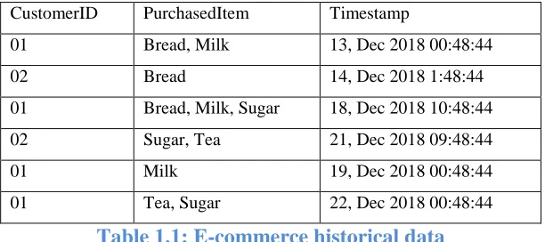
respect to time (Han, Pei & Kamber, 2011). A sequence database can be represented as a tuple <SID, sequence-item sets>, where SID: represents the sequence identifier and sequence-item sets specifies the sets in item enclosed in parenthesis ( ). For example, let us consider an example of E-commerce historical daily purchase data of grocery store as shown in Table 1.1, which contains CustomerID to represents a customer, PurchasedItem to represents a set of purchase items by customers and Timestamp to represents a time when purchased occurred.

- 3 -

CustomerID PurchasedItem Timestamp

01 Bread, Milk 13, Dec 2018 00:48:44

02 Bread 14, Dec 2018 1:48:44

01 Bread, Milk, Sugar 18, Dec 2018 10:48:44 02 Sugar, Tea 21, Dec 2018 09:48:44

01 Milk 19, Dec 2018 00:48:44

01 Tea, Sugar 22, Dec 2018 00:48:44

Table 1.1: E-commerce historical data

The daily sequential database created from historical data (Table 1.1) is present in Table 1.2, where SID represents the sequence identity. As we can see in Table 1.2, SID(01) contains <(Bread, Milk),(Bread, Milk, Sugar),(Milk),(Tea, Sugar)>, which means customer (01) first purchased Bread and Milk together then purchased Bread, Milk and Sugar together in second purchase and Milk in third purchase. Finally, Tea and Sugar together at last purchase.

SID Sequences

01 <(Bread, Milk),(Bread, Milk, Sugar),(Milk),(Tea, Sugar)> 02 <(Bread),(Sugar, Tea)>

Table 1.2: Daily sequential database created from historical purchase

1.3 Sequential Pattern Mining

Sequential pattern mining algorithm (for example, Generalized Sequential Pattern (GSP) (Agrawal & Srikant, 1996)) discover repeating patterns (known as frequent sequences) from input E-commerce historical sequential database that can be used later to analyze the user purchase behavior by finding the association between items. In other words, it is a process of extracting sequential patterns whose support exceeds a predefined minimum support threshold. Formally, Given (i) a set of sequential records (called sequences) representing a sequential database D, (ii) a minimum support threshold (iii) a set of k unique items or events I = {i1, i2, . . . , ik}, the problem

of mining sequential patterns is of finding the set of all frequent sequences S in the given sequence database D of items I at the given minimum support. The details of different types of sequential pattern mining algorithms are present in section 2.2.

Example of sequential pattern mining using GSP algorithm

- 4 -

meeting the Apriori property. The Apriori property is used to prune candidate sequential patterns whose subsets are not already frequent in earlier rounds as these patterns cannot be frequent and

there is no need to scan the database for their support count. The GSP algorithm then generates candidate (k+1)-sequences from (Fk) sequences as Fk GSP-join Fk. The algorithm iterates between

the candidate generate and prune step, and support count step until either a Cm or an Fn step

generates an empty set. Details about the GSP-join operation are illustrated further through an example. Let us, consider daily sequential database (Table 1.3) as input, minimum support=2 and candidate set (C1) = {A, B, C, D, E, F, G}.

SID Sequences

1 <(A),(B),(FG),(C),(D)> 2 <(B),(G),(D)>

3 <(B),(F),(G),(A,B)> 4 <(F),(A,B),(C),(D)> 5 <(A),(B,C),(G),(F),(D,E)>

Table 1.3: Sequence database representing customer purchase

Step 1: Find 1- frequent sequence (L1) to keep only sequence with occurrence or support count in

the database greater than or equal to minimum support. For example, L1= {<(A):4>, <(B):5>,

<(C):3>, <(D):4>, <(F):4>, <(G):4>}.

Step 2: Generate candidate sequence (Ck=2) using L1 𝐺𝑆𝑃𝑗𝑜𝑖𝑛 L1

To generate larger candidate set 2, use 1-frequent sequences found in step 1, which can be written as L (k-1) 𝐺𝑆𝑃𝑗𝑜𝑖𝑛 L (k-1) and it requires every sequence (W1) found in first L (k-1) joins with other

sequence (W2) in the second, if subsequences obtained by removal of first element of W1 and last

element of W2 are same. In our case, the possible 2-length candidate (Ck=2) sets generated using 𝐺𝑆𝑃𝑗𝑜𝑖𝑛 are present in Table 1.4.

<(A),(A)> <(A),(B)> <(A),(C)> <(A),(D)> <(A),(F)> <(A),(G)>

<(B),(A)> <(B),(B)> <(B),(C)> <(B),(D)> <(B),(F)> <(B),(G)>

<(C),(A)> <(C),(B)> < (C),( C)> <(C ),(D)> <( C),(F)> <( C),(G)>

<(D),(A)> <(D),(B)> <(D),(C)> <(D),(D)> <(D),(F)> <(D),(G)>

<(F),(A)> <(F),(B)> <(F),(C)> <(F), (D)> <(F),(F)> <(F),(G)>

<(G),(A)> <(G),(B)> <(G),(C)> <(G),(D)> <(G),(F)> <(G),(G)>

<(A,B)> <(A,C)> <(A,D)> <(A,F)> <(A,G)> <(B,C)>

<(B,D)> <(B,F)> <(B,G)> <(C,D)> <(C,F)> <(C,G)>

<(D,F)> <(D,G)> <(F,G)>

- 5 -

Step 3: Find 2- frequent sequences (L2) by counting occurrence of 2-sequences in candidate

sequence (C2) to keep only sequence with occurrence or support count in the database greater than

or equal to minimum support. For example,

L2=

Table 1.5: 2-frequent sequences

Step 4: Generate candidate sequence (Ck=3) using L2 𝐺𝑆𝑃𝑗𝑜𝑖𝑛 L2

Use same candidate generation technique used in Step 2. An example of two sequences merged is present in Table 1.6.

W1 Sequence W2 Sequence Merged Sequence <(A),(B)> <(B),(C)> <(A), (B), (C)> <(A), (B,C)> <(B,C), (D)> <(A), (B,C), (D)>

Table 1.6: Example to demonstrate merging of two sequences in GSP

Step 5: Find 3- frequent sequences (L3) to keep sequences with occurrence or support count in the

database greater than or equal to minimum support. For example, L3= {< (F), (C), (D)>, < (B), (G), (D)>, < (B), (F), (D)>, < (B), (C), (D)>, < (A), (G), (D)>, < (A), (F), (D)>, < (A), (C), (D)>}.

Step 6: Repeat process of candidate generation and pruning until result of candidate generate (Ck)

and prune (Lk) for finding frequent sequence is an empty set.

Output: Finally, the output frequent sequences are union of L1 U L2 U L3 U L4

1-Frequent Sequences

2-Frequent Sequences 3-Frequent Sequences 4-Frequent Sequences

<(A)>, <(B)>, <(C)>, <(D)>, <(F)>, <(G)>

<(A), (B)>, < (A, B)>, <(A), (C)>, <(A), (D)>, <(A), (F)>, <(A), (G)>, <(B), (C)>, <(B), (D)>, <(B), (F)>, <(B), (G)>, <(C), (D)>, <(F), (A)>, <(F), (B)>, <(F), (C)>, <(F), (D)>, <(G), (D)>

<(F), (C), (D)> <(B), (G), (D)> <(B), (F), (D)> <(B), (C), (D)> <(A), (G), (D)> <(A), (F), (D)> <(A), (C), (D)> <(A), (B), (G)> <(A), (B), (F)> <(A), (B), (D)>

<(A), (B), (G), (D)> <(A), (B), (F), (D)>

Table 1.7: n-frequent sequences generated by GSP algorithm <(A), (B)> <(A, B)> <(A), (C)> <(A), (D)> <(A), (F)> <(A), (G)>

<(B), (C)> <(B), (D)> <(B), (F)> <(B), (G)> <(C), (D)> <(F), (A)>

- 6 -

1.4 E-commerce Data Types

1.4.1 E-commerce historical data

E-commerce historical data consists of a list of items clicked and/or purchased by a user over a specific period of time. A fragment of E-commerce historical database data is present in Table

1.8 with schema {Uid, Click, Clickstart, Clickend, Purchase, Purchasetime}, where Uid represents User identity, Click represents a set of items clicked by a user, Clickstart and Clickend represent the timestamp when user started clicking item and when click is terminated. Furthermore, Purchase contains a set of items purchased by a user and Purchasetime represents timestamp when purchase happened.

Table 1.8: E-commerce historical data

1.4.2 E-commerce clickstream data

Clickstream data represents the visitors’ paths through E-commerce sites. A series of E-commerce pages visited by a user in a single visit is referred to as a session. Clickstream data in an E-commerce environment is a collection of sessions. Clickstream data can be derived from raw page requests (referred to as hits) and their associated information (such as timestamp, IP address, URL, status, number of transferred bytes, referrer, user agent, and, sometimes, cookie data) recorded in Web server log files (Bucklin & Sismeiro, 2009). Analysis of clickstreams shows how an E-commerce site is navigated and used by E-E-commerce users. In an E-E-commerce environment, clickstreams in online stores provide information essential to understanding the effectiveness of marketing and merchandising efforts, such as how customers find the store, what products they see, and what products they buy. Analyzing such information embedded in clickstream data is critical to improve the effectiveness of recommendation in online stores. An example of E-commerce Clickstream data is present in Table 1.9.

Uid Click Clickstart Clickend Purchase Purchasetime

1 1,2,3 2014-04-04 11:25:14 2014-04-04 11:45:19 1, 2 2014-04-04 11:30:11

1 7,5,3 2014-04-05 15:30:07 2014-04-05 15:59:36 3 2014-04-05 15:56:32

2 1, 4 2014-04-13 4:01:11 2014-04-13 4:30:15 1, 4 2014-04-13 04:04:34

2 1, 2,5, 6 2014-04-17 11:30:18 2014-04-17 11:50:19 1, 2,5, 6 2014-04-17 11:44:55

3 5 2014-04-23 11:00:05 2014-04-23 11:20:15 5 2014-04-23 11:06:37

4 6,6,7 2014-04-26 9:45:11 2014-04-26 10:20:13 6, 7 2014-04-26 10:06:37

- 7 -

Session ID Timestamp ItemID CategoryID

*****Ef4d7 2018-08-24T22:38:13+00:00 2145456502 3

*****Ef4d7 2018-08-24T20:38:12+00:00 21453650011 4 *****Ef4d7 2018-08-24T23:38:10+00:00 214536503 1 *****KM5M7 2018-08-24T22:38:14+01:00 2145775612 2 *****KM5M7 2018-08-24T22:38:14+03:03 2146627421 4 *****KM5M7 2018-08-24T22:38:14+04:05 214662742 6 *****KM5M7 2018-08-24T22:38:14+05:07 214825110 3

Table 1.9: Clickstream E-commerce data

The clickstream data given in Table 1.9, consists of session ID (*****Ef4d7, *****KM5M7) which represents user identity, timestamp (2018-08-24T23:38:10+00:00) represents the time when item visited, ItemID (2146627421, 214662742) represents the item visited by the user and CategoryID represents a category (e.g., milk belongs to dairy category) where items belong.

1.5 Consequential Bond (CB)

E-commerce data contains information’s of clicks and purchases referred to as a consequential bond, and it is introduced by Xiao and Ezeife, 2018 in their HPCRec18 system. The term consequential bond is originated from the concept that customer who will click some items will ultimately purchase an item from a list of clicks in most of the cases. For example, historical data present in Table 1.8 shows that user 1 clicked items {1, 2, 3} and ultimately purchased {1, 2}; thus, there is a relationship between click and purchase.

1.6 Types of E-commerce Recommendation Systems

Based on how recommendations are made, recommender systems are usually classified into three categories:

- 8 -

disadvantage of this technique is the need to have in-depth knowledge and description of the features of the items in the profile.

2. Collaborative filtering (CF): Collaborative filtering (CF) does not take into account the properties of the items but only the preference (rating or voting) provided by users for items

(Aggarwal & Charu, 2016). Thus, CF predicts rating of items using either a user-based or

item-based approach. The user-based CF is based on the similarity between users, and items

and item-based CF is based on the similarity between items and items. The similarity is

computed by using one of the similarity measures such as (Cosine similarity, Pearson

Correlation Coefficient and Jacquard similarity) then these similarity values are used to predict

the unknown ratings of a user on an item using Top-N neighbors. The major problems of CF

are cold start, sparsity, and scalability.

3. Hybrid filtering: Both CF and CBF have their benefits and demerits; therefore, if we combine both of them together, then the benefits of both can be used to overcome the demerits of others

(Kumar & Fan, 2015). For example, CF provides recommendations using rating matrix now

what happens when there is no rating given by a user (new user) then in such case the contents

of user-item (CBF filtering) can be used with CF for recommendations.

1.7 Collaborative Filtering in E-commerce

Collaborative filtering makes a recommendation to a target customer based on the purchase behavior of customers whose preference is similar to a target customer. It is one of the widely used recommendation technique. Given a user-item rating matrix-R (such as Table 1.10),

Item 1 Item 2 Item 3 Item 4 Item 5 Item 6 Mean rating

User A 7 6 7 4 5 4 33/6

User B 6 7 ? 4 3 4 24/5

User C ? 3 3 1 1 ? 8/4

User D 1 2 2 3 3 4 15/6

User E 1 ? 1 2 3 3 10/5

Table 1.10: User-item matrix for illustration of user based collaborative filtering

where a value of matrix is a rating 𝑟𝑢𝑗𝑖𝑘, where uj represents user j as in {u1, u2, . . . , uj} and ik represents item k as in { i1, i2, . . . , ik}. Furthermore, the rating can be either an explicit rating or an implicit rating. Goal of collaborative filtering is to predict unknown rating 𝑟𝑢𝑖 of useru on itemi

- 9 -

1. Compute the mean rating for all user uj using all of their rated items.

2. Calculate the similarity between the target user (v) and all other users uj. Similarity can be

computed with Cosine Similarity (v,uj) or Pearson Correlation Coefficient function.

3. Find similar users of the target user (v) as Top-N users’.

4. Predict rating for the target user (v) for item i using only rating of v’s Top-N peer group. There are two types of collaborative filtering, user based and item based collaborative filtering. User-based collaborative filtering takes the ratings from similar users of the target user whereas item-based collaborative filtering considers the ratings from similar items of the target item.

1.7.1 User- based collaborative filtering

User-based collaborative filtering uses ratings of similar users for making a recommendation to a target user. The necessary algorithm of user-based collaborative filtering along with a running example is given below:

Input: user-item rating matrix R, containing 𝑟_{𝑢𝑗𝑖𝑘}, whereuj represents user j as in {u1, u2, . . . , uj}

and ik represents item k as in { i1, i2, . . . , ik}.

Output: Predicted ratings for previously unknown rating.

Major steps of collaborative filtering using user-based neighborhood method (Aggarwal & Charu, 2016) are:

1. Compute the mean rating for all user uj using all of their rated items.

2. Calculate the similarity between the target user (v) and all other users uj. Similarity can

be computed by Cosine Similarity or Pearson Correlation coefficient function as given in

Equation 1.1 and Equation 1.2.

Cosine (u, v)= 𝑢⃗⃗ . 𝑉⃗⃗⃗

||𝑢||.||𝑣||

=

𝑟_𝑢1 ⋅ 𝑟_𝑣1 + 𝑟_𝑢2 ⋅ 𝑟_𝑣2+ … +𝑟_𝑢𝑛 ⋅ 𝑟_𝑣𝑛 √𝑟_𝑢12+𝑟_𝑢22+⋯+𝑟_𝑢𝑛2 ∗ √𝑟_𝑣12+𝑟_𝑣22+⋯+𝑟_𝑣𝑛2

Equation 1.1: Formula to Compute Cosine similarity

In Equation 1.1, 𝑟_𝑢1 represents rating of user u on item 1, and 𝑟_𝑣1 represents rating of user v on item 1 respectively.

Pearson Correlation (u, v)= ∑i∈I(rui−r⃗⃗⃗⃗ u)∗(rvi−r⃗⃗⃗⃗ v)

√∑i∈I(rui−r⃗⃗⃗⃗ u)2∗ √∑i∈I(rvi−r⃗⃗⃗⃗ v)2

Equation 1.2: Formula to compute Pearson Correlation coefficient

- 10 -

Mean rating (𝑟⃗⃗⃗⃗⃗ =_𝑢) ∑𝑖∈𝐼𝑟𝑢𝑖

|𝑁𝑢𝑚𝑏𝑒𝑟 𝑜𝑓 𝑖𝑡𝑒𝑚𝑠|

Equation 1.3: Equation to compute mean rating

3. Find similar users of the target user (v) as Top-N users’.

4. Predict rating of target user (v) for item i using only ratings of v’s Top-N peer group. Example of user based collaborative filtering

Let us consider user-item rating matrix (Table 1.10) as input and our goal is to predict a rating of User C on Item 1 using collaborative filtering.

Step 1: Compute the mean rating for User A, User B, User C, User D, and User E using all of their rated items

For, User1= 33/6=5.5, User 2=24/5=4.8, User 3=8/4=2, User 4=15/6=2.5 and User 5=10/5=2 Step 2: Compute similarity between User C and others users

The similarity between User C and all others users can be computed using Cosine similarity or Pearson-Correlation Coefficient. In our case, we have used Cosine similarity, which is present in

Equation 1.1. For example, SIM (User A, User C) = 6∗3+7∗3+4∗1+5∗1

√62₊₇2₊₄2₊₅2_∗√32₊₃₊₁2₊₁2 = 0.956. Similarly, SIM (User B, User C) =0.981, SIM (User D, User C) =0.789 and SIM (User E, User C) =0.645. Step 3: Select the Top-N (in our case N=2) neighbor of User C by comparing similarity

Select Top-N neighbor of User C by comparing Cosine similarity. In our case, User A and User B have the highest similarity with User C. So, they are selected as Top-N neighbors.

Step 4: Compute the raw rating value using Top-N users (User A and User B)

To compute raw rating, Top-N users rating on item are used. For example, Raw ratingUser-C, item1 is

calculated by using rating for of User A on Item 1 and rating of User B on Item 1. Raw rating User-C, item 1 = 7 ∗ 0.956+ 6 ∗ 0.981

0.956 + 0.981 = 6.49

Raw rating User-C, item 6= 4 ∗ 0.956+ 4∗ 0.981

0.956 + 0.981 = 4

Step 5: Compute mean centric rating

- 11 -

computed by subtracting rating of User A on Item 1 and mean rating of User A (in our case, 7-5.5=1.5).

Mean centric rating User-C, item 1=2+ 1.5 ∗ 0.956 + 1.2 ∗ 0.981

0.956 + 0.981 = 3.35

Mean centric rating User-C, item 6= 0.86

There are some fundamental issues with collaborative filtering; they are:

(1) Cold start: When new items or new users appear in the database, these items may not be rated by any users; thus, preferences of users' may be unknown.

(2) Sparsity issue: When known rating data takes only a very small proportion in the user-item rating matrix, for instance, the amount of products is usually billions in the real world and most of the users only purchased probably hundreds of them, which leads to confusing and compromised recommendations. To address the sparsity issues, in this thesis, we have used sequential patterns of click and/or purchase to derive a rule to provide the relationship between already clicks or purchased items and recommended items to fill the missing rating for an item to improve the item matrix quantitatively (providing possible value for the unrated item or 0 value item in user-item matrix).

(3) Scalability issue: As the numbers of users and products grow rapidly, the time complexity and space complexity issues become more prominent.

1.8 Goal of E-commerce Recommender System

1) Converting browser to buyer: In an E-commerce environment, large amounts of information

are available, so it can be hard for a user to find the product they are looking for. Thus, recommender systems help consumers to find products they intend to buy (Schafer, Konstan, & Riedl, 2010).

2) Increasing cross-sell products: Recommender systems can improve the cross-sales product ratio by suggesting additional products. In general, a recommender system suggests products based on the customer’s cart and purchase history.

- 12 -

1.9 Need of Sequential Purchase Data in E-commerce Recommendation

1) User purchase habit changes with time: Collaborative filtering (CF) methods make a recommendation to a target customer based on the purchase behavior of other customers whose preferences are similar to those of the target customer. Thus, CF cannot capture the changes in purchase behavior of the customer over time, and integrating sequential rule in E-commerce can capture the customer purchase behavior over time.

2) Integrating frequency, price factor in recommendation: Traditional collaborative filtering technique, only consider the rating of an item for making a recommendation. Only considering the rating factor cannot provide a good recommendation to users because user choice may depend on product quantity, price and overall profit gained from purchased.

3) Taking care of timing factor during E-commerce recommendation generation: In E-commerce, some users may purchase items regularly, while other users may purchase items irregularly. So, recommendation generation by considering irregular users may provide a wrong recommendation to regular users.

1.10 Data Mining

- 13 -

data warehouse and to be understandable and usable by marketing professionals, while classic statistical tools cannot fulfill these objectives.

1.10.1 Clustering

Clustering is a process of grouping a set of related objects in such a way that objects in the same group are similar to each other (Jain & Dubes, 1998). It is an unsupervised data mining technique that can automatically divide the data into a set of clusters or groups of similar items. The K-means clustering (Hartigan & Wong, 1979) is one of the widely accepted clustering approaches in the field of data mining (Steinbach, Karypis, & Kumar, 2000). K-means clustering is used, when we have data without defined categories or groups and goal of this algorithm is to find groups in

the data, with the number of groups represented by the variable K. The algorithm works iteratively

to assign each data point to one of K groups based on the features that are provided. The K-means clustering algorithm consists of four major steps:

1. Randomly pick centroid from available objects. Let us consider, we do have n objects {I1, I2, I3, …., In} and their attributes as {A1, A2,….An} then, we can consider (H1, W1)

as a centroid of objects considering height and weight as major attributes.

2. Calculate the distance between the centroid and other objects. The distance can be calculated using the Euclidean distance formula (Equation 1.4).

E. D=√(𝐀𝑯− 𝐇𝟏)𝟐 + (𝑨𝒘− 𝐖𝟏)𝟐

Equation 1.4: Euclidean distance formula

Where, XH= Observation value of height, H1= Centroid value of cluster 1 for height, Xw=

Observation value of height, W1= Centroid value of cluster 1 for weight

3. Update centroid of each new cluster, by computing the average attributes of all object in a cluster.

4. Repeat step 1, 2 and step 3 until the centroids stop changing. Example of K-means clustering

- 14 - Height Weight 185 72 170 56 168 60 179 68 182 72 188 77

Table 1.11: Input data to clustering algorithm

Step 1: Initialize cluster centroid

Let’s consider, two centroids one containing minimum value of Height, Weight and another containing maximum value of Height, Weight as given in Table 1.12.

Cluster Initial Centroid Height Weight

Cluster 1 185 72

Cluster 2 170 56

Table 1.12: Maximum and minimum cluster centroids

Step 2: Select objects value from input data and calculate Euclidean Distance from centroids Once centroids (maximum, minimum) are fixed, select input value from input data and calculate Euclidean distance using Equation 1.4. Here, we are using (Height: 168, Weight: 60) as object value from input data.

Euclidian Distance from Cluster 1 Euclidian Distance from Cluster 2 Chosen cluster √(168 − 185)2_{+ 60 − 72}2_{= 20.808 √(168 − 185)}2_{+ (60 − 72)}2 _{= 4.472 Cluster 2}

Table 1.13: Table showing computation of Euclidean distance

From Euclidean distance, we can see that record with (168, 60) is very close to cluster 2.

Step 3: Update centroid of each new cluster, by computing the average attributes of all objects in each cluster.

Cluster Updated

Centroid Height Weight

Cluster 1 185 72

Cluster 2 (170+168)/2=169 (56+60)/2=58

Table 1.14: Table showing update of centroid in new cluster in K-means method

- 15 -

Objects Cluster

{(185,72), (179,68), (182,72), (188,77)} Cluster 1 {(170,56), (168,60)} Cluster 2

Table 1.15: Cluster created by K-means method

1.10.2 Classification

Classification is used to classify an item in a set of predefined set of classes or groups. The paramount difference between classification and clustering is that classification is used in

supervised learning technique where predefined labels are assigned to instances by properties; on

the contrary, clustering is used in unsupervised learning, where similar instances are grouped,

based on their features or properties (Arabie, Phipps, & Soete, 1996). The classification process involves the training set and testing set. The training dataset is used to train model, by pairing the input with expected output. Then, the same classification model is applied to the test data having unknown target class values, to check for its prediction accuracy. The classification by decision tree induction (Apté, Chidanand, & Weiss, 1997) is one of the most widely used classification technique. The decision tree has two types of nodes, decision node (which are internal nodes) and leaf node. A decision node specifies test (asks a question) on a single attribute. A leaf node indicates a class. To use the decision tree in testing, the tree top-down according to attribute values with given test instance until a leaf node.

Example of classification by decision tree

Let us consider the example data set as given in Table 1.16 for classification and our main goal is to determine, whether a user is eligible for a credit card or not using the decision tree.

TID AGE JOB_STATUS HOUSE_STATUS CREDIT_SCORE Credit Offer

1 Young FALSE FALSE Fair No

2 Young FALSE FALSE Good No

3 Young TRUE TRUE Fair Yes

4 Middle TRUE TRUE Good Yes

5 Middle FALSE TRUE Excellent Yes

Table 1.16: Dataset to be classified by the decision tree

- 16 -

Figure 1.1: Decision tree for classification

In Figure 1.1, Age is the root node, which asks the question: what is the age of the applicant? It has three possible answers or outcomes, which are the three possible values of Age (Young, middle and old).

1.10.3 Association Rule

Association rules analysis is an unsupervised technique to discover how items are associated with each other (Ma & Liu, 1998). The association rule consists of two parts the lefthand side is called antecedent, and the righthand side is called consequent. Association rule is represented in the form X-> Y, where X and Y belong to a candidate set I= {i1, i2....in} of n items. Association rule is

performed in two stages i) finding all frequent patterns (itemsets) having support greater than or equal to minimum support ii) finding all rules from frequent patterns with confidence greater than or equal to minimum confidence. Association rule finds the relationship between the items in the rule. For example, Bread->Milk implies that if product Bread is bought customers also buy product Milk. The Apriori algorithm (Agrawal & Srikant, 1994) is a popular algorithm for association rule mining, and it works in two steps i) generate frequent itemsets ii) pruning the itemsets based on the user-defined support. Apriori algorithm takes a transactional database and output is frequent itemsets that satisfied minimum support. So, in the first step, support count of each item in the candidate set (C1) is calculated, and those items that don’t satisfy the minimum support are pruned

and produced frequent set (L1). In the next step, the candidate set (C2) is produced by Apriori join

method by L1 App-join L1. This process is iterative until can’t produce more candidate set. In

Association rule, confidence and support are two major factors, which can be computed by

- 17 -

Support of item i = (number of occurences of i)

(𝑛𝑢𝑚𝑏𝑒𝑟 𝑜𝑓 𝑑𝑎𝑡𝑎𝑏𝑎𝑠𝑒 𝑡𝑟𝑎𝑛𝑠𝑎𝑐𝑡𝑖𝑜𝑛𝑠)

Equation 1.5: Equation to compute support of itemset i

Confidence of item i = (number of occurences of i)

(𝑛𝑢𝑚𝑏𝑒𝑟 𝑜𝑓 𝑜𝑐𝑐𝑢𝑟𝑎𝑛𝑐𝑒𝑠 𝑜𝑓 𝑡ℎ𝑒 𝑎𝑛𝑡𝑒𝑐𝑒𝑑𝑒𝑛𝑡 𝑜𝑓 𝑡ℎ𝑒 𝑖𝑡𝑒𝑚 𝑖)

Equation 1.6: Equation to compute confidence of itemset i

Example of association rule

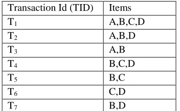
Let us consider transactional data as shown in Table 1.17 as input, where candidate set (C1) = {A,

B, C, D}, minimum support=3, and our goal is to find frequent items to create possible association rules.

Transaction Id (TID) Items

T1 A,B,C,D

T2 A,B,D

T3 A,B

T4 B,C,D

T5 B,C

T6 C,D

T7 B,D

Table 1.17: Transactional data to mine by Apriori algorithm

Step 1: Find frequent item (L1) from candidate set (C1)

The principal step in Apriori process is to find frequent item by the counting occurrence of each item. The items that don’t satisfy the minimum support count are pruned and produced frequent item (L1). In our case, frequent item (L1) = {A:3, B:6, C:4, D:5}.

Step 2: Generate candidate set (C2) from frequent item (L1) by Apriori join (L1 App-join L1)

We can generate a candidate set (C2) by L1 App-join L1. Frequent item (L1) can be joined only

with an item that comes after it in frequent item (L1). Which will give candidate set (C2) = {AB,

AC, AD, BC, BD, CD}.

Step 3: Find frequent item (L2) from candidate set (C2)

Frequent item (L2) is obtained by following the same procedure as in step 1. We can count the

occurrence of each item in candidate set (C2), and infrequent items are removed to create frequent

itemset (L2) = {AB: 3, BC: 3, BD: 4, CD: 3}.

Step 4: Generate candidate set (C3) from frequent item (L2) by Apriori join (L2 App-join L2)

We can apply the same process as in step 2 to generate candidate set (C3) by joining L2 with L2

- 18 - Step 5: Find frequent item (L3) from candidate set (C3)

None of the item in candidate set (C3) satisfied minimum support. So, we need to stop here and

join frequent item to get the final frequent item (L) =L1 U L2= {A, B, C, D, AB, BC, BD, CD}.

1.11 Existing E-commerce Recommendation Systems

There are different kinds of E-commerce data such as historical or clickstream. The historical data represents the list of an item purchased by the users over the time, which may consist of several attributes such as transactional ID, category ID, product ID, purchased Time, rating and many more. Many researchers tried to predict the users interest to items by using the rating of items provided by users (explicit rating - rate or vote of items within the specified range with available rating or voting system) as principle parameter (Sarwar, Karypis, Konstan & Riedl, 2001), (Herlocker, Konstan, Terveen & Riedl, 2004) in collaborative filtering. An example of explicit user-item rating matrix is present in Table 1.18.

User/Item Item1 Item2 Item3 Item4 Item5 Item6

User1 5 4 5 3 3 2

User2 4 3 ? 2 3 2

User3 ? 3 3 1 1 ?

User4 1 2 2 3 3 3

Table 1.18: User-item rating matrix

On another side, every user may not provide the rating for the purchased items or may not purchase items once they clicked or placed inside a basket. So, to alleviate this problem, researcher finds a way of representing user-item purchased by binary information (implicit rating- rating derived from user’s behaviors such as click, purchase), such as 1 for purchased/rated or 0 for non-purchased/unrated item. But, binary user-item matrix (Table 1.19) may be unable to provide information of click, basket placement, and purchase behavior.

User/Item Item1 Item2 Item3 Item4 Item5 Item6

User1 1 1 1 1 1 1

User2 1 1 0 1 1 1

User3 0 1 1 1 1 0

User4 1 1 1 1 1 1

Table 1.19: User-item purchased matrix generated from rating information

- 19 -

1) Probability based decision tree approach- KimRec05 (Kim, Yum, Song, & Kim, 2005): It used a binary user-item matrix to visualize the click and purchase behavior of a user and made a non-purchased item (0) more informative in the user-item matrix by computing the probability of purchase after basket placement. This approach is based on forming a decision tree from user’s behaviors such as searching, clicking to gives the proportion of users taking that path and its related probability. When new users arrive, it finds the right path based on basement placement probability. Finally, binary user-item rating matrix is filled with basket placement probability (as shown in Figure 1.2) to improve the user-item rating matrix before applying collaborative filtering. But KimRec05 is failed to provide: (a) Frequency of item purchased because a user may purchase the same item different number of times according to the time span (b) Unable to capture sequential purchase behavior (c) Fail to integrate E-commerce historical data.

1 1 0 0 0 5 4 0 1 3 0 0 1 2 1 0 1 1 4 3 2 1 Customer Customer Customer Customer Customer CD CD CD CD 1 1 44 . 0 15 . 0 82 . 0 5 4 15 . 0 1 3 44 . 0 62 . 0 1 2 1 15 . 0 1 1 4 3 2 1 Customer Customer Customer Customer Customer CD CD CD CD

(a) Conventional Recommender System (b) Proposed Recommender System

Figure 1.2: Improved user-item matrix on the right and traditional matrix on the left

- 20 -

user based on the frequency count of the item scanning the purchase data of k-neighbors. The major drawbacks of LiuRec09 are: (a) It does not learn sequential purchase during user-item matrix creation (b) Utility of an item such as frequency and price are ignored during the recommendation generation.

3) User transactions based preference approach- ChoiRec12 (Choi, Keunho, Yoo, Kim,

& Suh, 2012): Users are not always willing to provide a rating or they may provide a false rating. Thus, ChoiRec12 developed the system that derives preference ratings from a users’ transactional data by using the number of time useru purchased itemi respect to total

transactions. Once preference ratings are determined, they are used to formulate a user-item rating matrix for collaborative filtering. To make a better recommendation, they tried to use the purchase item but there is no evidence of sequential purchase patterns generated using a sequential pattern mining algorithm. To recommend purchase items to a target user, subsequences of a target user purchase items are matched with derived purchase items of all other users. If some patterns are matched, then importance on item is added by counting the support. Finally, items having the highest count are recommended to users. The main limitation of ChoiRec12 are: (a) User purchase patterns are not considered during user-item matrix creation. (b) No provision for recommending infrequent user-item. Thus, an example of the user-item matrix in ChoiRec12 recommendation system is represented as:

(a) Traditional Implicit Matrix (b) ChoiRec12 user-item matrix

0 0 0 1 3 1 0 0 1 2 0 0 1 0 1 4 3 2 1 / User User User Item Item Item Item Item User 0 0 0 5 . 2 3 8 . 3 0 0 9 . 2 2 0 0 4 . 1 0 1 4 3 2 1 / User User User Item Item Item Item Item User

- 21 -

for categories, and only supports category level recommendations. (b) Fails to integrate sequential purchase pattern during formation of user-item rating matrix.

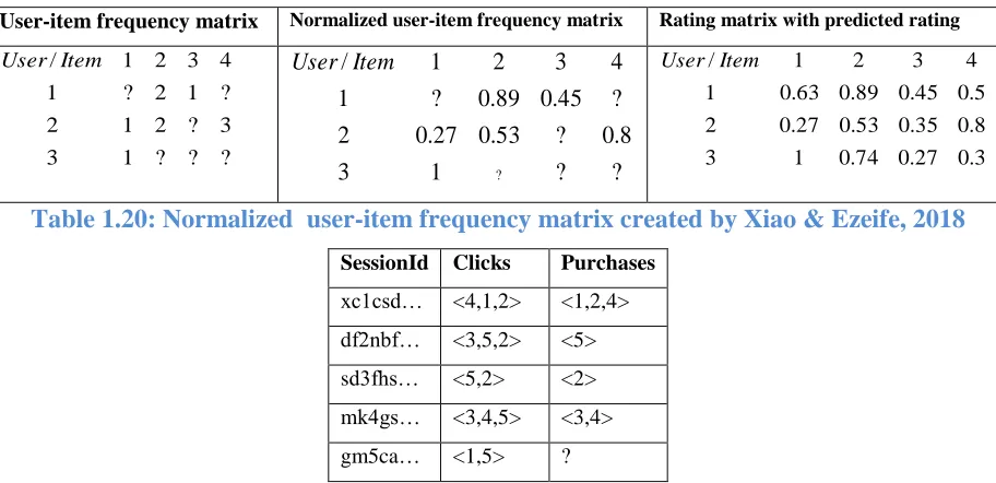
5) Historical and clickstream based recommendation- HPCRec18 (Xiao & Ezeife, 2018):

Xiao & Ezeife, 2018 proposed HPCRec18 system, which normalizes the purchase frequency matrix to improve rating quality, and mines the session-based consequential bond between clicks and purchases to generate potential ratings to improve the rating quantity. Furthermore, HPCRec18 used historical purchased frequency of item and enriched the user-item matrix from both quantity (finding the possible value for 0 rating) and quality (finding the more precise value for 1 rating) by using normalization of user-item purchase frequency matrix and using consequential bond between click and purchase. The major drawbacks of HPCRec18 are: (a) User-item matrix frequency matrix is created by neglecting sequential pattern. (b) Sequential patterns are not used in the consequential bond.

User-item frequency matrix Normalized user-item frequency matrix Rating matrix with predicted rating

? ? ? 1 3 3 ? 2 1 2 ? 1 2 ? 1 4 3 2 1 /Item User ? ? 1 3 8 . 0 ? 53 . 0 27 . 0 2 ? 45 . 0 89 . 0 ? 1 4 3 2 1 / ? Item User 3 . 0 27 . 0 74 . 0 1 3 8 . 0 35 . 0 53 . 0 27 . 0 2 5 . 0 45 . 0 89 . 0 63 . 0 1 4 3 2 1 /Item User

Table 1.20: Normalized user-item frequency matrix created by Xiao & Ezeife, 2018

SessionId Clicks Purchases xc1csd… <4,1,2> <1,2,4> df2nbf… <3,5,2> <5> sd3fhs… <5,2> <2> mk4gs… <3,4,5> <3,4> gm5ca… <1,5> ?

- 22 -

1.11.1 Summary of some close existing E-commerce recommendation systems

Existing System Methodology Input Data Limitation LiuRec09 by Liu,

Lai, &Lee, 2009

Users are first segmented by RFM. Once RFM

segmentation is created, users are further segmented with

transaction matrix. The transactions matrix contains

binary purchase information of users over a month. From

the transaction matrix, user’s purchases are further

segmented into T-2, T-1, and T, where T denotes current

purchase and T-1 and T-2 represents two previous

purchases. Finally, the association rule is used to match

Top-N neighbors from the cluster to which a target user

belongs using binary choice and derive the prediction

score of an item not yet purchased by the target user with

a frequency count of k-neighbors.

Minimum support,

historical purchase

data, and products list.

No provision for

recommending

infrequent items.

Sequential pattern

and frequency are not

considered during

recommendation.

ChoiRec12 by Choi,

Keunho, Yoo, Kim,

&Suh, 2012

Based on preference ratings from a users’ transactional

data by using the number of time useru purchased itemi

respect to total transactions. Once preference ratings are

determined, they are used to formulate a user-item rating

matrix for collaborative filtering. To a make better

recommendation, they tried to use the purchase item, but

there is no evidence of sequential purchase pattern

generated using the sequential pattern mining algorithm.

Historical purchased,

containing purchase

date and list of

purchased items.

It did not use user

purchase sequential

patterns in a user-item

matrix. Furthermore,

no provision for

making a

recommendation to

infrequent users.

SuChenRec15 by

Su & Chen, 2015

It is based on finding the common interest similarity

(frequency, duration, and path) between purchase patterns

of users to discover the closest neighbors. Frequency

similarity is computed by counting total hits occurred in

an item or category with respect to a total length of users'

browsing path. Duration similarity is computed by

considering total time spent on each category with respect

to total time spent by users'. Finally, for path similarity is

computed by counting the longest common subsequence.

Historical data

containing the

frequency of item,

path, and duration.

It requires domain

knowledge for

categories, and only

supports category

level

recommendations.

HPCRec18 by Xiao

& Ezeife, 2018

Improved the quality of user-item matrix by normalizing

the frequency of item purchase. Furthermore, they

provided the purchase possibility of clicked but not

purchased items by analysis of consequential bond.

User-item purchase

frequency and

clickstream data that

contains information’s

of click and purchase

Unable to integrate

sequential pattern

during qualitative and

quantitative analysis

- 23 - Proposed HSPRec

by Bhatta, Ezeife &

Butt, 2019

HSPRec first generates an E-Commerce sequential

database from historical purchase data using SHOD

(Sequential Historical Periodic Database Generation).

Then, mines frequent sequential purchase patterns before

using these mined sequential patterns with consequential

bonds between clicks and purchases to (i) improve the

user-item matrix quantitatively, (ii) used historical

purchase frequencies to further enrich ratings

qualitatively. Thirdly, the improved matrix is used as

input to the collaborative filtering algorithm for better

recommendations.

Minimum support,

historical purchase,

and consequential

bond of historical click

and purchase

Unable to capture

multi-database. No

provision for

infrequent user.

Table 1.22: Table showing existing E-commerce recommendations

1.12 Problem Definition

Given E-commerce historical click and purchase data over a certain period of time as input, the problem being addressed by this thesis is to find the frequent periodic (daily, weekly, monthly) sequential purchase and click patterns in the first stage. Then, these sequential purchase and click patterns can be used to make user-item matrix qualitatively (specifying level of interest or value for already rated items) and quantitatively (finding possible rating for previously unknown ratings) rich before applying collaborative filtering (CF) to improve the overall accuracy of recommendation.

1.13 Thesis Contribution