Comparison of Representations of Time Series
for Clustering Smart Meter Data
Peter Laurinec, and M´aria Luck´a
Abstract—Deployment of smart grids gives a space to emer-gence of new methods of machine learning and data analysis. Smart grids can contain of millions of smart meters, which produce large amount of data of electricity consumption. These data can be used to support intelligent grid control, make accurate forecast or to detect anomalies. The purpose of this paper is to prove that clustering of electricity consumers helps to improve accuracy of the load consumption forecast. To achieve this goal various representations of time series are compared, some of them newly proposed by us. The best results achieve data adaptive and robust model-based representation methods. We show that results of clustering can be effectively used in classifying new consumers without loss of the accuracy forecast, so there is no need of exhausting reclustering. These conclusions are evaluated on experiments made on smart meter data comming from enterprises and consumers from residences.
Index Terms—clustering, representations of time series, elec-tricity consumption, forecast.
I. INTRODUCTION
M
ORE accurate forecast methods of electricity con-sumption is an important goal, because of economic, technical and environmental reasons. This reduces the likeli-hood or even the need for excessive production of electricity, causing power control problems and environmental hazards. To achieve this goal, smart grids that consist of smart meters are employed in countries. Smart meters produce exact and fast growing data of the energy consumption. Then there is a lot of information for every customer that can be used for energy saving and improved modeling of his behavior and thus forecast improvement. In most cases, we are interested in electricity consumption of a selected larger area, thus the consumption of all customers is aggregated. Electricity consumers have generally stochastic behavior and consumers are difficult to predict individually. Therefore, the consump-tion data is aggregated (summed). For that reason, cluster analysis seems to be a suitable method for the classification of consumers to more predictable groups. Cluster analysis in the domain of energy and smart meters can also be used in other cases, namely: creation of consumer profiles, which can help by recommendation to customers to save electricity, detection of anomalies, neater monitoring of the smart grid (as a whole), emergency analysis, dynamic pricing determination for energy and the generation of more realistic synthetic data. The problem of clustering of time series of electricity consumption consists mainly of high-dimensional and noisy character of these data. This problem might beManuscript received July 19, 2016; revised July 29, 2016.
P. Laurinec and M. Luck´a are with Faculty of Informatics and Information Technologies, Slovak University of Technology in Bratislava, Ilkoviˇcova 2, 842 16 Bratislava, Slovak Republic, e-mail: [email protected] and [email protected]
solved by methods of time series data mining, which repre-sent the time series in a lower dimension. Using time series representations is appropriate from the of following reasons: reducing the dimension will reduce memory requirements and computational complexity, it implicitly removes noise and emphasizes the essential characteristics of the data. The results of cluster analysis can also be effectively used for classification of the new electricity consumers. In this paper, we focus on evidence that clustering improves accuracy of the forecast and it facilitates the classification of new customers. We work with different representations of time series that help us to achieve this goal. Some of them were taken and adapted from literature and some of them were newly proposed.
This paper is organized as follows: section 2 contains a review of the related works. In section 3 we describe data used in our experiments. Our approach is presented in section 4. Experimental evaluation and results are presented in section 5 and the conclusion is in section 5.
II. RELATEDWORK
Papers dealing with clustering of electricity consumers usually use cluster analysis primarily for two purposes. They create daily profiles of consumers with following analysis of their behavior and more accurate forecast of time series. These works, however, put little emphasis on methods of time series data mining. That is why we have focused our attention on the influence of different representations of time series, on quality of customers clustering, hence for the creation of daily profiles and on more accurate forecasts.
and Holt-Winters exponential smoothing. In paper [5] four different distance measures as the criterions of clustering of consumers are compared, namely: Euclidian, Mahalanobis, Pearson correlation and DTW (Dynamic Time Warping). Best results were achieved by the Euclidian distance and DTW, however Euclidian distance seems to be the better selection because of its stronger dependence on time.
Paper [6] deals with clustering of consumers in three different ways of feature extraction from time series and its impact on the accuracy of forecast of energy consumption. As K-means clustering method was used and neural network as a forecast method. They use three different representation of time series: estimated regression coefficients, extractions of the averages of electricity consumption and the whole time series. The best results achieved the clustering with regression coefficients, which showed significant improve-ments in the accuracy of forecast with the help of clustering. In the paper [7] are using for clustering correlation-based feature selection as representation of consumers. They want to investigate impact of aggregation on accuracy of the forecast. As forecasting methods linear regression, multi-layer perceptron and support vector regression were used.
As it was mentioned above, in the next we focus mainly on the use and influence of different representations of time series, in the context of the time series data mining. There are a several excellent review articles that examined this issue. In paper [8] detailed problems related to time series data mining and use of different representations and distance measures are decribed. Experimental and thorough comparison of the methods of representation and distance measures can be found in [9]. The authors in [10] describe in detail the use of clustering in the domain of time series for the last decade.
Our main contribution to solving selected problematic is in: a) comparison of various representation methods suitable for seasonal time series, b) several newly model-based rep-resentations of time series proposals, c) proof that clustering and advanced representation methods are improving accuracy of forecast of both residential and enterprise consumers of electricity load, d) proposal of simple and effective classifi-cation method based on the results of clustering.
III. DATA
To verify and test our approach, we used two different large data sets, comprising data from smart meters. These measurements data include Irish and Slovak data of elec-tricity consumption. Irish data were collected by the Irish Commission for Energy Regulation (CER) and are available from ISSDA1 (Irish Social Science Data Archive). These data contain three different types of customers: residential, small to medium enterprises and others. The largest group are residential, where after removing consumers with missing data, we have 3639 consumers left. The frequency of data collection was every half-hour, so in one day 48 measure-ments were performed. Slovak data were collected within the project “International Centre of Excellence for Research of Intelligent and Secure Information-Communication Tech-nologies and Systems”. These measurements are obtained mostly from Slovak enterprises (factories, etc.), having com-pletely different nature than the Irish data. After removing
[image:2.595.317.537.52.162.2]1http://www.ucd.ie/issda/data/commissionforenergyregulationcer/
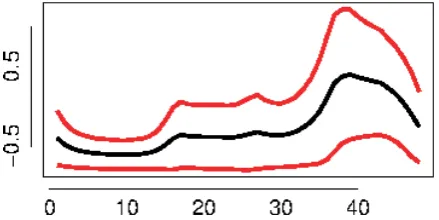
[image:2.595.317.538.200.312.2]Fig. 1. Irish median daily profile. On the vertical axis is normalized consumption and on the horizontal axis is the measurement during the day.
Fig. 2. Slovak median daily profile. On the vertical axis is normalized consumption and on the horizontal axis is the measurement during the day.
consumers with missing data and those with zero consump-tion, the customer base has size of 11281 consumers. The frequency of data collection was every quarter-hour, so in one day 96 measurements were performed. The difference between data from residences and enterprises is significant. The amount of consumption in residences is small and not quite regular, as opposed to the enterprises, where the amount of consumption can be very high and mostly regular. Enter-prise electricity consumption is therefore easier to predict, but looking for patterns in such a data can be difficult. The difference between Irish and Slovak data is visualized in Fig 1 and Fig 2, where median daily profiles (black color) with MAD deviations (red color) of Irish respectively Slovak consumers are shown. Before performing the experiment, data (consumers) were normalized using z-score.
IV. METHODOLOGY
clustering is just a simple summation of all consumers and their consumption into the one group.
A. Representations of Time Series
At the beginning we should define a time series and its representation. A Time series T [8] is an ordered sequence of nreal-valued variables
T = (x1, x2, . . . , xn), xi∈R.
Let T be a time series of length n, representation of T is a model Tˆ of reduced dimensionality d (d n) such that Tˆ closely approximates T. Changing time series on the representation makes it with suitable transformation. The main reason for the existence of representations of time series is the pursuit of more effective and easier work with time series, depending on the application. There is a large number of representations of time series, therefore, an attempt is to divide them into to the following three categories [8]: a) Nondata adaptive, b) Data adaptive and c) Model based.
In nonadaptive representations, the parameters of trans-formation remain the same for all time series, irrespective of their nature. In adaptive representations, the parameters of transformation vary depending on the available data. An approach to the model based representation relies on the assumption that the observed time series was created of some basic model. The aim is to find the parameters of such a model as a representation. Two time series are then considered as similar, if they were created by the same set of parameters of a basic model.
Based on the nature and characteristics of the available data, we will next examine and test various types of repre-sentations of given time series.
1) Nondata Adaptive Representations: The most natural representation is to use the entire time series as it is, without any transformation (we will refer as ALL). Another simple representation is PAA (Piecewise Aggregate Approxima-tion) [11]. Its idea is to replace the predetermined lengths of subsequences of time series by its average value. Formally written, the time series T of length n is represented in dimension dby vector Tˆ = (ˆx1, . . . ,xˆd). Observation i of
ˆ
T is given by the following formula:
ˆ
xi= d n
(n/d)i X
j=(n/d)(i−1)+1 xj.
In this way, other statistics from the time series can be com-puted, in addition to the average. We have not only extracted the average, but also the maximum, median and median absolute deviation (M AD=median(|Xi−median(Xi)|)).
We have created three different representations of time series, that we will now describe. The first representation was the classic PAA using the arithmetic mean (we will refer as PAA). In Slovak data the size of window was set to12and in Irish data it was set to8, so one season of measurements (96 resp.48 measured in one day) was replaced by8 resp. by 6 data (averages). The second representation was an extraction of seasonal averages and maximums, so instead of one season of measurements, the average and maximum value of the day was used (we will refer as AVE.MAX). The design of the third representation was preceded by the following data pre-processing. For each measurement xi in
Fig. 3. Comparison of PAA and PLA representation on a randomly picked Irish consumer. On the vertical axis is normalized consumption and on the horizontal axis is the measurement during the day.
the time series the median absolute deviation was calculated. It means thatndeviations of all consumers were calculated and the first quartile Q1 for these data was determined. If the deviation was less than the first quartile, then the measurement was evaluated as not enough variable and as carrying too little information. From this analysis of variance a frequency table of smallest deviating measurements during the day was obtained. The results showed that the least deviate measurements from the median placed at the start and at the very end of the day. Therefore these measurements were removed from each day of the data set, resulting in the removing of28, resp.12measurements in the Slovak, resp. Irish data. From these adjusted data three seasonal statistics were extracted: seasonal median, maximum and median variation (we will refer as MMM) - that is the same idea as in the second representation with average and maximum. Another very common technique used to represent time series is the Discrete Wavelet Transform (ref. DWT) [12]. It is a technique of the decomposition of the signal. Wavelets are mathematical functions that represent data in terms of sums and differences of the so called prototype functions, or in the other words the mother wavelets. The simplest wavelet is the Haar wavelet, which was also used in our comparisons. The level of averaging coefficients was opted to5, respectively
4, for the Slovak data, resp. for Irish data. It means that the time series dimension was reduced25-times, respectively24 -times.
2) Data Adaptive Representations: Here the well-known adaptive method of representation PLA (Piecewise Lin-ear Approximation (we will refer as PLA)) was imple-mented [13]. It is a method of segmentation of time series, which approximates the time series by straight lines. PLA is a bottom-up type of algorithm. It begins by creating a simple approximation of the time series, i.e.n/2segments are used and then iteratively connects pairs of segments with the least losses, until it reaches to the given number of segments. The number of segments (the number of points of representation), was chosen to the(number of days×2). In Fig 3 is shown difference between PAA and PLA representation.
3) Model-based Representations: Another group of rep-resentations of time series are methods based on a model. These representations are mostly present in this paper, be-cause of the seasonal nature of our data. In one season (1
[image:3.595.308.546.53.151.2]season as seas. Then the number of points in the model-based representation of seasonal time series is also seas,
ˆ
T = (ˆx1, . . . ,xseasˆ ). In the next we will present three
regression based methods. The first representation is based on the multiple linear regression (we will refer as LM). Similar as other regression methods it aims to model the dependent variable by independent variables. Formally, the model will be written as follows:
xi=β1ui1+β2ui2+· · ·+βseasuiseas+εi, (1)
for i = 1, . . . , n, where ui is the i−th electricity con-sumption, β1, . . . , βseas are the regression coefficients. The ui1, . . . , uiseas are independent binary (dummy) variables
representing the sequence numbers in regression model. That equals1just in the case when they point to thej−thvalue of the season,j= (1,2, . . . , seas). Theεi is a random error with the normal distribution ofN(0, σ2)and are independent. The most widespread method for obtaining an estimate of the vectorβ= (β1, . . . , βseas)is the ordinary least squares
(OLS). Another representation method is the robust linear regression (we will refer as RLM). From the classical linear regression it differs by parameter estimation, so the model is identical to the Eq. 1. One of the robust parameter estimation methods is M-estimate [14]. This method is robust towards errors, which have a distribution with heavy tails and towards outliers in the vector x. Its idea is to minimize errors with some slower increasing function when compared with the sum of squares. We have used the ψ-Huber function. The estimation of the vectorβis then calculated using re-iterated weighted least squares (IRLS). Possible extension for linear models is the generalized additive model (we will refer as GAM) [15]. The difference when compared to the multiple linear regression is that the variables (predictors) are modeled by using the smoothing functions. The model can be written as follows:
E(xi) =β0+f1(ui1), i= 1, . . . , n,
where f1 is a cyclic cubic regression spline and u1 is the
vector of type(1,2, . . . , seas,1, . . . , seas, . . .). The param-eters of the model are estimated by penalized iteratively re-weighted least squares (P-IRLS).
Holt-Winters exponential smoothing was used as another method of representation based on the model. It is a method that is used mainly to forecast the seasonal time series and to smoothing time series from the noise [16]. Components of the triple (with trend and seasonality) exponential smoothing are:
li=α(xi−st−seas) + (1−α)(li−1+bi−1) bi=β(li−li−1) + (1−β)bi−1
si=γ(xi−li−1−bt−1) + (1−γ)si−seas, i= 1, . . . , n,
where l is smoothing component, b is trend component, s
is seasonal component, α, β and γ are smoothing factors. We have computed exponential smoothing without trend component b. As representation, we then took the following seasonal coefficientss,Tˆ= (sn−seas+1, sn−seas+2, . . . , sn).
Smoothing factors have been selected in two ways, thus two different representations were created. The first method was manual (we will refer as HW), where the factors were set to
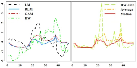
[image:4.595.306.546.52.171.2]α= 0.15andγ= 0.95. The second method was automated (we will refer as HW-auto), where the factors were optimized
Fig. 4. Comparison of seven mode-based representations. On the vertical axis is normalized consumption and on the horizontal axis is the measure-ment during the day.
according to the average square error of the one-stepwise prediction. The last two representations were average, re-spectively median, daily consumer profiles (we will refer as Average resp. Median). Point of the representation xkˆ ,
k= (1, . . . , seas),dis the number of days in the data set, is calculated as follows:
ˆ
xk = 1
d d−1 X
j=0
xk+seas×j
ˆ
xk =median((xk, xk+seas, . . . , xk+seas×(d−1))).
In Fig 4 comparisons of seven differnt model-based represen-tations on randomly picked Irish consumer data are shown. Table I summarized all the representation of time series.
TABLE I
CLASSIFICATION OF REPRESENTATIONS OF TIME SERIES USED IN OUR EXPERIMENTS.
Type Acronym
Nonadadptive ALL, PAA, AVE.MAX, MMM, DWT
Adaptive PLA
Model based LM, RLM, GAM, HW, HW-auto, Average, Median
B. Cluster Analysis
For classification consumers into groups (clusters), we used the centroid based clustering method K-means [17]. K-means is a method based on the mutual distances of objects, measured by Euclidean distance. We have compared K-means with the K-medoids method experimentally, and concluded that the K-means gave better results. In the next just results using K-means method are presented. Before applying the K-means algorithm the optimal number of clusters k must be determined. For each representation of a data set, we have determined the optimal number of clusters tokusing the internal validation rate Davies-Bouldin index [18]. The optimal number of clusters ranged from10
to15.
C. Classification
distance. Then the centroid (arithmetic average of all con-sumers in the cluster) is updated incrementally. This method is also computationally inexpensive, because it consists only of calculating the distances between the representation of time series of a new consumer andk centroids followed by the centroid update.
D. Time Series Forecast
To confirm the hypothesis that clustering improves forecast accuracy, we used three methods for time series forecast. Support vector regression (SVR), a method based on a com-bination of STL decomposition and Holt-Winters exponential smoothing and ARIMA model. Support vector regression is a method often used in the forecast of seasonal time series [19] [20]. In our experiments, epsilon regression with Gaussian RBF kernel was used. Seasonal decomposition of time series based on loess regression (STL) is a method, which decomposes seasonal time series into three parts: trend, seasonal component and remainder (noise) [21]. For the final three time series any of the forecast methods is used separately, in our case either Holt-Winters exponential smoothing or ARIMA model. ARIMA model was introduced by Box and Jenkins [22] and it is one of the most used approaches for predicting time series [23]. The model is com-posed of three parts: autoregression (AR), moving average (MA) and differential process. In the case of non-stationary random process, it is important transform it to the stationary time series. This is done in the model by differentiating the original series.
The accuracy of the forecast of electricity consumption was measured by MAPE (Mean Absolute Percentage Error). MAPE is defined as follows:
MAPE= 100×1 n
n X
t=1
|xt−xt| xt ,
wherextis a real consumption,xtis a forecasted load and
nis a length of the time series.
V. EVALUATION ANDEXPERIMENTS
Experimental evaluation of decribed methods was per-formed on three data sets. The first one was created as a comparison to the [6]. It covers the Irish data from the period of 1st February 2010 to 7th March 2010. The second data set from Ireland has a range from 2nd September 2010 to 11th October 2010, the same range has the Slovak data set, with the only difference that the measurements were made in the year 2013. The forecast methods were always trained on a window of ten days of Mondays to Fridays because of the similarity of consumption during these days. Prediction was calculated always one day ahead. Prediction of the next day is then carried out so that the window is shifted by one day, i.e. the first day of the window is removed and current day is added. As mentioned above, the accuracy of the prediction was calculated using the MAPE.
Verification of success of clustering and classification was done by random sampling of consumers from the data set. For the Irish data there was randomly selected always3400
from 3639 consumers, of which 300 have been previously classified as described in Section IV-C. For the Slovak data there was randomly selected always10800from11281
consumers, of which 300 was previously classified. This process was always performed100times and then the results were averaged.
In addition to a comparison of average deviations of MAPE we have compared our three approaches tested also with the Wilcoxon rank sum test [24]. We wanted to confirm a hyphotesis whether clustering together with the classifica-tion has significantly the same accuracy of forecast as it has the forecast itself with clustering. Second hyphotesis con-cerned fact that forecast used with clustering is significantly more accurate than forecasts of aggregate consumption. The Wilcoxon rank sum test is a version of the non-parametric two-sample t-test. We used it because of the fact that the distribution of prediction errors is not normally distributed (tested with Shapiro-Wilk test [25] and Q-Q plot).
In Table II the results of experiments comparing all thirteen defined representations of time series and the three aggregation method of forecast are showed. The results in the table are the average MAPE for the three forecast methods of time series (SVR, STL decomposition together with Holt-Winters and STL with ARIMA model). P-values of Wilcoxon rank sum test came out positive in terms of our hypothesis in all cases except non-adaptive representations (ALL, PAA, AVE.MAX, MMM and DWT) on Slovak data. The forecast associated with clustering was, except for that case, always significantly more accurate than the forecast of aggregate consumption. Forecast accuracy associated with the classifi-cation was significantly the same as the forecast associated with clustering. This implies that the clustering of consumers improves accuracy of forecast of electricity consumption. In case of February’s Irish data and the best representation PLA, it is accurate by0.6293%, in the case of September’s Irish data and the best representation PLA, it is accurate by
0.6645% and in the case of the September’s Slovak data and best representation HW-auto it is accurate by0.1563%. Results also showed that the classification of new consumers will not adversely affect the accuracy of forecast. The best results were achieved by model based representations and adaptive method PLA. For Ireland data the best represen-tation was the PLA. Very good results were achieved with robust representations like the RLM and the median daily profile. Consistently good results have also been obtained by the representation based on the Holt-Winters exponential smoothing with manual parameter settings. On the contrary, non-adaptive methods have not been a success at all. We have also observed how the size of consumer base (number of consumers in the model) is affecting accuracy of forecast associated with clustering and aggregate consumption. In Fig 5 the results of this experiment, performed on the Slovak data and representation of Median are illustrated. It was confirmed that the bigger the base of consumers is, the more accurate forecast based on clustering is.
VI. CONCLUSION
TABLE II
RESULTS OF EXPERIMENTS INMAPE. CLASSIF.MEANS FORECAST ASSOCIATED WITH CLASSIFICATION AND CLUSTERING, CLUSTER.IS
ASSOCIATED WITH THE FORECAST WITH CLUSTERING, AGG.IS THE FORECAST OF AGGREGATE CONSUMPTION. IN BOLD THE THREE BEST
RESULTS OF FORECAST WITH CLUSTERING ARE SHOWN.
Repres. Ireland - February Ireland - September Classif. Clus. Agg. Classif. Clus. Agg. All 4.0488 4.0424 4.5055 5.0342 5.0360 5.4692 PAA 4.0408 4.0482 4.5197 4.9840 4.9907 5.4308 AVE.MAX 4.0649 4.0681 4.5099 5.0861 5.1002 5.4897 MMM 4.1054 4.0986 4.5108 5.1267 5.1404 5.4785 DWT 4.0867 4.0775 4.4903 5.0134 5.0220 5.4283 PLA 3.9248 3.9213 4.5506 4.7555 4.7603 5.4248 LM 4.0215 4.0185 4.5091 5.0542 5.0539 5.4745 RLM 3.9234 3.9176 4.5077 4.9004 4.9053 5.4222 GAM 3.9233 3.9238 4.4961 5.0132 5.0193 5.4716 Average 3.9571 3.9522 4.4888 5.0336 5.0256 5.4721 Median 3.9462 3.9497 4.5237 4.8932 4.8901 5.4160 HW 3.9215 3.9168 4.5208 4.9424 4.9439 5.4817 HW-auto 3.9368 3.9391 4.4927 5.1763 5.1722 5.4706
[image:6.595.293.548.104.767.2]Repres. Slovak - September Classif. Clus. Agg. All 3.0145 3.0250 2.8766 PAA 3.0200 3.0206 2.8767 AVE.MAX 2.9779 2.9773 2.8839 MMM 2.9189 2.9255 2.8668 DWT 2.9760 2.9751 2.8638 PLA 2.7365 2.7369 2.8614 LM 2.7319 2.7281 2.8758 RLM 2.7396 2.7405 2.8598 GAM 2.7514 2.7531 2.8930 Average 2.7431 2.7435 2.8829 Median 2.7150 2.7164 2.8541 HW 2.7258 2.7196 2.8768 HW-auto 2.7117 2.7155 2.8718
Fig. 5. The impact of the size of the customer base to forecast accuracy.
clustering can improve forecast accuracy and to compare different representations of time series. In this regard, we used representation methods that have been not used before. These representations were based on model, such as robust linear regression, generalized additive model, Holt-Winters exponential smoothing and the median daily profile. We have shown that the best representations in this task are adap-tive representations (PLA) and model-based representations, particularly the robust ones (RLM and Median). We have found a method for classification of new consumers, which has proved to be successful and which does not worsen the accuracy of forecast.
ACKNOWLEDGMENT
This work was partially supported by the Research and Development Operational Programme for the project “In-ternational Centre of Excellence for Research of Intelligent and Secure Information-Communication Technologies and
Systems”, ITMS 26240120039, co-funded by the ERDF and the Scientific Grant Agency of The Slovak Republic, grant No. VG 1/0752/14 .
REFERENCES
[1] S. Haben, C. Singleton, P. Grindrod, “Analysis and Clustering of Residential Customers Energy Behavioral Demand Using Smart Meter Data,” in Smart Grid, IEEE Transactions on, vol.PP, no.99, pp.1-9, 2015.
[2] J. D. Rhodes, W. J. Cole, Ch. R. Upshaw, T. F. Edgar, M. E. Webber, “Clustering analysis of residential electricity demand profiles,”Applied Energy, Volume 135, Pages 461-471, 2014.
[3] T. Rsnen, M. Kolehmainen, “Feature-based clustering for electricity use time series data,”In Proceedings of the 9th international conference on Adaptive and natural computing algorithms, Springer-Verlag, Berlin, Heidelberg, pp.401-412, 2009.
[4] D. Ili, P. G. da Silva, S. Karnouskos, M. Jacobi, “Impact assessment of smart meter grouping on the accuracy of forecasting algorithms,”In Proceedings of the 28th Annual ACM Symposium on Applied Computing (SAC), pp.673-679, 2013.
[5] F. Iglesias, W. Kastner, “Analysis of Similarity Measures in Times Series Clustering for the Discovery of Building Energy Patterns,”
Energies, vol.6, pp.579-597, 2013.
[6] A. Shahzadeh, A. Khosravi, S. Nahavandi, “Improving load forecast accuracy by clustering consumers using smart meter data,”International Joint Conference on Neural Networks (IJCNN), pp. 1-7, 2015. [7] T. K. Wijaya, M. Vasirani, S. Humeau, K. Aberer, “Cluster-based
Aggregate Forecasting for Residential Electricity Demand using Smart Meter Data,”In proceedings of IEEE International Conference on Big Data, 2015.
[8] P. Esling, C. Agon, “Time-Series data mining,”ACM Comput. Surv., vol.45, 2012.
[9] X. Wang, et. al., “Experimental comparison of representation methods and distance measures for time series data,”Data Mining and Knowl-edge Discover, vol. 26, iss. 2, pp. 275309, 2013.
[10] S. Aghabozorgi, A. S. Shirkhorshidi, T. Y. Wah, “Time-series cluster-ing A decade review,”Information Systems, vol. 53, pp. 16-38, 2015. [11] E. Keogh, K. Chakrabarti, M. Pazzani, Sh. Mehrotra, “Dimensionality Reduction for Fast Similarity Search in Large Time Series Databases,”
Knowledge and Information Systems, vol. 3, n.3, pp. 263-286, 2001. [12] K. P. Chan, A. W.-Ch. Fu, “Efficient time series matching by wavelets,”
Data Engineering, 1999. Proceedings., 15th International Conference on, Sydney, NSW, pp. 126-133, 1999.
[13] Y. Zhu, D. Wu, Sh. Li, “A Piecewise Linear Representation Method of Time Series Based on Feature Points,”Knowledge-Based Intelligent Information and Engineering Systems, vol. 4693 of the series Lecture Notes in Computer Science, pp. 1066-1072, 2007.
[14] R. Andersen, “Modern Methods for Robust Regression,” 152. edition,
SAGE Publications, 2008.
[15] S. N. Wood, “Generalized Additive Models: An Introduction with R,” Chapman & Hall/CRC., 2006.
[16] R. J. Hyndman, A. B. Koehler, R. D. Snyder, S. Grose, “A state space framework for automatic forecasting using exponential smoothing methods,” International Journal of Forecasting, vol. 18, issue 3, pp. 439-454, 2002.
[17] A. K. Jain, “Data clustering: 50 years beyond K-means,”Pattern Recognition Letters, vol. 31, Issue 8, pp. 651-666, 2009
[18] D. L. Davies, D. W. Bouldin, “A cluster separation measure,”IEEE Transactions on Pattern Analysis and Machine Intelligence, PAMI-1, no.2, pp.224-227, 1979.
[19] Ch. N. Ko, Ch. M. Lee, “Short-term load forecasting using SVR (support vector regression)-based radial basis function neural network with dual extended Kalman filter,”Energy, vol. 49, pp. 413-422, 2013. [20] J. X. Che, J. Z. Wang, “Short-term load forecasting using a kernel-based support vector regression combination model,”Applied Energy, vol. 132, pp. 602-609, 2014.
[21] R. B. Cleveland, et. al., “Seasonal-Trend Decomposition Procedure based on LOESS,”J. Official Stat., vol. 6, pp. 3-73, 1990.
[22] G. E. P. Box, G. M. Jenkins, “Time Series Analysis: Forecasting and Control,” San Francisco, CA: Holden-Day, 1970.
[23] W. C. Hong, “Intelligent Energy Demand Forecasting,” London: Springer Verlag, 2013.
[24] M. Hollander, et. al., “Nonparametric Statistical Methods,” Hoboken, NJ: J. Wiley & Sons, 2014.