A Bayesian view on acoustic model based techniques for robust speech recognition

R E V I E W

Open Access

A Bayesian view on acoustic model-based

techniques for robust speech recognition

Roland Maas

, Christian Huemmer

, Armin Sehr

and Walter Kellermann

Abstract

This article provides a unifying Bayesian view on various approaches for acoustic model adaptation, missing feature, and uncertainty decoding that are well-known in the literature of robust automatic speech recognition. The

representatives of these classes can often be deduced from a Bayesian network that extends the conventional hidden Markov models used in speech recognition. These extensions, in turn, can in many cases be motivated from an underlying observation model that relates clean and distorted feature vectors. By identifying and converting the observation models into a Bayesian network representation, we formulate the corresponding compensation rules. We thus summarize the various approaches as approximations or modifications of the same Bayesian decoding rule leading to a unified view on known derivations as well as to new formulations for certain approaches.

Keywords: Robust automatic speech recognition, Bayesian network, Model adaptation, Missing feature, Uncertainty decoding

1 Introduction

Robust automatic speech recognition (ASR) still repre-sents a challenging research topic. The main obstacle, namely the mismatch of test and training data, can be tackled by enhancing the observed speech signals or fea-tures in order to meet the training conditions or by com-pensating for the distorted test conditions in the acoustic model of the ASR system.

Methods that modify the acoustic model are in general termed (acoustic) model-based or model compensation approaches and comprise inter alia the following sub-categories: so-calledmodel adaptationtechniques mostly update the parameters of the acoustic model, i.e., of the hidden Markov models (HMMs), prior to the decod-ing of a set of observed feature vectors. In contrast, decoder-based approaches re-adapt the HMM parame-ters for each observed feature vector. The most common decoder-based approaches aremissing featureand uncer-tainty decoding that incorporate additional time-varying uncertainty information into the evaluation of the HMMs’ probability density functions (pdfs).

*Correspondence: [email protected]

1Multimedia Communications and Signal Processing, University of Erlangen-Nuremberg, Cauerstr. 7, 91058 Erlangen, Germany Full list of author information is available at the end of the article

Various model compensation techniques exhibit two (more or less) distinct steps: First, the compensation parameters need to be estimated and, second, the actual compensation rule is applied to the acoustic model. The compensation rules can often be motivated based on an observation model that relates the clean and distorted fea-ture vectors, e.g., in the logarithmic melspectral (logmel-spec) or the mel frequency cepstral coefficient (MFCC) domain.

In this article, we review and examine for several uncer-tainty decoding [1–5], missing feature [6–9], and model adaptation techniques [10–19] how their compensation rules can be formulated as an approximated or mod-ified Bayesian decoding rule. In order to illustrate the formalism, we also present the corresponding Bayesian network representations. In addition to the above tech-niques, we give a Bayesian network description of the generic uncertainty decoding approach of [20], of the maximum a posteriori (MAP) adaptation technique [21], and of some alternative HMM topologies [22, 23]. While the Bayesian perspective [24, 25] and Bayesian networks have been employed in this context before [4, 9, 20], with this article, we present new formulations for certain of the considered algorithms in order to fill some gaps for a unified description. Throughout the following, feature

vectors are column vectors and denoted by bold-face let-ters vn with time indexn ∈ {1,. . .,N}. Feature vector sequences are written asv1:N = (v1,. . .,vN). The

oper-ators “exp” and “log” applied to vectors are meant to be applied component-wise. The operator “” denotes the component-wise vector multiplication (Hadamard prod-uct). Without distinguishing a random variable from its realization, a pdf over a random variableznis denoted by p(zn). For a normally distributed real-valued random vec-torzn with mean vectorμzn and covariance matrixCzn,

we writezn∼N(μzn,Czn)or

p(zn)=N(zn;μz_n,Czn). (1)

To express that all random vectors of the set{z1,. . .,zN}

share the same statistics, we writep(zn)=const. or in the Gaussian case,

p(zn)=N(zn;μz,Cz) (2)

with time-invariant mean vector μz and covariance matrixCz. Finally, for a Gaussian random vectorzn

con-ditioned on another random vectorwn, we write

p(zn|wn)=N(zn;μz|wn,Cz|wn), (3)

if the statistics ofzndepend only on time throughwn, i.e., ifμz_|wn = μz|wm andCz|wn = Cz|wm forwn = wmand

n,m∈ {1,. . .,N}.

The remainder of the article is organized as fol-lows: After summarizing the employed Bayesian view in Section 2 and its difference to other overview articles in Section 3, this perspective is applied to uncertainty decoding, missing feature techniques, and other model-based approaches in Sections 4, 5, and 6, respectively. In Section 7, we point out the relation of the presented techniques to deep learning-based architectures. Finally, conclusions are drawn in Section 8.

2 The Bayesian view

We start by reviewing the Bayesian perspective on acous-tic model-based techniques that we use in Sections 4, 5, 6, and 7 to review different algorithms.

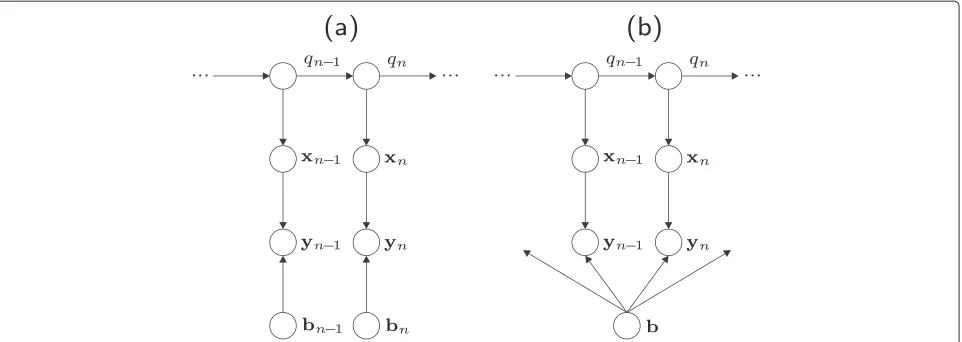
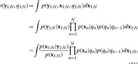
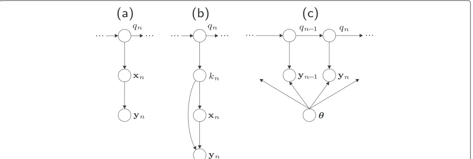
Given a sequence of observed feature vectorsy1:N, the acoustic scorep(y1:N|W)of a sequencewof conventional HMMs, as depicted in Fig. 1a, is given by [24]

p(y1:N|W) =

q1:N

p(y1:N,q1:N) (4)

=

q1:N

_N

n=1

p(yn|qn)p(qn|qn−1)

, (5)

where p(q1|q0) = p(q1). The summation goes over all

possible state sequencesq1:N throughWsuperseding the

explicit dependency on wat the right-hand side of (4) and (5). Note that the pdfp(yn|qn)can be scaled byp(yn) without influencing the discrimination capability of the acoustic score w.r.t. changing word sequencesw. We thus definep˚(yn|qn)=p(yn|qn)/p(yn)for later use.

The compensation rules of a wide range of model adaptation, missing feature, and uncertainty decoding approaches can be expressed by modifying the Bayesian network structure of a conventional HMM and applying the inference rules of Bayesian networks [26]—potentially followed by suitable approximations to ensure mathemati-cal tractability. While some approaches postulate a certain Bayesian network structure, others indirectly define a modified Bayesian network by assuming an observed fea-ture vectoryn to be adistortedversion of an underlying cleanfeature vectorxn, which is introduced as latent vari-able in the HMM as, e.g., in Fig. 1b. In the latter case, the relation of yn and xn can be expressed by an ana-lytical observation model g(·) that incorporates certain compensation parametersbn:

yn=g(xn,bn). (6)

Note that here it is not distinguished whetherynis the output of a front-end enhancement process or a noisy or reverberant observation that is directly fed into the recognizer. By converting the observation model to a Bayesian network representation, the pdfp(yn|qn)in (5) can be derived exploiting the inference rules of Bayesian networks [26]. For the case of Fig. 1b, the observation likelihood in (5) would, e.g., become:

p(yn|qn) =

p(xn,yn|qn)dxn

=

p(xn|qn)p(yn|xn)dxn, (7)

where the actual functional form ofp(yn|xn)depends on the assumptions ong(·)and the statisticsp(bn)ofbn.

The abstract perspective taken in this paper reveals a fundamental difference between model adaptation approaches on the one hand and missing feature and uncertainty decoding approaches on the other hand: Model adaptation techniques usually assumebn to have constant statistics over time [4, 27], i.e.,

p(bn)=const., forn∈ {1,. . .,N}. (8)

or to be a deterministic parameter vector of valueb, i.e.,

p(bn)=δ(bn−b), (9)

Fig. 1Bayesian network representation ofaa conventional HMM andban HMM incorporating latent feature vectors. Subfigurebis based on [20]

As exemplified in Sections 4 to 6, this Bayesian view also allows for a convenient illustration of the underly-ing statistical dependencies of model-based approaches by means of Bayesian networks. If two approaches share the same Bayesian network, their underlying joint pdfs over all involved random variables share the same decompo-sition properties. However, some crucial aspects are not reflected by a Bayesian network: the particular functional form of the joint pdf, potential approximations to arrive at a tractable algorithm, as well as the estimation procedure for the compensation parameters. While some approaches estimate these parameters through an acoustic front-end, others derive them from clean or distorted data. For clar-ity, we entirely focus in this article on the compensation rules while ignoring the parameter estimation step. We also disregard approaches that apply a modified training method to conventional HMMs without exhibiting a dis-tinct compensation step, as it is characteristic for, e.g., discriminative [28], multi-condition [29], or reverberant training [30].

3 Merit of the Bayesian view

In the past decades, numerous survey papers and books have been published summarizing the state-of-the-art in noise and reverberation-robust ASR [27, 31–36]. Recently, a comprehensive review of noise-robust ASR techniques was published in [25] providing a taxonomy-oriented framework by distinguishing whether, e.g., prior knowl-edge, uncertainty processing or an explicit distortion model is used or not. In contrast to [25] and previous survey articles, we pursue a threefold goal with this article:

• First of all, we aim at classifying all considered techniques along the same dimension by motivating and describing them with the same Bayesian formalism. Consequently, we do not conceptually distinguish whether a given method employs a time-varying pdfp(bn), as in uncertainty decoding, or

whether a distorted vectorynis a preprocessed or a

genuinely noisy or reverberant observation. Also, the distinction of implicit and explicit observation models dissolves in our formalism.

• As a second goal, we aim at closing some gaps by presenting new derivations and formulations for some of the considered techniques. For instance, the Bayesian networks in Figs. 2b, 2c, 4, 5b, 5c, 6b, 8, 9b representing the concepts in Subsections 4.3, 4.4, 4.6, 6.3/6.4, 6.5, 6.6, 6.8, and 6.9, respectively, constitute novel representations. Moreover, the links to the Bayesian framework via the mathematical

reformulations in (28), (29), (37), (38), (45), (55), (61), (65), (71) are explicitly stated for the first time in this paper.

• The third goal of the Bayesian description is to provide an intuitive graphical illustration that allows to easily overview a broad class of algorithms and to immediately identify their similarities and differences in terms of the underlying statistical assumptions.

By establishing new links between existing concepts, such an abstract overview should therefore also serve as a basis for revealing and exploring new directions. Note, however, that the review presented in this paper does not claim to cover all relevant acoustic model-based tech-niques and is rather meant as an inspiration to other researchers.

4 Uncertainty decoding

In the following, we consider the compensation rules of several uncertainty decoding techniques from a Bayesian view.

4.1 General example of uncertainty decoding

A fundamental example of uncertainty decoding can, e.g., be extracted from [1, 37–42]. The underlying observation model can be identified as

yn=xn+bnwithbn∼N(0,Cbn), (10)

where yn and Cbn often play the role of an enhanced

Fig. 2Bayesian network representation of different model compensation techniques. Detailed descriptions of subfiguresatodare given in the text. Subfiguredis based on [4]

be seen as being enriched by the additional reliability informationCbn. The observation model is representable

by the Bayesian network in Fig. 2a. Exploiting the con-ditional independence properties of Bayesian networks [26], the compensation of the observation likelihood in (5) leads to [26]

p(yn|qn) =

p(xn|qn)p(yn|xn)dxn

=

N(xn;μx|qn,Cx|qn)N(yn;xn,Cbn)dxn

= N(yn;μx_|qn,Cx|qn+Cbn). (11)

Without loss of generality, a single Gaussian pdf p(xn|qn) is assumed since, in the case of a Gaussian mixture model (GMM), the linear mismatch function (10) can be applied to each Gaussian component separately.

4.2 Dynamic variance compensation

The concept of dynamic variance compensation [2] is based on a reformulation of the log-sum observation model [39]:

yn=xn+log(1+exp(rn−xn))+bn (12)

withrnbeing a noise estimate of any noise tracking algo-rithm andbn∼N(0,Cbn)a residual error term. Since the

analytical derivation ofp(yn|qn)is intractable, an approxi-mate pdf is evaluated based on the assumption ofp(xn|yn) being Gaussian and that the compensation can be applied to each Gaussian component of the GMM separately [2].

According to Fig. 2a, the observation likelihood in (5), in its scaled versionp˚(yn|qn), hence becomes:

˚

p(yn|qn) =

p(xn|qn)

p(xn|yn) p(xn)

dxn

≈

p(xn|qn)p(xn|yn)dxn (13)

≈

N(xn;μx_|qn,Cx|qn)N(xn;μx|yn,Cx|yn)dxn

= N(μx|qn;μx|yn,Cx|qn+Cx|yn), (14)

where the approximation (13) can be justified if p(xn)is assumed to be significantly “flatter,” i.e., of larger variance, thanp(xn|yn). The estimation of the momentsμx_|yn,Cx|yn

ofp(xn|yn)represents the core of [2].

4.3 Uncertainty decoding with SPLICE

The stereo piecewise linear compensation for environ-ment (SPLICE) approach, first introduced in [43] and further developed in [44, 45], is a popular method for cep-stral feature enhancement based on a mapping learned from stereo (i.e., clean and noisy) data [25]. While SPLICE can be used to derive an minimum mean square error (MMSE) [44] or MAP [43] estimate that is fed into the rec-ognizer, it is also applicable in the context of uncertainty decoding [3], which we focus on in the following. In order to derive a Bayesian network representation of the uncer-tainty decoding version of SPLICE [3], we first note from [3] that one fundamental assumption is

where sn denotes a discrete region index, rsn is its bias,

and sn the uncertainty in that region. Exploiting the

symmetry of the Gaussian pdf

p(xn|yn,sn) = N(xn;yn+rsn,sn)

= N(yn−xn;−rsn,sn) (16)

and definingbn = yn −xn, we identify the observation model to be

yn=xn+bn (17)

given a certain region indexsn. In the general case ofsn depending onxn, the observation model can be expressed by the Bayesian network in Fig. 2b with

p(bn|sn)=N(bn;−rsn,sn). (18)

This reveals that the introduction of different regionssn is equivalent to assuming an affine model (18) withp(bn) being a GMM instead of a single Gaussian density, as in (10). By introducing a separate prior model

p(yn) = sn

p(sn)p(yn|sn)

=

sn

p(sn)N(yn;μy|sn,Cy|sn), (19)

for the distorted speechyn, the likelihood in (5) can be adapted according to

p(yn|qn)=

p(xn|qn)p(yn|xn)dxn

=

p(xn|qn)

p(xn,yn) p(xn) dxn=

p(xn|qn)

·

snp(xn|yn,sn)p(yn|sn)p(sn)

sn p(xn|yn,sn)p(yn|sn)p(sn)dyn

dxn.

(20)

Although analytically tractable, both the numerator and the denominator in (20) are typically approximated for the sake of runtime efficiency [3].

4.4 Joint uncertainty decoding

Model-based joint uncertainty decoding [4] assumes an affine observation model in the cepstral domain

yn=Aknxn+bn (21)

with the deterministic matrix Akn and p(bn|kn) =

N(bn;μb_|kn,Cb|kn)depending on the considered Gaussian

componentknof the GMM of the current HMM stateqn:

p(xn|qn)=

kn

p(kn)p(xn|kn). (22)

The Bayesian network is depicted in Fig. 2c implying the following compensation rule:

p(yn|kn)=

p(xn|kn)p(yn|xn,kn)dxn, (23)

which can be analytically derived analogously to (11). In practice, the compensation parameters Akn, μb|kn, and

Cb|kn are not estimated for each Gaussian componentkn

but for each regression class comprising a set of Gaussian components [4].

4.5 REMOS

As many other techniques, the reverberation modeling for speech recognition (REMOS) concept [5, 46] assumes the environmental distortion to be additive in the melspectral domain. However, REMOS also considers the influence of the L previous clean speech feature vectors xn−L:n−1

in order to model the dispersive effect of reverberation and to relax the conditional independence assumption of conventional HMMs. The observation model reads in the logmelspec domain:

yn = log

exp(cn)+exp(hn+xn)

+exp(an) L

l=1

exp(μl+xn−l)

, (24)

where the normally distributed random variables cn,hn, and an model the additive noise components, the early part of the room impulse response (RIR), and the weight-ing of the late part of the RIR, respectively, and the parametersμ1:_L represent a deterministic description of the late part of the RIR. The Bayesian network is depicted in Fig. 3 with bn =[cn,an,hn]. In contrast to most of the other compensation rules reviewed in this article, the REMOS concept necessitates a modification of the Viterbi decoder due to the introduced cross-connections in Fig. 3.

In order to arrive at a computationally feasible decoder, the marginalization over the previous clean speech com-ponentsxn−L:n−1is circumvented by employing estimates

xn−L:n−1(qn−1)that depend on the best partial path, i.e.,

on the previous HMM state qn−1. The resulting

analyt-ically intractable integral is then approximated by the maximum of its integrand:

The determination of a global solution to (25) repre-sents the core of the REMOS concept. The estimates xn−L:n−1(qn−1)in turn are the solutions to (25) at previous

time steps. We refer to [5] for a detailed derivation of the corresponding decoding routine.

It seems worthwhile noting that the simplification in (25) represents a variant of the MAP integral approxima-tion, as often applied in Bayesian estimation [26]. To show this, we first omit the dependency onxn−L:n−1(qn−1)for

where we scaled the objective function in the second step by the constant 1/p(yn|qn). We can now reformu-late the Bayesian integral leading to a novel derivation of (25)

We see that the assumption underlying (25) is a modified MAP approximation:

which slightly differs from the conventional MAP approximation:

The obvious disadvantage of (29) is that the resulting score (25) does not represent a normalized likelihood w.r.t. toyn. On the other hand, the modified MAP approxima-tion (29) leads to a scaled version of the exact likelihood p(yn|qn), cf. (27), with the scaling factor p(xMAPn |yn,qn) being all the higher with increasing accuracy of the approximation (29).

4.6 Ion and Haeb-Umbach

Similarly to REMOS, the generic uncertainty decoding approach given in [24], and first proposed by [20], con-siders cross-connections in the Bayesian network in order to relax the conditional independence assumption of HMMs. The concept, as described in [24], is an example of uncertainty decoding, where the compensation rule can be defined by a modified Bayesian network structure— given in Fig. 4a—without fixing a particular functional form of the involved pdfs via an analytical observation model. In order to derive the compensation rule, we start by introducing the sequence x1:N of latent clean speech vectors in each summand of (4)

p(y1:N,q1:N)=

where we exploited the conditional independence proper-ties defined by Fig. 4a (respecting the dashed links) and droppedp(y1:N)in the last line of (31) as it represents a constant factor with respect to a varying state sequence q1:N. The pdf in the numerator of (31) is next turned into

where the conditional dependence (due to the head-to-head relation) of xn and x1:n−1 is neglected. This

Fig. 4Bayesian network representationsaandbof the decoding rule of [24], where thedashed linksare disregarded in the different steps of the derivation (Subsection 4.6)

With (32) and (33), the updated rule (31) is finally turned into the following simplified form:

p(y1:N,q1:N)∼ N

n=1

p(xn|y1:N) p(xn)

p(xn|qn)dxnp(qn|qn−1)

(34)

that is given in [24]. Due to the approximations in Fig. 4a, b, the compensation rule defined by (34) exhibits the same decoupling as (5) and can thus be carried out without modifying the underlying decoder. In practice, p(xn) may, e.g., be modeled as a separate Gaussian density and p(xn|y1:N) as a separate Markov process [24].

4.7 Significance decoding

Assuming the affine model (10), the concept of signif-icance decoding [9] first derives the moments of the posteriorp(xn|yn,qn):

p(xn|yn,qn)=

p(yn|xn,qn)p(xn|qn) p(yn|xn,qn)p(xn|qn)dxn

= p(yn|xn)p(xn|qn) p(yn|xn)p(xn|qn)dxn

=N(xn;μx|yn,qn,Cx|yn,qn),

(35)

where the Bayesian network properties of Fig. 2a have been exploited in the numerator and the denominator and a single Gaussian pdfp(xn|qn)is assumed without loss of generality. In a second step, the clean likelihoodp(xn|qn) is evaluated atμx_|yn,qnafter adding the varianceCx|yn,qnto

Cx|qn, cf. (36).

In terms of probabilistic notation, this compensation rule corresponds to replacing the score calculation in (5) by an expected likelihood, similarly to [47, 48]:

p(yn|qn) ≈ Exn|yn,qn{p(xn|qn)}

=

p(xn|yn,qn)p(xn|qn)dxn

= Nμx|yn,qn;μx|qn,Cx|yn,qn+Cx|qn

. (36)

For the case of single Gaussian densities, the (in the Bayesian sense) exact score p(yn|qn) is given by (11). Extending previous work [9], we show (11) to be bounded from above by the modified score (36):

Exn|yn,qn{p(xn|qn)} =

p(xn|yn,qn)p(xn|qn)dxn

= p(yn|xn)p2(xn|qn)dxn p2_(yn|qn)

α

p(yn|qn),

(37)

whereαcan be evaluated exploiting the product rules of Gaussians [26]:

α=

det(Cx|qn+Cbn)

det(Cx|qn)

N(y;μx_|qn,₂1Cx|qn+Cbn)

N(y;μx_|qn,

1 2Cx|qn+

1 2Cbn)

≥

det(Cx|qn+Cbn)det(

1 2Cx|qn+

1 2Cbn)

det(Cx|qn)det(

1

2Cx|qn+Cbn)

≥1.

(38)

A closer inspection ofαreveals that the expected like-lihood computation scales upp(yn|qn)for large values of Cbn, which acts as an alleviation of the (potentially overly)

flattening effect ofCbnonp(yn|qn), cf. (11).

5 Missing feature techniques

5.1 Feature vector imputation

A major subcategory of missing feature approaches is called feature vector imputation [6, 7, 27] where each feature vector componenty(d)n , d ∈ {1,. . .,D}, is either classified as reliable (d ∈ Rn) or unreliable (d ∈ Un) withRnandUndenoting the set of reliable and unreliable components of thenth feature vector, respectively [24]. While unreliable components are withdrawn and replaced by an estimatex(d)n of the original observationy(d)n , reliable components are directly “plugged” into the pdf. The score calculation in (5), in its scaled versionp˚(yn|qn), therefore becomes

˚

p(yn|qn) =

p(xn|qn)

p(xn|yn) p(xn)

dxn

≈

p(xn|qn)p(xn|yn)dxn (39)

with

p(xn|yn)= D

d=1

p(x(d)_n |y(d)_n ) (40)

and [24]

p(x(d)_n |y(d)_n )=

⎧ ⎨ ⎩

δ(x(d)n −y(d)n ) d∈R

δ(x(d)n −x(d)n ) d∈U

(41)

with the general Bayesian network in Fig. 5a. The approx-imation in (39) follows the same reasoning as (13).

5.2 Marginalization

The second major subcategory of missing feature tech-niques is called marginalization [6, 7, 27], where unre-liable components are “replaced” by marginalizing over a clean-speech distribution p(x(d)n ) that is usually not

derived from the HMM but separately modeled. The pos-terior likelihood in (41) thus becomes [24]

p(x(d)_n |y(d)_n )=

δ(x(d)n −y(d)n ) d∈R p(x(d)n ) d∈U

(42)

with the general Bayesian network in Fig. 5a.

5.3 Modified imputation

The approach presented in [8] assumes the affine obser-vation model (10) and evaluates the clean likelihood p(xn|qn)for an enhanced feature vector given by

xn=arg max

xn

p(xn|qn)p(yn|xn). (43)

In order to fit this technique into our Bayesian perspec-tive, we first considerxnas a MAP estimate similar to (26). We furthermore note that for the affine model (10), we have

p(yn|xn)=N(yn;xn,Cbn)

=N(xn;yn,Cbn)=p(xn|yn).

(44)

Starting off with the standard compensation rule follow-ing from (10), i.e., Fig. 2a, we show for the first time that [8] implicitly assumesp(xn|yn)to be sharply peaked around the MAP estimatexn:

p(yn|qn) =

p(xn|qn)p(yn|xn)dxn

=

p(xn|qn)p(xn|yn)dxn

≈

p(xn|qn) δ(xn−xn)dxn, (45)

where (45) corresponds to evaluating the clean state-dependent likelihood atxn.

It seems finally interesting to note that (44) also explains the fact that the concept of modified imputation

has been independently described in the following two forms:

xn=arg max xn

p(xn|qn)p(xn|yn)

=arg max

xn

p(xn|qn)p(yn|xn)

(46)

in [8] and [9], respectively.

6 Acoustic model adaptation and other

model-based techniques

In the following, we consider the compensation rules of several acoustic model adaptation and other model-based approaches from a Bayesian view.

6.1 Parallel model combination

We start with the fundamental framework of parallel model combination (PMC) [10]. The observation model of the PMC concept is based on the log-sum distortion model and reads in the static logmelspec domain:

yn=log(αexp(xn)+exp(bn)), (47)

where the deterministic parameterα accounts for level differences between the clean speechxnand the distortion bn. Under the assumption of stationary distortions, i.e.,

p(bn)=const., (48)

the underlying Bayesian network corresponds to Fig. 2a. This explains the name of PMC as (47) combines two independent parallel models: the clean-speech HMM and the distortion model p(bn). Since the resulting adapted pdf

p(yn|qn)=

p(xn|qn)p(yn|xn,bn)p(bn)d(xn,bn)

(49)

cannot be derived in an analytical closed form, a vari-ety of approximations to the true pdfp(yn|qn)have been investigated [10]. For nonstationary distortions, [10] pro-poses to employ a separate HMM for the distortion bn leading to the Bayesian network representation of Fig. 2d. Marginalizing over the distortion state sequenceq1:N as in (5) reveals the acoustic score to become

p(y1:N|W)=

q1:N

q1:N

p(y1:N,q1:N,q1:N)

=

q1:N

q1:N

_N

n=1

p(yn|qn,qn)p(qn|qn−1)p(qn|qn−1)

,

(50)

where

p(yn|qn,qn)=

p(xn|qn)p(yn|xn,bn)p(bn|qn)d(xn,bn).

(51)

The overall acoustic score can be approximated by a 3D Viterbi decoder, which can in turn be mapped onto a conventional 2D Viterbi decoder [10].

6.2 Vector Taylor series model compensation

The concept of vector Taylor series (VTS) model compen-sation is frequently employed in practice yielding promis-ing results [25]. Its fundamental idea is to linearize a nonlinear distortion model by a Taylor series [11, 51, 52]. The standard VTS approach [51] is based on the log-sum observation model:

yn=log(exp(hn+xn)+exp(cn)), (52)

where p(hn) = N(hn;μh,Ch) captures short

convolu-tive distortion andp(cn)=N(cn;μc,Cc)models additive

noise components. The Bayesian network is represented by Fig. 2a with bn =[hn,cn]. Note that in contrast to uncertainty decoding,p(bn)is constant over time. As the adapted pdf is again of the form of (49) and thus ana-lytically intractable, it is assumed that (52) can, firstly, be applied to each Gaussian component p(xn|kn) of the GMM

p(xn|qn)=

kn

p(kn)p(xn|kn) (53)

individually and, secondly, be approximated by a Tay-lor series around [μx_|kn,μh,μc], whereμx_|kndenotes the mean of the componentp(xn|kn). There are various exten-sions to the VTS concept that are omitted here. For a more comprehensive review of VTS, we refer to [25].

6.3 CMLLR

Constrained maximum likelihood linear regression (CMLLR) [12, 53] can be seen as the deterministic coun-terpart of joint uncertainty decoding (Subsection 4.4) with the observation model

yn=Aknxn+bkn (54)

and deterministic parameters Akn,bkn. The adaptation

rule ofp(yn|kn)has the same form as (23) with

p(yn|xn,kn)=δ(yn−Aknxn−bkn). (55)

With this reformulation, we identified the underlying Bayesian network to correspond to Fig. 5b, where the use of regression classes is again reflected by the dependency of the observation model parameters on the Gaussian componentkn(cf. Subsection 4.4). The affine observation model in (54) is equivalent to transforming the mean vec-tor μx_|kn and covariance matrix Cx|kn of each Gaussian

component ofp(xn|kn):

μy|kn = Aknμx|kn+bkn, (56)

Cy|kn = AknCx|knA

T

CMLLR represents a very popular adaptation technique due to its promising results and versatile fields of appli-cation, such as speaker adaptation [53], adaptive training [54] as well as noise [55] and reverberation-robust [56] ASR.

6.4 MLLR

The maximum likelihood linear regression (MLLR) cept [13] can be considered as a generalization of con-strained maximum likelihood linear regression (CMLLR) as it allows for a separate transform matrixBknin (57):

μy|kn = Aknμx|kn+bkn, (58)

Cy|kn = BknCx|knB

T

kn. (59)

In practice, however, MLLR is frequently applied to the mean vectors only [57–60] while neglecting the adapta-tion of the covariance matrix:

Cy|kn=Cx|kn. (60)

This principle is also known from other approaches that are applicable to both means and variances but are often only carried out on the former (e.g., for the sake of robustness) [10, 61].

If applied to the mean vectors only, MLLR can in turn be considered as a simplified version of CMLLR, where the observation model (54) and the Bayesian network in Fig. 5b is assumed while the compensation of the vari-ances is omitted.

The Bayesian network representation in Fig. 5b also underlies the general MLLR adaptation rule (58) and (59). In this case, however, it seems impossible to identify a corresponding observation model representation without analytically tyingAknandBkn.

6.5 MAP adaptation

We next describe the MAP adaptation applied to any parametersθ of the pdfs of an HMM and present a new formulation highlighting that these parameters are implic-itly considered as Bayesian, i.e., random variables that are drawn once for all times as depicted in Fig. 5c [26]. As a direct consequence, any two observation vectorsyi,yj are conditionally dependent given the state sequence. The predictive pdf in (4) therefore explicitly depends on the adaptation data that we denote as yM:0, M < 0, and

becomes

p(y1:N,q1:N|yM:0)=

p(y1:N,q1:N,θ|yM:0)dθ

=

p(y1:N,q1:N|θ,yM:0)p(θ|yM:0)dθ

≈p(y1:N,q1:N|θMAP,yM:0),

(61)

where the posterior p(θ|yM:0) is approximated as Dirac

distributionδ(θ−θMAP)at the modeθMAP:

θMAP = arg max

θ p(θ|yM:0) (62) = arg max

θ p(yM:0|θ)p(θ).

An iterative (local) solution to (63) is obtained by the expectation maximization (EM) algorithm. Note that due to the MAP approximation of the posterior p(θ|yM:0),

the conditional independence assumption is again fulfilled such that a conventional decoder can be employed.

6.6 Bayesian MLLR

As mentioned before, uncertainty decoding techniques allow for a time-varying pdf p(bn), while model adap-tation approaches, such as in Subsections 6.1, 6.2, and 6.6.1, mostly setp(bn) to be constant over time. In both cases, however, the “randomized” model parameterbnis assumed to be redrawn in each time stepnas in Fig. 6a. In contrast,Bayesian estimation—as mentioned before— usually refers to inference problems, where the random model parameters are drawn once for all times [26] as in Fig. 6b.

Another example of Bayesian model adaptation, besides MAP, is Bayesian MLLR [14] applied to the mean vector

μx|qnof each pdfp(xn|qn):

μy|qn=Aμx|qn+c (63)

withb=[A,c] being usually drawn from a Gaussian dis-tribution [14]. Here, we do not consider different regres-sion classes and assumep(xn|qn)to be a single Gaussian pdf since, in the case of a GMM, the linear mismatch function (63) can be applied to each Gaussian compo-nent separately. The likelihood score in (4) thus becomes (in contrast to (61), we do not explicitly mention the dependency on the adaptation data yM:0 for notational

convenience):

q1:N

p(y1:N,q1:N) =

q1:N

p(y1:N,q1:N,b)db (64)

=

q1:N

p(y1:N,q1:N|b)p(b)db.

Fig. 6Bayesian networks representingatypical uncertainty decoding and model adaptation with probabilistic parameterbnandbBayesian model adaptation

p(y1:N,q1:N|b)p(b)db

=

N

n=1

p(yn|qn,b)p(qn|qn−1)p(b)db

≈

N

n=1

p(yn|qn,b)p(qn|qn−1)p(b)db,

(65)

where the original assumption ofbbeingidenticalfor all time stepsnwas relaxed to the case ofbbeingidentically distributedfor all times stepsn. The approximation in (65) can be interpreted as the conversion of the Bayesian net-work in Fig. 6b to the one in Fig. 6a with constant pdf p(bn)=p(b)for alln.

6.6.1 Reverberant VTS

Reverberant VTS [15] is an extension of conventional VTS (Subsection 6.2) to capture the dispersive effect of rever-beration. Its observation model reads for static features in the logmelspec domain:

yn=log _L

l=0

exp(xn−l+μl)+exp(bn)

(66)

with bn being an additive noise component modeled as normally distributed random variable andμ0:_L being a deterministic description of the reverberant distor-tion. For the sake of tractability, the observation model is approximated in a similar manner as in the VTS approach. This concept can be seen as an alterna-tive to REMOS (Subsection 4.5): While REMOS tailors the Viterbi decoder to the modified Bayesian network, reverberant VTS avoids the computationally expensive marginalization over all previous clean-speech vectors by

averaging—and thus smoothing—the clean-speech statis-tics over all possible previous states and Gaussian com-ponents. Thus,ynis assumed to depend on the extended clean-speech vectorxn= [xn−L,. . .,xn], cf. Fig. 7a vs. 7b.

6.7 Convolutive model adaptation

Besides the previously mentioned REMOS, reverberant VTS, and reverberant CMLLR concepts, there are three related approaches employing a convolutive observation model in order to describe the dispersive effect of rever-beration [16–18]. All three approaches assume the follow-ing model in the logmelspec domain:

yn=log _L

l=0

exp(xn−l+μl)

, (67)

where μ_0:L denotes a deterministic description of the reverberant distortion that is differently determined by the three approaches. The observation model (67) can be represented by the Bayesian network in Fig. 3 without the random component bn. Both [16] and [18] use the “log-add approximation” [10] to derivep(yn|qn), i.e.,

μy|kn = log

exp(μx_|kn+μ0)+ L

l=1

exp(μx_|qn−l +μ_l)

,

(68)

Fig. 7Bayesian network representation of reverberant VTS (Subsection 6.6.1)abefore andbafter approximation via an extended observation vector. The figure is based on [15]

performs an online adaptation based on the best partial path [15].

It should be pointed out here that there is a vari-ety of other approximations to the statistics of the log-sum of (mixtures of ) Gaussian random variables (as seen in Subsections 4.2, 4.5, 6.1, 6.2, 6.6.1), ranging from different PMC methods [10] to maximum [64], piece-wise linear [65], and other analytical approximations [66–70].

6.8 Takiguchi et al.

In contrast to the approaches of Subsections 6.6.1 and 6.7, the concept proposed in [19] assumes the reverberant observation vectoryn−1at timen−1 to be an

approxima-tion to the reverberaapproxima-tion tail at timenin the logmelspec domain:

yn=log(exp(h+xn)+exp(α+yn−1)), (69)

where h and α are deterministic parameters modeling short convolutive distortion and the weighting of the reverberation tail, respectively. We link this approach to

Fig. 8Bayesian network representation of [19] (Subsection 6.8)

the Bayesian framework by rewriting each summand in (4) according to (69):

p(y1:N,q1:N)= N

n=1

p(yn|qn,yn−1)p(qn|qn−1) (70)

with the Bayesian network of Fig. 8. It seems interesting to note that (69) can be analytically evaluated asyn−1is

observed and, thus, (69) represents a nonlinear mapping g(·)of one random vectorxn:yn=g(xn)with

p(yn|qn,yn−1)=

p(xn|qn) det(Jyn(g−1(yn))

, (71)

wherexn=g−1_(yn)andJ

yndenotes the Jacobian w.r.t.yn.

6.9 Conditional HMMs [22] and combined-order HMMs [23]

We close this section by broadening the view and pointing to two model-based approaches that cannot be classified as “model adaptation” as they postulate different HMM topologies rather than adapting a conventional HMM. Both approaches aim at relaxing the conditional inde-pendence assumption of conventional HMMs in order to improve the modeling of the inter-frame correlation.

The concept of conditional HMMs [22] models the observationynas depending on the previous observations at time shiftsψ =(ψ1,. . .,ψP) ∈ NP. Each summand in (4) therefore becomes

p(y1:N,q1:N)= N

n=1

p(yn|yn−ψ1,. . .,yn−ψP,qn)p(qn|qn−1)

(72)

Fig. 9Bayesian network representation ofaconditional andbcombined-order HMMS (Subsection 6.9). Subfigureais based on [26]

In contrast to conditional HMMs, combined-order HMMs [23] assume the current observation yn to depend on the previous HMM stateqn−1 in addition to

stateqn:

p(y1:N,q1:N)= N

n=1

p(yn|qn,qn−1)p(qn|qn−1) (73)

according to Fig. 9b, which can be thought of as a con-ventional first-order HMM with a second output pdf per state.

While conditional HMMs represent the statistically more accurate model for correlated speech feature vec-tors, combined-order HMMs circumvent the mathemati-cally more complex inference step by a larger number of HMM parameters [23].

7 Relevance for DNN-based ASR

Before concluding this article, we build the bridge of the discussed model-based techniques for GMM-HMM-based ASR systems to the recent deep learning-GMM-HMM-based architectures.

The most immediate approach of exploiting conven-tional model-based techniques is within the framework of bottleneck or tandem systems [25]. There, deep neural networks (DNNs) are used for feature extraction while the ASR system’s acoustic model is based on GMM-HMMs. For such systems, the presented approaches could—in principal—be applied in the same way as for conven-tional GMM-HMMs. However, the definition of meaning-ful observation models seems less intuitive as the features undergo various nonlinear transforms before being pre-sented to the GMM-HMM system.

A popular alternative to bottleneck and tandem sys-tems are the DNN-HMM hybrid approaches [71], which are often used along with logmelspec features (and their derivatives) as input domain [72, 73]. While—from a Bayesian perspective—the network representations of GMM-HMM and DNN-HMM systems are the same, cf. Fig. 1a, their decisive difference is the definition of the state-dependent output pdfs, which read in the case of DNN-HMMs:

p(xn|qn)=

p(qn|xn)p(xn) p(qn) ∼

p(qn|xn) p(qn)

(74)

with p(qn|xn) being the qnth output node of the DNN, p(qn) being the prior probability of each HMM state (senone), estimated from the training set, andp(xn)being independent of the word sequence and thus to be ignored [71].

There are various approaches for adapting a DNN-HMM to changing acoustic environments or speaker characteristics. Most of them aim at either adapting cer-tain weights of the DNN itself, such as in [74–76], or at presenting transformed/enriched input features to the DNN, as in [72, 77]. In the following, we will briefly dis-cuss the application of the Bayesian perspective, taken on in this article, to DNN-HMMs. Analogously to the previ-ous sections, we start with the definition of an exemplary observation model:

xn=yn+bn, (75)

wherebncan again be a deterministic or random variable and, in contrast to the previous sections, the observa-tion model is resolved forxn. With (75) and Fig. 1b, the adaptation of theqnth output node of a DNN yields:

p(qn|yn) =

p(yn,xn|qn)dxnp(qn) p(yn)

= p(xn|qn)p(yn|xn,qn)dxnp(qn) p(yn)

=

p(qn|xn)p(xn)

p(qn) p(yn|xn)dxnp(qn)

p(yn)

= p(qn|xn)p(xn|yn)dxn, (76)

In case of bn being a random variable, the solution of (76) yields an interesting interpretation, which can be revealed by considering theqn-th output node of the DNN as a transformf(·)ofxn,

p(qn|xn)=fqn(xn)=zqn, (77)

and exploiting the fundamental property of variable trans-form in expectation operators:

p(qn|yn) =

fqn(xn)p(xn|yn)dxn=E{fqn(xn)|yn}

= E{zqn|yn} =

zqnp(zqn|yn)dzqn. (78)

In other words, the DNN adaptation (76) corresponds to deriving the mean of the transformed random variable

zqn =fqn(xn)

(75₌)

fqn(yn+bn) (79)

given the observationyn, which can, e.g., be achieved by numerical or deterministic integral approximations [78].

In case of bn being a deterministic parameter, (76) simplifies to evaluating the DNN for the transformed observation:

p(qn|yn) =

p(qn|xn)p(xn|yn)dxn

=

p(qn|xn) δ(xn−xn)dxn

= fqn(xn)

(75)

= fqn(yn+bn). (80)

If the transform parameters (here: bn) are estimated irrespectively of the ASR system’s acoustic model, (80) can be seen as a “conventional” feature enhancement step. If the transform parameters are discriminatively esti-mated using error back-propagation through the DNN, (80) could also be considered as adaptation of the DNN’s input layer weights.

8 Conclusions

In this article, we described the compensation rules of several acoustic model-based techniques employ-ing the Bayesian formalism. Some of the presented Bayesian descriptions are already given in the origi-nal papers and others can be easily derived based on the original papers (cf. Subsections 4.3, 4.4, 4.6, and 6.9). Beyond this, however, the links of the decoding rules of the concepts of REMOS (Subsection 4.5), sig-nificance decoding (Subsection 4.7), modified imputa-tion (Subsecimputa-tion 5.3), CMLLR/MLLR (Subsecimputa-tions 6.3 and 6.4), MAP (Subsection 6.5), Bayesian MLLR (Sub-section 6.6), and Takiguchi et al. [19] (Sub(Sub-section 6.8) to the Bayesian framework via the mathematical refor-mulations in (28), (37), (45), (55), (61), (65), and (71), respectively, are explicitly stated for the first time in this paper.

As a byproduct of the Bayesian formalism, the consid-ered concepts are represented here as Bayesian networks, which both highlights and hides certain crucial aspects. Most importantly, neither the particular functional form of the joint pdf nor potential approximations to arrive at a tractable algorithm nor the provenance of (i.e., the esti-mation procedure for) the compensation parameters are reflected.

On the other hand, the Bayesian network description provides a convenient representation to immediately and clearly identify some major properties:

• The cross-connections depicted in Figs. 3, 4, 7a, 8, and 9 show that the underlying concept aims at improving the modeling of the inter-frame correlation, e.g., to increase the robustness of the acoustic model against reverberation. If applied in a straightforward way, such cross-connections would entail a costly

modification of the Viterbi decoder. In this paper, we summarized some important approximations that allow for a more efficient decoding of the extended Bayesian network, cf. Subsections 4.5, 4.6, 6.6.1, and 6.7. Some of these typically empirically motivated or just intuitive approximations, especially neglected statistical dependencies, become obvious from a Bayesian network, as shown in Figs. 4 and 7.

• The approaches introducing instantaneous (here: purely vertical) extensions to the Bayesian network, as in Figs. 2a–c and 5c, usually aim at compensating for nondispersive distortions, such as additive or short-ranging convolutive noise.

• The arcs in Figs. 2c and 5b illustrate that the observed vectoryndoes not only depend on the stateqn(or

mixture componentkn) throughxn. As a

consequence, one can deduce that the compensation parameters do depend on the phonetic content, as in Subsections 4.4, 6.3, and 6.4.

• The graphical model representation also succinctly highlights whether a Bayesian modeling paradigm is applied, as in Figs. 5c and 6b, or not, as in Figs. 5a, b.

• The existence of the additional latent variablexnin most of the presented Bayesian network

representations expresses that an explicit observation model or an implicit statistical model between the clean and the corrupted features is employed. In contrast, the graphical representations in Figs. 5c and 9 show that—instead of a distinct compensation step—a modified HMM topology is used.

the recent acoustic modeling approaches based on DNNs raise new challenges for the conventional robustness tech-niques [25].

Competing interests

The authors declare that they have no competing interests.

Acknowledgements

The authors would like to thank the Deutsche Forschungsgemeinschaft (DFG) for supporting this work (contract number KE 890/4-2).

Author details

1_{Multimedia Communications and Signal Processing, University of}

Erlangen-Nuremberg, Cauerstr. 7, 91058 Erlangen, Germany.2_{Faculty of}

Electrical Engineering and Information Technology, Ostbayerische Technische Hochschule Regensburg, Seybothstr. 2, 93053 Regensburg, Germany. Received: 15 April 2015 Accepted: 12 November 2015

References

1. JA Arrowood, MA Clements, inProc. ICSLP. Using Observation Uncertainty in HMM Decoding (ISCA, Baixas, France, 2002), pp. 1561–1564

2. L Deng, J Droppo, A Acero, Dynamic compensation of HMM variances using the feature enhancement uncertainty computed from a parametric model of speech distortion. IEEE Trans. Speech Audio Process.13(3), 412–421 (2005)

3. J Droppo, A Acero, L Deng, inProc. ICASSP. Uncertainty Decoding with SPLICE for Noise Robust Speech Recognition, vol. 1 (IEEE, New Jersey, USA, 2002), pp. 57–60

4. H Liao,Uncertainty decoding for noise robust speech recognition, PhD thesis. (Univ. of Cambridge, 2007). http://mi.eng.cam.ac.uk/~mjfg/thesis_hl251. pdf

5. R Maas, W Kellermann, A Sehr, T Yoshioka, M Delcroix, K Kinoshita, T Nakatani, inProc. Int. Conf. on Digital Signal Process. Formulation of the REMOS Concept from an Uncertainty Decoding Perspective (IEEE, New Jersey, USA, 2013)

6. M Cooke, P Green, L Josifovski, A Vizinho, Robust Automatic Speech Recognition with Missing and Unreliable Acoustic Data. Speech Commun.34(3), 267–285 (2001)

7. B Raj, RM Stern, Missing-feature approaches in speech recognition. IEEE Signal Process. Mag.22(5), 101–116 (2005)

8. D Kolossa, A Klimas, R Orglmeister, inProc. WASPAA. Separation and Robust Recognition of Noisy, Convolutive Speech Mixtures Using Time-Frequency Masking and Missing Data Techniques (IEEE, New Jersey, USA, 2005), pp. 82–85

9. AH Abdelaziz, D Kolossa, inProc. Interspeech. Decoding of Uncertain Features Using the Posterior Distribution of the Clean Data for Robust Speech Recognition (ISCA, Baixas, France, 2012)

10. MJF Gales, Model-based techniques for noise robust speech recognition, PhD thesis (1995). http://mi.eng.cam.ac.uk/~mjfg/thesis.pdf

11. A Acero, L Deng, T Kristjansson, J Zhang, inProc. ICSLP. HMM Adaptation Using Vector Taylor Series for Noisy Speech Recognition, vol. 3 (ISCA, Baixas, France, 2000), pp. 869–872

12. VV Digalakis, D Rtischev, LG Neumeyer, Speaker adaptation using constrained estimation of Gaussian mixtures. IEEE Trans. Speech Audio Process.3(5), 357–366 (1995)

13. CJ Leggetter, PC Woodland, Maximum likelihood linear regression for speaker adaptation of continuous density hidden Markov models. Comput. Speech Lang.9(2), 171–185 (1995)

14. J-T Chien, Linear regression based Bayesian predictive classification for speech recognition. IEEE Trans. Speech Audio Process.11(1), 70–79 (2003)

15. YQ Wang, MJF Gales, inProc. ASRU. Improving Reverberant VTS for Hands-Free Robust Speech Recognition (IEEE, New Jersey, USA, 2011), pp. 113–118

16. HG Hirsch, H Finster, A new approach for the adaptation of HMMs to reverberation and background noise. Speech Commun.50(3), 244–263 (2008)

17. CK Raut, T Nishimoto, S Sagayama, inProc. ICASSP. Model Adaptation for Long Convolutional Distortion by Maximum Likelihood Based State Filtering Approach, vol. 1 (IEEE, New Jersey, USA, 2006), pp. 1133–1136 18. A Sehr, R Maas, W Kellermann, inProc. ICASSP. Frame-wise HMM

Adaptation Using State-Dependent Reverberation Estimates (IEEE, New Jersey, USA, 2011), pp. 5484–5487

19. T Takiguchi, M Nishimura, Y Ariki, Acoustic model adaptation using first-order linear prediction for reverberant speech. IEICE Trans. Inform. Syst.E89-D(3), 908–914 (2006)

20. V Ion, R Haeb-Umbach, A novel uncertainty decoding rule with applications to transmission error robust speech recognition. IEEE Trans. Audio, Speech, Lang. Process.16(5), 1047–1060 (2008)

21. JL Gauvain, CH Lee, inProc. Workshop on Speech and Natural Lang. MAP Estimation of Continuous Density HMM: Theory and Applications (Morgan Kaufmann, Burlington, USA, 1992), pp. 185–190

22. J Ming, FJ Smith, Modelling of the interframe dependence in an HMM using conditional Gaussian mixtures. Comput. Speech Lang.10, 229–247 (1996)

23. R Maas, SR Kotha, A Sehr, W Kellermann, inProc. Int. Workshop on Cognitive Inform. Process. Combined-Order Hidden Markov Models for

Reverberation-Robust Speech Recognition (IEEE, New Jersey, USA, 2012), pp. 167–171

24. R Haeb-Umbach, inRobust Speech Recognition of Uncertain or Missing Data, ed. by D Kolossa, R Haeb-Umbach. Uncertainty Decoding and Conditional Bayesian Estimation (Springer, Berlin Heidelberg, 2011), pp. 9–33 25. J Li, L Deng, Y Gong, R Haeb-Umbach, An overview of noise-robust

automatic speech recognition. IEEE/ACM Trans. Audio, Speech, Lang. Process.22(4), 745–777 (2014)

26. CM Bishop,Pattern Recognition and Machine Learning. (Springer, New York, 2006)

27. D Kolossa, R Haeb-Umbach,Robust Speech Recognition of Uncertain or Missing Data. (Springer, Berlin Heidelberg, 2011)

28. G Heigold, H Ney, R Schlüter, S Wiesler, Discriminative training for automatic speech recognition: modeling, criteria, optimization, implementation, and performance. IEEE Signal Process. Mag.29(6), 58–69 (2012)

29. M Matassoni, M Omologo, D Giuliani, P Svaizer, Hidden Markov model training with contaminated speech material for distant-talking speech recognition. Comput. Speech Lang.16(2), 205–223 (2002)

30. A Sehr, C Hofmann, R Maas, W Kellermann, inProc. Interspeech. A Novel Approach for Matched Reverberant Training of HMMs Using Data Pairs (ISCA, Baixas, France, 2010), pp. 566–569

31. Y Gong, Speech recognition in noisy environments: A survey. Speech Commun.16(3), 261–291 (1995). doi:10.1016/0167-6393(94)00059-J 32. C-H Lee, On stochastic feature and model compensation approaches to

robust speech recognition. Speech Commun.25(1–3), 29–47 (1998). doi:10.1016/S0167-6393(98)00028-4

33. Q Huo, C-H Lee, Robust speech recognition based on adaptive classification and decision strategies. Speech Commun.34(1–2), 175–194 (2001). doi:10.1016/S0167-6393(00)00053-4

34. J Droppo, inSpringer Handbook of Speech Processing. Environmental Robustness (Springer, Berlin Heidelberg, 2008), pp. 653–680 35. T Yoshioka, A Sehr, M Delcroix, K Kinoshita, R Maas, T Nakatani, W

Kellermann, Making machines understand us in reverberant rooms: robustness against reverberation for automatic speech recognition. IEEE Signal Process. Mag.29(6), 114–126 (2012)

36. T Virtanen, R Singh, B Raj,Techniques for Noise Robustness in Automatic Speech Recognition. (Wiley, UK, 2013)

37. JN Holmes, WJ Holmes, PN Garner, inProc. Eurospeech. Using Formant Frequencies in Speech Recognition, vol. 97 (ISCA, Baixas, France, 1997), pp. 2083–2087

38. TT Kristjansson, BJ Frey, inProc. ICASSP. Accounting for Uncertainity in Observations: A New Paradigm for Robust Speech Recognition, vol. 1 (IEEE, New Jersey, USA, 2002), pp. 61–64

39. L Deng, J Droppo, A Acero, inProc. ICSLP. Exploiting Variances in Robust Feature Extraction Based on a Parametric Model of Speech Distortion, vol. 4, (2002), pp. 2449–2452

41. V Stouten, H Van Hamme, P Wambacq, Model-based feature enhancement with uncertainty decoding for noise robust ASR. Speech Commun.48(11), 1502–1514 (2006)

42. M Delcroix, T Nakatani, S Watanabe, Static and dynamic variance compensation for recognition of reverberant speech with

dereverberation preprocessing. IEEE Trans. Audio, Speech, Lang. Process.

17(2), 324–334 (2009)

43. L Deng, A Acero, M Plumpe, XD Huang, inProc. ICSLP. Large Vocabulary Continuous Speech Recognition Under Adverse Conditions, vol. 3 (ISCA, Baixas, France, 2000), pp. 806–809

44. L Deng, A Acero, L Jiang, J Droppo, X Huang, inProc. ICASSP. High-Performance Robust Speech Recognition Using Stereo Training Data, vol. 1 (IEEE, New Jersey, USA, 2001), pp. 301–304

45. L Deng, J Droppo, A Acero, Recursive estimation of nonstationary noise using iterative stochastic approximation for robust speech recognition. IEEE Trans. Speech Audio Process.11(6), 568–580 (2003)

46. A Sehr, R Maas, W Kellermann, Reverberation model-based decoding in the logmelspec domain for robust distant-talking speech recognition. IEEE Trans. Audio, Speech, Lang. Process.18(7), 1676–1691 (2010) 47. JA Arrowood,Using observation uncertainty for robust speech recognition,

PhD thesis. (Georgia Institute of Technology, 2003). https://smartech. gatech.edu/bitstream/handle/1853/5383/arrowood_jon_a_200312_phd. pdf

48. RF Astudillo, R Orglmeister, Computing MMSE estimates and residual uncertainty directly in the feature domain of ASR using STFT domain speech distortion models. IEEE Trans. Audio, Speech, Lang. Process.21(5), 1023–1034 (2013)

49. M Cooke, A Morris, P Green, inProc. ICASSP. Missing Data Techniques for Robust Speech Recognition, vol. 2, (1997), pp. 863–866

50. KJ Palomäki, GJ Brown, JP Barker, Techniques for handling convolutional distortion with ‘missing data’ automatic speech recognition. Speech Commun.43(1–2), 123–142 (2004)

51. PJ Moreno,Speech recognition in noisy environments, PhD thesis. (Carnegie Mellon Univ., Pittsburgh, 1996). http://www.cs.cmu.edu/~ robust/Thesis/pjm_thesis.pdf

52. J Li, L Deng, D Yu, Y Gong, A Acero, A unified framework of HMM adaptation with joint compensation of additive and convolutive distortions. Comput. Speech Lang.23(3), 389–405 (2009)

53. MJF Gales, Maximum likelihood linear transformations for HMM-based speech recognition. Comput. Speech Lang.12, 75–98 (1997)

54. K Yu, MJF Gales, Discriminative cluster adaptive training. IEEE Trans. Audio, Speech, Lang. Process.14(5), 1694–1703 (2006)

55. E Vincent, J Barker, S Watanabe, J Le Roux, F Nesta, M Matassoni, inProc. ASRU. The Second ‘CHiME’ Speech Separation and Recognition Challenge: An Overview of Challenge Systems and Outcomes (IEEE, New Jersey, USA, 2013), pp. 162–167

56. K Kinoshita, M Delcroix, T Yoshioka, T Nakatani, A Sehr, W Kellermann, R Maas, inProc. WASPAA. The REVERB Challenge: A common Evaluation Framework for Dereverberation and Recognition of Reverberant Speech, (2013)

57. T Anastasakos, J McDonough, R Schwartz, J Makhoul, inProc. ICSLP. A Compact Model for Speaker-Adaptive Training, vol. 2 (ISCA, Baixas, France, 1996), pp. 1137–1140

58. S Young, G Evermann, D Kershaw, G Moore, J Odell, D Ollason, D Povey, V Valtchev, P Woodland,The HTK Book. (Cambridge Univ. Eng. Dept., UK, 2002)

59. M Delcroix, K Kinoshita, T Nakatani, S Araki, A Ogawa, T Hori, S Watanabe, M Fujimoto, T Yoshioka, T Oba,et al, inProc. Int. Workshop on Mach. Listening in Multisource Environments (CHiME). Speech Recognition in the Presence of Highly Non-stationary Noise Based on Spatial, Spectral and Temporal Speech/Noise Modeling Combined with Dynamic Variance Adaptation, (2011), pp. 12–17. http://spandh.dcs.shef.ac.uk/projects/ chime/workshop/papers/pS21_delcroix.pdf

60. F Xiong, N Moritz, R Rehr, J Anemuller, BT Meyer, T Gerkmann, S Doclo, S Goetze, inProc. REVERB Workshop. Robust ASR in Reverberant Environments Using Temporal Cepstrum Smoothing for Speech Enhancement and an Amplitude Modulation Filterbank for Feature Extraction, (2014). http://reverb2014.dereverberation.com/workshop/ reverb2014-papers/1569899061.pdf

61. H-G Hirsch, HMM adaptation for applications in telecommunication. Speech Commun.34(1-2), 127–139 (2001)

62. H Jiang, K Hirose, Q Huo, Robust speech recognition based on a Bayesian prediction approach. IEEE Trans. Speech Audio Process.7(4), 426–440 (1999)

63. J-T Chien, Linear regression based Bayesian predictive classification for speech recognition. IEEE Trans. Speech Audio Process.11(1), 70–79 (2003) 64. A Nadas, D Nahamoo, MA Picheny, Speech recognition using

noise-adaptive prototypes. IEEE Trans. Audio, Speech, Lang. Process.

37(10), 1495–1503 (1989)

65. R Maas, A Sehr, M Gugat, W Kellermann, inProc. European Signal Processing Conf. (EUSIPCO). A Highly Efficient Optimization Scheme for REMOS-Based Distant-Talking Speech Recognition (IEEE, New Jersey, USA, 2010), pp. 1983–1987

66. SC Schwartz, YS Yeh, On the distribution function and moments of power sums with log-normal components. Bell Syst. Tech. Journal.61(7), 1441–1462 (1982)

67. NC Beaulieu, AA Abu-Dayya, PJ McLane, Estimating the distribution of a sum of independent lognormal random variables. IEEE Trans. Commun.

43(12), 2869–2873 (1995)

68. CK Raut, T Nishimoto, S Sagayam, inProc. Interspeech. Model Composition by Lagrange Polynomial Approximation for Robust Speech Recognition in Noisy Environment (ISCA, Baixas, France, 2004)

69. NC Beaulieu, Q Xie, An optimal lognormal approximation to lognormal sum distributions. IEEE Trans. Veh. Technol.53(2), 479–489 (2004) 70. JR Hershey, SJ Rennie, JL Roux, inTechniques for Noise Robustness in

Automatic Speech Recognition, ed. by T Virtanen, R Singh, and B Raj. Factorial Models for Noise Robust Speech Recognition (Wiley, UK, 2013), pp. 311–345

71. D Yu, L Deng,Automatic Speech Recognition—A Deep Learning Approach. (Springer, London, 2015)

72. ML Seltzer, D Yu, Y Wang, inProc. ICASSP. An Investigation of Deep Neural Networks for Noise Robust Speech Recognition (IEEE, New Jersey, USA, 2013), pp. 7398–7402

73. L Deng, J Li, J-T Huang, K Yao, D Yu, F Seide, M Seltzer, G Zweig, X He, J Williams, Y Gong, A Acero, inProc. ICASSP. Recent Advances in Deep Learning for Speech Research at Microsoft (IEEE, New Jersey, USA, 2013), pp. 8604–8608

74. R Gemello, F Mana, S Scanzio, P Laface, R De Mori, inProc. ICASSP. Adaptation of Hybrid ANN/HMM Models Using Linear Hidden Transformations and Conservative Training (IEEE, New Jersey, USA, 2006), pp. 1189–1192

75. F Seide, G Li, X Chen, D Yu, inProc. ASRU. Feature Engineering in Context-Dependent Deep Neural Networks for Conversational Speech Transcription (IEEE, New Jersey, USA, 2011), pp. 24–29

76. K Yao, D Yu, F Seide, H Su, L Deng, Y Gong, inProc. SLT. Adaptation of Context-Dependent Deep Neural Networks for Automatic Speech Recognition (IEEE, New Jersey, USA, 2012), pp. 366–369 77. G Saon, H Soltau, D Nahamoo, M Picheny, inProc. ASRU. Speaker

Adaptation of Neural Network Acoustic Models Using I-Vectors (IEEE, New Jersey, USA, 2013), pp. 55–59