R E V I E W
Open Access
An overview on optimized NLMS algorithms
for acoustic echo cancellation
Constantin Paleologu
1*, Silviu Ciochin˘a
1, Jacob Benesty
2and Steven L. Grant
3Abstract
Acoustic echo cancellation represents one of the most challenging system identification problems. The most used adaptive filter in this application is the popular normalized least mean square (NLMS) algorithm, which has to address the classical compromise between fast convergence/tracking and low misadjustment. In order to meet these conflicting requirements, the step-size of this algorithm needs to be controlled. Inspired by the pioneering work of Prof. E. Hänsler and his collaborators on this fundamental topic, we present in this paper several solutions to control the adaptation of the NLMS adaptive filter. The developed algorithms are “non-parametric” in nature, i.e., they do not require any additional features to control their behavior. Simulation results indicate the good performance of the proposed solutions and support the practical applicability of these algorithms.
Keywords: Acoustic echo cancellation, Adaptive filters, Normalized least mean square (NLMS) algorithm, Step-size control, Variable step-size NLMS, Variable regularized NLMS
1 Review 1.1 Introduction
Hands-free audio terminals are required in many popular applications, such as mobile telephony and teleconferenc-ing systems. An important issue that has to be addressed when dealing with such devices is the acoustic coupling between the loudspeaker and the microphone. Due to this coupling, the microphone of the device captures a signal coming from its own loudspeaker, known as the acoustic echo. This phenomenon is influenced by the environ-ment’s characteristics, and it can be very disturbing for the users. For example, in a telephone conversation, the user could hear a replica of her/his own voice. Consequently, in order to enhance the overall quality of the communi-cation, there is a need to cancel the unwanted acoustic echo.
In this context, acoustic echo cancellation (AEC) pro-vides one of the best solutions to the control of acous-tic echoes generated by hands-free audio terminals. The basic issue in AEC is then to estimate the impulse response between the loudspeaker and the microphone of the device. The most reliable solution to this problem is
*Correspondence: [email protected]
1Department of Telecommunications, University Politehnica of Bucharest, 1-3 Iuliu Maniu Blvd., 061071 Bucharest, Romania
Full list of author information is available at the end of the article
the use of an adaptive filter that generates at its output a replica of the echo, which is further subtracted from the microphone signal [1–9]. In other words, the adaptive fil-ter has to model an unknown system (i.e., the acoustic echo path between the loudspeaker and the microphone), like in a “system identification” problem [10–12].
Despite the straightforward formulation of the problem, there are several specific features of AEC, which rep-resent a challenge for any adaptive algorithm. First, the acoustic echo paths have excessive lengths in time (up to hundreds of milliseconds), due to the slow speed of sound in the air, together with multiple reflections caused by the environment; consequently, long length adaptive filters are required (hundreds or even thousands of coef-ficients), thus influencing the convergence rate of the algorithm. Also, the acoustic echo paths are time-variant systems, depending on temperature, pressure, humidity, and movement of objects or bodies; hence, good tracking capabilities are required for the echo canceller. Second, the echo signal is combined with the near-end signal; ide-ally, the adaptive filter should separate this mixture and provide an estimate of the echo at its output and an esti-mate of the near-end from the error signal (from this point of view, the adaptive filter works as in an “interference cancelling” configuration [10–12]). This is not an easy
task, since the near-end signal can contain both the back-ground noise and the near-end speech; the backback-ground noise can be non-stationary and strong (it is also amplified by the microphone of the hands-free device), while the near-end speech acts like a large level disturbance. More-over, the input of the adaptive filter (i.e., the far-end signal) is mainly speech, which is a non-stationary and highly cor-related signal that can influence the overall performance of the adaptive algorithm.
In addition, the double-talk case (i.e., the talkers on both sides speak simultaneously) is perhaps the most challeng-ing situation in AEC. The behavior of the adaptive filter can be seriously affected in this case, up to divergence. For this reason, the echo canceller is usually equipped with a double-talk detector (DTD), in order to slow down or completely halt the adaptation process during double-talk periods [6, 7]. Nevertheless, there is some inherent delay in the decision of any DTD; during this small period, a few undetected large amplitude samples can perturb the echo path estimate considerably. Consequently, it is highly desirable to improve the robustness of the adaptive algo-rithm in order to handle a certain amount of double-talk without diverging.
Many adaptive algorithms were proposed in the con-text of AEC [1–9, 13], but the workhorse remains the normalized least mean square (NLMS) algorithm [10–12]. The main reasons behind this popularity are its moderate computational complexity, together with its good numer-ical stability. The performance of the NLMS algorithm is influenced by two important parameters, i.e., the nor-malized step-size and regularization terms [1, 8, 11]. The first one reflects a trade-off between convergence rate and misadjustment of the algorithm. The second parameter is essential in all ill-posed and ill-conditioned problems such as in adaptive filters; it depends on the signal-to-noise ratio (SNR) of the system [14]. Both these parameters can be controlled (i.e., making them time dependent) in order to address the conflicting requirement of fast convergence and low misadjustment. This was the main motivation behind the development of variable step-size (VSS) and variable regularized (VR) versions of the NLMS algorithm, e.g., [13, 15–25]. Even if they focus on the optimization of different parameters, the VSS-NLMS and VR-NLMS algorithms are basically equivalent in terms of their purpose [1, 19]. In general, most of them require the tuning of some additional parameters that are difficult to control in practice. For real-world AEC applications, it is highly desirable to design “non-parametric” algorithms, which can operate without requiring additional features related to the acoustic environment (e.g., system change detector).
In this context, the contributions of Prof. E. Hänsler and his collaborators represent real milestones in the field. For example, in [1], Hänsler and Schmidt present a
comprehensive and insightful review of the methods and algorithms used for acoustic echo and noise control. In their work, a special interest is given to the performance analysis of the NLMS algorithm (e.g., see Chapters 7 and 13 from [1]), in terms of developing optimal expressions for its control parameters, i.e., the normalized step-size and regularization term. In Section 1.2 of this paper, we summarize their main findings related to the control of the NLMS algorithm. Also, in Section 1.3, we present another benchmark solution, i.e., the non-parametric variable step-size NLMS (NPVSS-NLMS) algorithm [19]. Moti-vated and inspired by the work of Hänsler and Schmidt [1] (summarized in Section 1.2), we extend their findings in the framework of a state variable model (similar to Kalman filtering) [26]. The joint-optimized NLMS (JO-NLMS) algorithm developed in Section 1.4 brings together three main elements: a time-variant system model, an optimiza-tion criterion based on the minimizaoptimiza-tion of the system misalignment, and an iterative procedure for adjusting the system model parameter. Consequently, it achieves a proper compromise between the performance crite-ria, i.e., fast convergence/tracking and low misadjustment, without requiring any additional features to control its behavior (like stability thresholds or system change detec-tor). Simulations performed in Section 1.5 support the theoretical findings and indicate the good performance of the presented algorithms. Finally, Section 2 concludes this work and outlines several perspectives.
1.2 Control of the NLMS algorithm
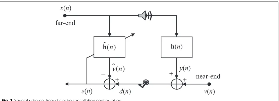
Let us consider the framework of a system identification problem (as shown in Fig. 1), like in AEC [1–9]. The far-end (or loudspeaker) signal,x(n), goes through the echo path, h(n), providing the echo signal, y(n), where n is the time index. This signal is added to the near-end sig-nal,v(n) (which can contain both the background noise and the near-end speech), resulting the microphone sig-nal,d(n). The adaptive filter, defined by the vectorh(n), aims to produce at its output an estimate of the echo,y(n), while the error signal,e(n), should contain an estimate of the near-end signal.
Summarizing, the main goal of this application is to model an unknown system using an adaptive filter, both driven by the same zero-mean input signal,x(n). These two systems are assumed to be finite impulse response (FIR) filters of length L, defined by the real-valued vectors:
h(n)=h0(n) h1(n) · · · hL−1(n)T, h(n)=h0(n)h1(n) · · ·hL−1(n)
T
,
Fig. 1General scheme. Acoustic echo cancellation configuration
d(n)=xT(n)h(n)+v(n) (1)
=y(n)+v(n), where
x(n)=x(n) x(n−1) · · · x(n−L+1)T
is a real-valued vector containing theLmost recent time samples of the input signal,x(n), andv(n)(i.e., the near-end signal) plays the role of the system noise (assumed to be quasi-stationary, zero mean, and independent ofx(n)) that corrupts the output of the unknown system.
Using the previous notation, we may define the a priori and a posteriori error signals as
e(n)=d(n)−xT(n)h(n−1)
=xT(n)
h(n)−h(n−1)
+v(n), (2) ε(n)=d(n)−xT(n)h(n)
=xT(n)h(n)−h(n)+v(n), (3)
where the vectorsh(n−1)andh(n)contain the adaptive filter coefficients at timen−1 andn, respectively. The update equation for NLMS-type algorithms is
h(n)=h(n−1)+μ(n)x(n)e(n), (4)
where μ(n) is a positive factor known as the step-size, which governs the stability, the convergence rate, and the misadjustment of the algorithm. A reasonable way to deriveμ(n), taking into account the stability conditions, is to cancel the a posteriori error signal [27]. Replacing (4) in (3) with the requirementε(n)=0, it results that
ε(n)=e(n)
1−μ(n)xT(n)x(n)
=0 (5)
and assuming thate(n)=0, we find
μ(n)= 1
xT(n)x(n). (6)
We should note that the above procedure makes sense in the absence of noise [i.e., v(n) = 0], where the con-dition ε(n) = 0 implies thatxT(n)
h(n)−h(n)
= 0. Finding the parameterμ(n)in the presence of noise will introduce noise inh(n), since the conditionε(n)=0 leads toxT(n)
h(n)−h(n)
= −v(n) = 0. In fact, we would
like to havexT(n)
h(n)−h(n)
= 0, which implies that ε(n)=v(n).
In practice, a positive constant α (with 0 < α < 2), known as the normalized step-size, multiplies (6) to achieve a proper compromise between the convergence rate and the misadjustment [10–12]; also, a positive con-stantδ, known as the regularization parameter, is added to the denominator of (6) in order to make the adaptive filter work well in the presence of noise. Consequently, the well-known update equation of the NLMS algorithm becomes
h(n)=h(n−1)+ αx(n)e(n)
xT(n)x(n)+δ. (7)
1.2.1 Performance analysis
Both the control parameters, i.e.,α andδ, highly influ-ence the overall performance of the NLMS algorithm. An insightful analysis of their influence was developed by Hänsler and Schmidt in [1]. To begin, let us define the a posteriori misalignment (also known as the system mismatch [1]) as
m(n)=h(n)−h(n). (8)
Assuming that the unknown system is time-invariant, i.e.,
h(n)=h(n−1), (9)
terms of the a posteriori misalignment. Consequently, it results
m(n)=m(n−1)− αx(n)e(n)
xT(n)x(n)+δ. (10)
Taking the2norm in (10), we obtain
m(n)22= m(n−1)22−2αm
Based on (2) and (9), the a priori error signal can be expressed as
e(n)=xT(n)m(n−1)+v(n), (12)
so that, using (12) in (11), it results
m(n)22= m(n−1)22
Next, taking mathematical expectation on both sides of (13) and removing the uncorrelated products (sincex(n) andv(n)are assumed to be independent and zero mean), we obtain is the variance of the input signal. For large values ofL(i.e., L1), it holds thatx(n)22≈Lσx2[1, 19]. Consequently,
so that, for a large value of L and a certain stationar-ity degree of the input signal, we can treat this term as
a deterministic quantity at this point [1]. Under these circumstances, (14) becomes a posteriori misalignment vector,m(n−1), are statistically independent, andx(n)is white. In this case,
E
Summarizing, (16) can be rewritten as
Em(n)22=Aα,δ,L,σx2Em(n−1)22
represent the so-calledcontractionandexpansion param-eters, respectively [1].
Clearly, the contraction parameter, Aα,δ,L,σx2, should be always smaller than 1, which is certainly ful-filled for 0< α <2 andδ≥0. The expansion parameter, Bα,δ,L,σ2
x
of the system noise). For example, taking the normalized step-size as the reference parameter and evaluating
∂Aα,δ,L,σx2
Neglecting the regularization constant (i.e.,δ ≈ 0), the fastest convergence mode is achieved forα≈1, which is a well-known result [1, 11, 12]. Also, the stability condition can be found by imposingA(α,δ,L,σx2)<1, which leads
Again, takingδ=0 in (23), the standard stability condi-tion of the NLMS algorithm results, i.e., 0< α <2. On the other hand, the lowest misadjustment (LM) is obtained when the term from (20) reaches its minimum. Also, tak-ing the normalized step-size as the reference parameter and evaluating
the lowest misadjustment mode requires
αLM=0, (25)
which is also a well-known result [1, 11, 12]; unfortunately, the filter is not updated in this case.
Summarizing, the convergence rate of the algorithm is not influenced by the level of the system noise, but the misadjustment increases when the system noise increases. More importantly, it can be noticed that the expansion term from (20) always increases when α increases; this concludes the fact that a higher value of the normalized step-size increases the misadjustment. Nevertheless, the ideal requirements of the algorithm are for both fast con-vergence and low misadjustment. It is clear that (22) and (25) “push” the normalized step-size in opposite direc-tions. This aspect represents the motivation behind the VSS approaches, i.e., the normalized step-size needs to be controlled in order to meet these conflicting require-ments. The regularization constant also influences the performance of the algorithm, but in a “milder” way. It can be noticed that the contraction term from (19) always decreases when the regularization constant increases, while the expansion term from (20) always increases when the regularization constant decreases.
1.2.2 Optimal choice of the control parameters
Motivated by these findings, Hänsler and Schmidt pro-posed in [1] (Chapter 13) an optimal choice for the control parameters of the NLMS algorithm. First, the
non-regularized version of the NLMS algorithm is consid-ered (also imposing that the normalized step-size is time dependent), with the update
h(n)=h(n−1)+ α(n)x(n)e(n)
x(n)22 . (26) Next, developing in (12), it results
xT(n)m(n−1)=e(n)−v(n)eu(n), (27)
whereeu(n)denotes the so-called undistorted error signal [1], i.e., the part of the error that is not affected by the system noise. Using this notation, (11) can be rewritten as
m(n)22= m(n−1)22−2α(n)eu(n)e(n)
A natural optimization criterion to follow in any sys-tem identification problem is the minimization of syssys-tem misalignment. Consequently, imposing the condition:
∂Em(n)22
and assuming that the normalized step-sizes at different time instants are uncorrelated, the optimal normalized step-size results as
For large values of L (i.e., L 1), the assumption
x(n)22 ≈ Lσx2is valid [1, 19]. Also, since the input sig-nal,x(n), and the system noise,v(n), are uncorrelated, the undistorted error signal,eu(n), is also uncorrelated with the system noise. Therefore, (31) simplifies to
αopt(n)= E
e2u(n)
Ee2(n). (32)
signal,eu(n), decreases and, consequently, the normalized step-size decreases, thus leading to low misadjustment.
Unfortunately, the undistorted error signal,eu(n), is not available in practice. In order to overcome this issue, sev-eral solutions were proposed in [1]. For example, assuming that the excitation,x(n), is white and considering that the input vector,x(n), and the a posteriori misalignment vec-tor, m(n− 1), are statistically independent, (32) can be developed based on (17) as
αopt(n)= E
Now the problem is reduced to the estimation of Em(n−1)22. A solution to estimate this term is based on the “delay and extrapolation” approach [1]. In other words, if an additional artificial delay is introduced into the unknown system, this delay is also modeled by the adaptive filter. Thus, utilizing the property of adaptive algorithms to spread the filter misalignment evenly over all coefficients, the known part of the (true) system mis-alignment vector can be extrapolated, thus resulting
m(n−1)22≈ L LD
LD−1
l=0
h2l(n), (34)
whereLDdenotes the number of coefficients correspond-ing to the artificial delay. However, this method may freeze the adaptation when the unknown system changes, which would require an additional system change detector [1].
The second control parameter of the NLMS algorithm is the regularization term,δ. Using a similar approach as before, the only-regularized version of the NLMS algo-rithm is considered (also imposing that the regularization parameter is time dependent), with the update
h(n)=h(n−1)+ x(n)e(n)
x(n)22+δ(n). (35)
In this case, (11) can be rewritten as
m(n)22= m(n−1)22−2 eu(n)e(n)
Following the same criterion, i.e., minimization of sys-tem misalignment, it can be imposed that the condition
∂Em(n)22
Under similar considerations and assumptions as in the case of αopt(n), (38) leads to the optimal regularization parameter, which can be further developed as
δopt(n)=
The denominator of (39) can be evaluated based on (34). Also, another important parameter to be found is the noise power,σ2
v. There are different methods for
esti-mating this parameter; for example, in echo cancellation, it can be estimated during silences of the near-end talker [19]. Also, other practical methods to estimateσ2
v in AEC
can be found in [28, 29] (which are briefly detailed in the end of Section 1.3). However, we should note that differ-ent other estimators can be used for the noise power; the analysis of their influence on the algorithms’ performance is beyond the scope of this paper.
Concluding, both control methods proposed by Hänsler and Schmidt in [1] [i.e.,αopt(n)andδopt(n)] are theoret-ically equivalent and represent valuable benchmarks in the field of VSS/VR-NLMS algorithms. However, in prac-tice, their implementations are usually different. In most cases, the control of the normalized step-size is preferred, mainly due to the limited dynamic range of its values; on the other hand, the regularization control usually requires an upper bound (to avoid overflow in case of very large values).
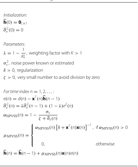
1.3 NPVSS-NLMS algorithm
Consequently, getting back to the discussion related to (2)–(6), the step-size parameter,μ(n)(which is determin-istic in nature), can be found by imposing the condition [19]
Eε2(n)=σv2. (40)
Following this requirement, we rewrite (5) as
ε(n)=e(n)1−μ(n)xT(n)x(n)=v(n). (41)
Squaring the previous equation, then taking mathemat-ical expectation on both sides, and using the approxima-tionxT(n)x(n) ≈ LEx2(n) = Lσx2 (which is valid for Thus, developing (42), we obtain the quadratic equation
μ2(n)− 2
for which the obvious solution is (also using Lσx2 ≈ xT(n)x(n))
is the variable normalized step-size. Therefore, the update of the non-parametric variable step-size NLMS (NPVSS-NLMS) algorithm [19] is
h(n)=h(n−1)+μNPVSS(n)x(n)e(n). (46)
Let us examine the behavior of the algorithm in terms of its normalized step-size. Looking at (44), it is obvious that before the algorithm converges,σe(n) is large compared
toσvand, consequently,αNPVSS(n) ≈ 1. When the
algo-rithm has converged to the true solution,σe(n) ≈σvand αNPVSS(n)≈0. This is the desired behavior for the adap-tive algorithm, leading to both fast convergence and low misadjustment.
We can compare (45) to the optimal step-size parameter from (32), which results in
αopt(n)=αNPVSS(n) between 1 and 2, but the two variable step-sizes have the same effect for good convergence and low misadjustment. In order to analyze the convergence of the misalign-ment for the NPVSS-NLMS algorithm, we suppose that the system is stationary (as in (9)). Using the a posteriori
misalignment vector defined in (8), the update equation of the algorithm (46) can be rewritten in terms of the misalignment as
m(n)=m(n−1)−μNPVSS(n)x(n)e(n). (48)
Taking thel2norm in (48), then mathematical expecta-tion on both sides, and assuming that
E
The previous expression proves that the length of the misalignment vector for the NPVSS-NLMS algorithm is non-increasing, which implies that
lim
n→∞σ 2
e(n)=σv2. (51)
It should be noticed that the previous relation does not imply that Em(∞)22 = 0. However, under the independence assumption, we can show the equivalence. Indeed, from (12), it can be shown that
Ee2(n)=σv2+tr [RK(n−1)] (52)
ifx(n)are independent (i.e., the white input assumption), where tr(·) is the trace of a matrix,R = Ex(n)xT(n), andK(n−1)=Em(n−1)mT(n−1). Taking (51) into account, (52) becomes
tr [RK(∞)]=0. (53)
Assuming that R > 0 (i.e., R is a positive definite matrix), it results thatK(∞)=0and, consequently,
Em(∞)22=0. (54)
Finally, some practical considerations have to be stated. First, in order that the algorithm behaves properly, a regu-larization constant,δ, should be added to the denominator ofμNPVSS(n). A second consideration is related to the esti-mation of the parameterσe(n). In practice, the power of
the error signal is estimated as follows:
σ2
e(n)=λσe2(n−1)+(1−λ)e2(n), (55)
whereλis a weighting factor. Its value is chosen asλ = 1− 1/(KL), where K > 1. The initial value for (55) is
σ2
e(0) = 0. Theoretically, it is clear that σe2(n) ≥ σv2,
which implies thatμNPVSS(n)≥0. Nevertheless, the esti-mation from (55) could result in a lower magnitude than the noise power estimate, which would makeμNPVSS(n) negative. In this situation, the problem is solved by setting μNPVSS(n)=0.
Table 1NPVSS-NLMS algorithm
KL, weighting factor withK>1 σ2
v, noise power known or estimated δ >0, regularization
ζ >0, very small number to avoid division by zero
For time index n=1, 2,. . .:
of the NPVSS-NLMS algorithm is the power estimate of the system noise. In the case of AEC, this system noise is represented by the near-end signal. Nevertheless, the esti-mation of the near-end signal power is not always straight-forward in real-world AEC applications. Some practical solutions to this problem can be found in [28, 29].
For example, it was demonstrated in [28] that the power estimate of the near-end signal can be evaluated as
σ2
where the variance ofe(n)is estimated based on (55) and the other terms are evaluated in a similar manner, i.e.,
σ2
x(n)=λσx2(n−1)+(1−λ)x2(n), (57) rex(n)=λrex(n−1)+(1−λ)x(n)e(n). (58)
A more practical solution was proposed in [29]. It is known that the desired signal of the adaptive filter is expressed asd(n)=y(n)+v(n). Since the echo signal and the near-end signal can be considered uncorrelated, the previous relation can be rewritten in terms of variances as
Ed2(n)=Ey2(n)+Ev2(n). (59)
Assuming that the adaptive filter has converged to a certain degree, we can use the approximation
Ey2(n)≈Ey2(n). (60)
Consequently, using power estimates, we may compute
σ2
v(n)=σd2(n)−σy2(n), (61)
whereσd2(n) andσy2(n)are the power estimates of d(n) andy(n), respectively. These parameters can be recur-sively evaluated similar to (55), i.e.,
σ2
d(n)=λσd2(n−1)+(1−λ)d2(n), (62) σ2
y(n)=λσy2(n−1)+(1−λ)y2(n). (63)
The absolute values in (61) prevent any minor devia-tions (due to the use of power estimates) from the true values, which can make the normalized step-size negative or complex.
When only the background noise is present, an estimate of its power is obtained using the right-hand term in (61). This expression holds even if the level of the background noise changes, so that there is no need for the estimation of this parameter during silences of the near-end talker. In case of double-talk, when the near-end speech is also present (assuming that it is uncorrelated with the back-ground noise), the right-hand term in (61) still provides a power estimate of the near-end signal. Most importantly, this term depends only on the signals that are available within the AEC application, i.e., the microphone signal, d(n), and the output of the adaptive filter,y(n). Moreover, as it was demonstrated in [29], the estimation from (61) is also suitable for the under-modeling case, i.e., when the length ofh(n) is smaller than the length ofh(n), so that an under-modeling noise appears (i.e., the residual echo caused by the part of the echo path that is not modeled by the adaptive filter; it can be interpreted as an additional noise that corrupts the near-end signal).
The main drawback of (61) is due to the approximation in (60). This assumption will be biased in the initial con-vergence phase or when there is a change of the echo path. Concerning the first problem, we can use a regular NLMS algorithm in the first steps (e.g., in the firstLiterations).
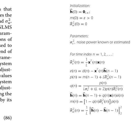
1.4 JO-NLMS algorithm
assuming thath(n)is a zero-mean random vector, which follows a simplified first-order Markov model, i.e.,
h(n)=h(n−1)+w(n), (64)
where w(n) is a zero-mean white Gaussian noise signal vector, which is uncorrelated withh(n−1). The correla-tion matrix ofw(n)is assumed to beRw=σw2IL, whereIL
is theL×Lidentity matrix. The variance,σw2, captures the uncertainties inh(n). Equations (1) and (64) define now a state variable model, similar to Kalman filtering setup.
1.4.1 Convergence analysis
In the context of the previously defined model, let us con-sider the update of the NLMS algorithm from (7). Next, developing (7) in terms of the a posteriori misalignment from (8), also taking (64) into account, we obtain
m(n)=m(n−1)+w(n)− αx(n)e(n)
This term contains both the control parameters, i.e.,α andδ, and also the statistical information on the input signal. However, for a large value ofLand a certain sta-tionarity degree of the input signal, we can treat this term as a deterministic quantity [1].
Under these circumstances, taking the2norm in (65), then mathematical expectation on both sides (also using (66)), and removing the uncorrelated products, we obtain
Em(n)22=Em(n−1)22
In order to further process (67), let us focus on its last three cross-correlation terms. Based on (1), (8), and (64), the a priori error signal from (2) can be rewritten as
e(n)=xT(n)m(n−1)+xT(n)w(n)+v(n). (68)
Therefore, taking (68) into account within the first cross-correlation term from (67) (also removing the uncorrelated products), it results in
EmT(n−1)x(n)e(n)≈EmT(n−1)x(n)xT(n)m(n−1)
Next, the following assumptions can be considered: (i) the a posteriori misalignment at time indexn−1 is uncor-related with the input vector at time index n and (ii) the correlation matrix of the input is close to a diagonal one, i.e.,Ex(n)xT(n) ≈ σ2
xIL (this is a fairly restrictive
assumption, however, it has been widely used to simplify the analysis [16]). Consequently, (69) becomes
E
The second cross-correlation term from (67) can be also developed based on (68). Taking into account that the cor-relation matrix of w(n) is assumed to be diagonal and removing the uncorrelated products, it results in
EwT(n)x(n)e(n)=EwT(n)x(n)xT(n)w(n)
The last expectation term from (67) can be also expressed taking (68) into account. Using a similar approach, it results in
Gaussian moment factoring theorem [32] (also known as the Isserlis’ theorem) and results in
E
Therefore, using the result from (73), (72) becomes
Ee2(n)xT(n)x(n)
Having all these terms, we can introduce (70), (71), and (74) in (67), also denotingm(n)=Em(n)22, to obtain
The result from (75) illustrates a “separation” between the convergence and misadjustment components, simi-lar to (18)–(20) from Section 1.2. Therefore, the term
Aα,δ,L,σx2influences the convergence rate of the algo-rithm. As expected, it depends on the normalized step-size value, the regularization constant, the filter length, and the input signal power. It is interesting to notice that it does not depend on the system noise power, σv2, or the uncertainties, σw2; in other words, the convergence rate should not be influenced by these two terms. In fact, the term from (76) is very similar to the contraction
parameter, Aα,δ,L,σx2, from (19). Similarly, it can be noticed that the fastest convergence mode is obtained when the function from (76) reaches its minimum. Taking the normalized step-size as the reference parameter, we obtain
αFC= δ+Lσx2 (L+2)σ2
x
, (78)
which is similar to the result obtained in (22). For exam-ple, neglecting the regularization constant (i.e.,δ≈0) and
assuming that L 2, the fastest convergence mode is
achieved forα ≈1, which is the same conclusion related to (22). Also, similar to (23), the stability condition can be found by imposingA(α,δ,L,σ2 dard stability condition of the NLMS algorithm results, i.e., 0< α <2.
The termB(α,δ,L,σ2
x,σv2,σw2)influences the
misadjust-ment of the algorithm and it depends on bothσ2 v andσw2
(clearly, the misadjustment increases when these two fac-tors increase). As we can notice, it is very similar to the expansion parameter,Bα,δ,L,σx2, from (20), except the fact that the term from (77) includes now the contribu-tions ofσv2andσw2. However, the lowest misadjustment is obtained in a similar way, i.e., when the function from (77) reaches its minimum. Thus, taking the normalized step-size as the reference parameter, the lowest misadjustment is achieved for
In order to compare this result with (25), let us assume that the system is time-invariant, i.e., σw2 ≈ 0. Conse-quently, (80) leads toα≈0 (i.e., the lowest misadjustment is obtained for a normalized step-size close to zero), which is the same result obtained in (25).
1.4.2 Derivation of the algorithm
Thus, following (75) and considering that the two important parameters are time dependent, it can be imposed
∂m(n)
∂α(n) =0, (81)
∂m(n)
∂δ(n) =0. (82)
After straightforward computations, both equations lead to the same result, i.e.,
α(n)
which suggests a joint optimization process. With a proper estimation of its parameters (as will be discussed in the end of this section), the term from the right-hand side of (83) acts like a variable step-size. At this point, we can introduce (83) in (7), thus obtaining
h(n)=h(n−1)+ (84). Using (83) in (75), followed by several straightfor-ward computations, it results in
m(n)= 1− σ
Consequently, the resulting JO-NLMS algorithm is defined by the relations (2), (84), and (85).
Finally, there are some practical considerations that should be outlined. The JO-NLMS algorithm requires the estimation of three main parameters, i.e.,σx2,σv2, andσw2. The first one can be easily evaluated as in the NLMS algorithm, i.e.,σx2(n) = L1xT(n)x(n). The second param-eter (i.e., σv2) appears in many VSS and VR versions of the NLMS algorithm. Different methods can be used to estimate it, e.g., [19, 28, 29], as mentioned at the end of Sections 1.2 and 1.3. Maybe the most important parame-ter to be found isσw2. Small values ofσw2(i.e., the system is assumed to be time-invariant) imply a good misadjust-ment but a poor tracking; on the other hand, large values ofσ2
w(i.e., assuming that the uncertainties in the system
are high) imply a good tracking but a high misadjust-ment. In practice, we propose to estimateσw2by taking the 2norm on both sides of (64) and replacing h(n)by its ues in the beginning of adaptation (or when there is an abrupt change of the system), thus providing fast conver-gence and tracking. On the other hand, when the algo-rithm starts to converge, the value ofσ2
w(n)reduces, which
leads to low misadjustment. In this way, the algorithm achieves a proper compromise between the performance criteria. In finite precision implementations, in order to avoid any risk of freezing in (86), it is recommended to set a lower bound forσw2(n)(e.g., the smallest positive number available).
The JO-NLMS algorithm is summarized in Table 2, in such a way that its implementation is facilitated. This algo-rithm is similar to the simplified Kalman filter presented in [31]. However, contrary to this one (which was obtained as an approximation of the general Kalman filter), the JO-NLMS algorithm was derived in a different manner following a specific optimization criterion. In fact, this is an alternative way to obtain the same results as with the Kalman filter.
1.5 Simulation results
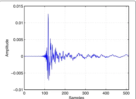
Simulations were performed in an AEC configuration, as shown in Fig. 1. The measured acoustic impulse response was truncated to 512 coefficients (Fig. 2), and the same length was used for the adaptive filter, i.e.,L = 512; the sampling rate is 8 kHz. We should note that in many real-world AEC scenarios, the adaptive filter works most likely in an under-modeling situation, i.e., its length is
Table 2JO-NLMS algorithm
v, noise power known or estimated
Fig. 2Echo path. Acoustic impulse response used in simulations
smaller than the length of the acoustic impulse response. Hence, the residual echo caused by the part of the sys-tem that cannot be modeled acts like an additional noise (that corrupts the near-end signal) and disturbs the over-all performance. However, for experimental purposes, we set the same length for both the unknown system (i.e., the acoustic echo path) and the adaptive filter.
The input signal,x(n), is either a white Gaussian noise, an AR(1) process generated by filtering a white Gaussian noise through a first-order system 1/1−0.8z−1 or a speech sequence. An independent white Gaussian noise v(n) is added to the echo signaly(n), with SNR = 20 dB (except in the last experiment where the SNR is variable and the near-end speech is also present). In most of the experiments (except in the last one), we assume thatσ2
v is
known; in practice, this variance can be estimated like in [19, 28, 29] (as presented in the end of Section 1.3). The tracking capability of the algorithm is an important issue in AEC, where the acoustic impulse response may rapidly change at any time during the connection. Consequently, an echo path change scenario is simulated in most of the experiments, by shifting the impulse response to the right by 12 samples, in the middle of the experiment. The mea-sure of performance is the normalized misalignment (in dB), defined as
m(n)=20 log10h(n)−h(n)
2/h(n)2
. (87)
In the first set of experiments, we evaluate the per-formance of the optimal control parameters proposed by Hänsler and Schmidt in [1] (also summarized in Section 1.2), in order to set the benchmark for further comparisons. In this context, we consider the ideal esti-mation of these parameters [i.e.,αopt(n)andδopt(n)from Section 1.2], assuming that the undistorted error signal
eu(n) from (27) is available and its power, Ee2u(n) = σ2
eu(n), can be evaluated similar to (55), i.e.,
σ2
eu(n)=λσ 2
eu(n−1)+(1−λ)e 2 u(n) =λσ2
eu(n−1)+(1−λ)[e(n)−v(n)]
2, (88)
whereλis a weighting factor [λ=1−1/(KL), withK>1]. Of course, in practice, the near-end signalv(n)is not avail-able; however, for comparison purpose, we consider that it is available in (88).
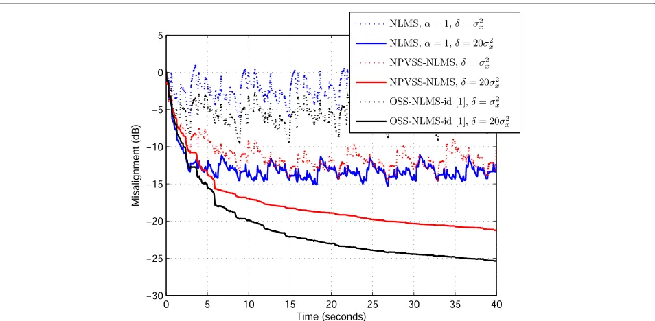
In the first simulation, we evaluate the performance of the NLMS algorithm using αopt(n) and δopt(n), respec-tively. Since the estimation from (88) is used for both these parameters, we deal with the ideal behavior of the algo-rithms. Consequently, we will refer to these algorithms as the ideal optimal step-size NLMS (OSS-NLMS-id) and the ideal optimal regularized NLMS (OR-NLMS-id), respectively. In Fig. 3, these ideal benchmarks are compared to the NLMS algorithm using different con-stant values of the normalized step-size, α, and reg-ularization parameter, δ; the input signal is a white Gaussian noise. First, it can be noticed that the perfor-mance of the regular NLMS algorithm can be controlled
in terms of both parameters, α and δ, either by
set-ting the fastest convergence mode (i.e., α = 1) and
adjusting the value of δ, or by neglecting the regular-ization constant (i.e., δ = 0) and tuning the value of
α. On the other hand, in case of the optimal control
parameters, the OSS-NLMS-id and OR-NLMS-id algo-rithms achieve both fast convergence/tracking and low misalignment, outperforming the NLMS algorithms that use constant values for α and δ. Besides, it should be noted that the OSS-NLMS-id and OR-NLMS-id algo-rithms are equivalent in terms of their performance (their misalignment curves are overlapped), which jus-tifies the findings from Section 1.2. For this experi-ment, the evolution of αopt(n)andδopt(n)is depicted in Fig. 4, also supporting the expected behavior of these parameters.
Fig. 3Performance of the optimal algorithms for white Gaussian input. Misalignment of the NLMS (for different values ofαandδ), OSS-NLMS-id, and OR-NLMS-id algorithms. The input signal is white Gaussian, echo path changes at time 10 s,L=512, and SNR = 20 dB
difficult to control the adaptation in terms of the regu-larization term, since its values are increasing and could lead to overflows. Usually, an upper bound on the reg-ularization parameter could be imposed, but this would introduce an extra tuning parameter in the algorithm.
Due to these aspects, only the OSS-NLMS-id algorithm will be considered as a benchmark in the following experiments.
Nevertheless, the OSS-NLMS-id algorithm still requires a constant regularization parameter, especially in case of
Fig. 5Performance of the optimal algorithms for AR(1) input. Misalignment of the NLMS (for different values ofαandδ), OSS-NLMS-id, and OR-NLMS-id algorithms. The input signal is an AR(1) process, echo path changes at time 40 s,L=512, and SNR = 20 dB
non-stationary inputs like speech. This is also the case of the NPVSS-NLMS algorithm presented in Section 1.3. While in the previous experiments, this regularization constant was neglected (due to the stationary nature of the input signals), and the next simulation shows the
importance of this parameter in practice. For this pur-pose, in Fig. 7, a speech sequence is considered at the far-end. The NLMS, NPVSS-NLMS, and OSS-NLMS-id algorithms are compared when using two different val-ues of the regularization constant, i.e.,δ = σx2andδ =
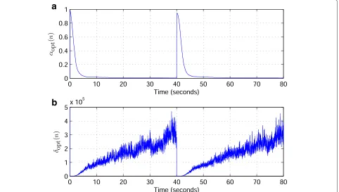
Fig. 6Optimal control parameters for AR(1) input. Evolution of the optimal control parameters:aαopt(n)of the OSS-NLMS-id algorithm andb
Fig. 7Regularization influence on the algorithms’ performance. Misalignment of the NLMS (withα=1), NPVSS-NLMS, and OSS-NLMS-id algorithms for different values ofδ. The input signal is speech,L=512, and SNR = 20 dB
20σ2
x. As expected, the small regularization is not
suit-able in this case, leading to large misalignment. On the other hand, the rule of thumbδ = 20σx2 (used in many echo cancellation scenarios [6–8]) is more appropriate here. Thus, the regularization parameter is a must in this case. In fact, the regularization parameter is required in all ill-posed and ill-conditioned problems such as in AEC; some insights for choosing this parameter in practice can be found in [14]. However, in all the following
experi-ments, we will consider a constant regularization δ =
20σx2 for the NLMS, NPVSS-NLMS, and OSS-NLMS-id
algorithms. As shown in [14], the regularization parame-ter of the NLMS algorithm is related to the value of SNR and the filter’s lengthL. For our experimental setup, i.e.,
L = 512 and SNR = 20 dB, the value δ = 20σ2
x fits
well. However, this value should be increased for larger values ofLor lower SNRs [14]. To conclude this exper-iment, the influence of the regularization parameter can be also noticed in Fig. 8, where the control parameters of the NPVSS-NLMS and OSS-NLMS-id algorithms are depicted, i.e.,αNPVSS(n)andαopt(n), respectively. Clearly, their behavior is strongly biased in case of the small regularization parameter, while they perform similarly in case of a proper regularization.
Next, the JO-NLMS algorithm (presented in
Section 1.4) is also involved in the rest of experiments. As compared to its counterparts, this algorithm does not require an explicit regularization term. Its global step-size from (83) resulted based on the joint-optimization on both the normalized step-size and regularization
parameter. In Figs. 9 and 10, the NLMS algorithm (for
different values of α) is compared with the
NPVSS-NLMS, JO-NLMS, and OSS-NLMS-id algorithms,
when the far-end signal is an AR(1) process or a speech sequence, respectively. According to these results, it can be noticed that the NLMS algorithm is clearly outperformed by the other algorithms, in terms of con-vergence rate, tracking, and misalignment. Also, the NPVSS-NLMS and JO-NLMS algorithms perform in a similar manner (with a slight advantage for the JO-NLMS algorithm); besides, they are close to the performance of the OSS-NLMS-id algorithm, which represents the ideal benchmark.
Fig. 8Regularization influence on the control parameters. Evolution of the normalized step-sizes of the NPVSS-NLMS algorithm [αNPVSS(n)] and OSS-NLMS-id algorithm [αopt(n)] for different values ofδ:aδ=σx2andbδ=20σx2. Other conditions are the same as in Fig. 7
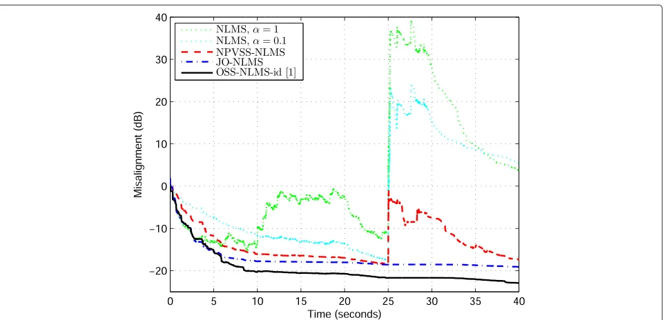
Fig. 10Performance of the algorithms for speech input. Misalignment of the NLMS (for different values ofα), NPVSS-NLMS, JO-NLMS, and OSS-NLMS-id algorithms. The input signal is speech; echo path changes at time 20 s,L=512, and SNR = 20 dB
simulated, by decreasing the SNR from 20 to 10 dB between times 10 and 20 s; second, the near-end speech appears between times 25 and 30 s (i.e., double-talk case), without using any DTD. The results from Fig. 11 indi-cate that the NLMS algorithm fails in this case, especially during double-talk. The NPVSS-NLMS and JO-NLMS
algorithms show good robustness features in both situ-ations (with an advantage for the JO-NLMS algorithm during double-talk). In terms of robustness, the JO-NLMS algorithm performs similar to the ideal case repre-sented by the OSS-NLMS-id algorithm. Finally, it should be noted that both the NPVSS-NLMS and JO-NLMS
Fig. 11Performance of the algorithms during near-end variations. Misalignment of the NLMS (for different values ofα), NPVSS-NLMS, JO-NLMS, and OSS-NLMS-id algorithms. The NPVSS-NLMS and JO-NLMS algorithms use the estimatedσ2
v(n)from (61). The input signal is speech,L=512, and
algorithms do not require any additional features to control their behavior, thus being reliable candidates for AEC applications.
2 Conclusions
In this paper, we have presented several NLMS-based algorithms suitable for AEC applications. These algo-rithms are based on different control strategies for adjust-ing their main parameters, i.e., the normalized step-size and regularization term, in order to achieve a proper compromise between the performance criteria (i.e., fast convergence/tracking and low misadjustment). The main motivation behind this approach was the reference work of Hänsler and Schmidt from [1]. Following their ideas, we presented here two related solutions, i.e., the NPVSS-NLMS and JO-NPVSS-NLMS algorithms. The first one (originally proposed in [19]) represents a simple and efficient method to control the normalized step-size. Due to its non-parametric nature, it is a reliable choice in many practical applications. The second one is developed in the con-text of a state-variable model and follows an optimization criterion based on the minimization of the system mis-alignment. It is also a non-parametric algorithm, which does not require any additional control features (e.g., sys-tem change detector, stability thresholds, etc.). It also gives good robustness against double-talk, which is one of the most challenging situation in AEC. Consequently, it could be an appealing candidate for real-world applications.
There are several perspectives that could follow the ideas presented in this paper. First, the extension to the affine projection algorithm represents a straightforward approach. Second, it would be highly interesting to further develop these solutions in the context of proportionate-type algorithms, which are also attractive choices for sparse system identification.
Concluding, despite the fact that the NLMS algorithm was the workhorse in AEC and also in many other applica-tions, it is still highly studied and very often represents the algorithm of choice in practice. Therefore, let us end this paper with a neat remark of Hänsler and Schmidt from [4], which fits best in this context: “The NLMS algorithm has often been declared to be dead. According to a popular saying, this is an infallible sign of a very long life.”
Competing interests
The authors declare that they have no competing interests.
Acknowledgements
This work was supported by the UEFISCDI Romania under Grant PN-II-RU-TE-2014-4-1880.
Author details
1Department of Telecommunications, University Politehnica of Bucharest, 1-3 Iuliu Maniu Blvd., 061071 Bucharest, Romania.2INRS-EMT, University of Quebec, 800 de la Gauchetière Ouest, QC H5A 1K6 Montreal, Canada. 3Department of Electrical and Computer Engineering, Missouri University of
Science and Technology, 301 W. 16th St., 65409-0040 Rolla, USA.
Received: 30 June 2015 Accepted: 6 November 2015
References
1. E Hänsler, G Schmidt,Acoustic Echo and Noise Control—A Practical Approach. (Wiley, Hoboken, NJ, 2004)
2. E Hänsler, The hands-free telephone problem—an annotated bibliography. Signal Process.27(3), 259–271 (1992)
3. E Hänsler, G Schmidt, Hands-free telephones—joint control of echo cancellation and post filtering. Signal Process.80(11), 2295–2305 (2000) 4. E Hänsler, G Schmidt, inLeast-Mean-Square Adaptive Filters, ed. by
S Haykin, B Widrow. Control of LMS-type adaptive filters (Wiley New York, NY, 2003), pp. 175–240
5. E Hänsler, inEncyclopedia of Telecommunications, ed. by J Proakis. Acoustic echo cancellation (Wiley New York, NY, 2003), pp. 1–15 6. SL Gay, J Benesty (eds.),Acoustic Signal Processing for Telecommunication
(Kluwer Academic Publisher, Boston, MA, 2000)
7. J Benesty, T Gänsler, DR Morgan, MM Sondhi, SL Gay,Advances in Network and Acoustic Echo Cancellation. (Springer-Verlag, Berlin, Germany, 2001) 8. J Benesty, Y Huang (eds.),Adaptive Signal Processing—Applications to
Real-World Problems(Springer-Verlag, Berlin, Germany, 2003)
9. G Enzner, H Buchner, A Favrot, F Kuech, inAcademic Press, Library in Signal Processing, ed. by R Chellappa, S Theodoridis. Acoustic echo control, vol. 4 (Academic Press Chennai, 2014), pp. 807–877
10. B Widrow, SD Stearns,Adaptive Signal Processing. (Prentice Hall, Englewood Cliffs, NJ, 1985)
11. S Haykin,Adaptive Filter Theory, 4th edn. (Upper Saddle River, NJ, Prentice-Hall, 2002)
12. AH Sayed,Adaptive Filters. (Wiley, New York, NY, 2008)
13. C Breining, P Dreiseitel, E Hänsler, A Mader, B Nitsch, H Puder, T Schertler, G Schmidt, J Tilp, Acoustic echo control—an application of very-high-order adaptive filters. IEEE Signal Processing Mag.16(4), 42–69 (1999) 14. J Benesty, C Paleologu, S Ciochin˘a, On regularization in adaptive filtering.
IEEE Trans. Audio, Speech, Language Processing.19(6), 1734–1742 (2011) 15. A Mader, H Puder, GU Schmidt, Step-size control for acoustic echo
cancellation filters—an overview. Signal Process.80(9), 1697–1719 (2000) 16. AI Sulyman, A Zerguine, Convergence and steady-state analysis of a
variable step-size NLMS algorithm. Signal Process.83(6), 1255–1273 (2003) 17. H-C Shin, AH Sayed, W-J Song, Variable step-size NLMS and affine
projection algorithms. IEEE Signal Processing Lett.11(2), 132–135 (2004) 18. DP Mandic, A generalized normalized gradient descent algorithm. IEEE
Signal Processing Lett.11(2), 115–118 (2004)
19. J Benesty, H Rey, L Rey Vega, S Tressens, A nonparametric VSS-NLMS algorithm. IEEE Signal Processing Lett.13(10), 581–584 (2006) 20. Y-S Choi, H-C Shin, W-J Song, Robust regularization for normalized LMS
algorithms. IEEE Trans. Circuits and Systems II: Express Briefs.53(8), 627–631 (2006)
21. H Rey, L Rey Vega, S Tressens, J Benesty, Variable explicit regularization in affine projection algorithm: robustness issues and optimal choice. IEEE Trans. Signal Process.55(5), 2096–2108 (2007)
22. P Park, M Chang, N Kong, Scheduled-stepsize NLMS algorithm. IEEE Signal Processing Lett.16(12), 1055–1058 (2009)
23. H-C Huang, J Lee, A new variable step-size NLMS algorithm and its performance analysis. IEEE Trans. Signal Process.60(4), 2055–2060 (2012) 24. H-C Huang, J Lee, inProc. IEEE Asilomar. A variable regularization control
method for NLMS algorithm (Pacific Grove CA, 2012), pp. 396–400 25. I Song, P Park, A normalized least-mean-square algorithm based on
variable-step-size recursion with innovative input data. IEEE Signal Processing Lett.19(12), 817–820 (2012)
26. S Ciochin˘a, C Paleologu, J Benesty, An optimized NLMS algorithm for system identification. Signal Process.118(1), 115–121 (2016) 27. DR Morgan, SG Kratzer, On a class of computationally efficient, rapidly
converging, generalized NLMS algorithms. IEEE Signal Processing Lett. 3(8), 245–247 (1996)
28. MA Iqbal, SL Grant, inProc. IEEE International Conference on Acoustics, Speech and Signal Processing (ICASSP). Novel variable step size NLMS algorithms for echo cancellation (Las Vegas, NV, 2008), pp. 241–244 29. C Paleologu, S Ciochin˘a, J Benesty, Variable step-size NLMS algorithm for
30. G Enzner, P Vary, Frequency-domain adaptive Kalman filter for acoustic echo control in hands-free telephones. Signal Process.86(6), 1140–1156 (2006)
31. C Paleologu, J Benesty, S Ciochin˘a, Study of the general Kalman filter for echo cancellation. IEEE Trans. Audio, Speech, Language Processing.21(8), 1539–1549 (2013)
32. L Isserlis, On a formula for the product-moment coefficient of any order of a normal frequency distribution in any number of variables. Biometrika. 12(1/2), 134–139 (1918)
Submit your manuscript to a
journal and benefi t from:
7Convenient online submission
7Rigorous peer review
7Immediate publication on acceptance
7Open access: articles freely available online
7High visibility within the fi eld
7Retaining the copyright to your article

![Fig. 8 Regularization influence on the control parameters. Evolution of the normalized step-sizes of the NPVSS-NLMS algorithm [αNPVSS(n)] andOSS-NLMS-id algorithm [αopt(n)] for different values of δ: a δ = σ 2x and b δ = 20σ 2x](https://thumb-us.123doks.com/thumbv2/123dok_us/890762.1107167/16.595.60.538.451.698/regularization-influence-parameters-evolution-normalized-algorithm-algorithm-different.webp)