Training Methods for Image Noise Level
Estimation on Wavelet Components
A. De Stefano
Institute of Sound and Vibration Research, University of Southampton, Highfield, Hants SO17 1BJ, UK Email:[email protected]
P. R. White
Institute of Sound and Vibration Research, University of Southampton, Highfield, Hants SO17 1BJ, UK Email:[email protected]
W. B. Collis
The Foundry, 35-36 Great Marlborough Street, London W1F 7JE, UK Email:[email protected]
Received 25 July 2003; Revised 14 January 2004
The estimation of the standard deviation of noise contaminating an image is a fundamental step in wavelet-based noise reduction techniques. The method widely used is based on the mean absolute deviation (MAD). This model-based method assumes spe-cific characteristics of the noise-contaminated image component. Three novel and alternative methods for estimating the noise standard deviation are proposed in this work and compared with the MAD method. Two of these methods rely on a preliminary training stage in order to extract parameters which are then used in the application stage. The sets used for training and testing, 13 and 5 images, respectively, are fully disjoint. The third method assumes specific statistical distributions for image and noise components. Results showed the prevalence of the training-based methods for the images and the range of noise levels considered.
Keywords and phrases:noise estimation, training methods, wavelet transform, image processing.
1. INTRODUCTION
Noise reduction plays a fundamental role in image pro-cessing, and wavelet analysis has been demonstrated to be a powerful method for performing image noise reduction [1,2,3,4,5,6,7,8,9,10,11,12]. The procedure for noise reduction is applied on the wavelet coefficients achieved us-ing the wavelet decomposition and representus-ing the image at different scales. After noise reduction, the image is recon-structed using the inverse wavelet transform. Decomposi-tion and reconstrucDecomposi-tion are accomplished using two banks of filters constrained by a perfect reconstruction condition [3,13]. The structure of these filter banks is characterised by the frequency responses of two filters and by the pres-ence or abspres-ence of sub/up-sampling, generating, respectively, decimated or undecimated wavelet transforms. Undecimated wavelet transforms have been considered for image noise re-duction [3,4,5,6,10,11,12] as well as the decimated trans-forms [1,2,6,7,8,9].
Whilst alternative techniques have been proposed [14,15, 16,17,18], the technique most widely used to reduce the
highest resolution [1,2,6,7]. Nevertheless, in our literature research we did not find alternative methods addressed to this problem.
In this paper, we include an investigation of the problem of estimating the variance of the noise contaminating an im-age and we compare three novel algorithms, two of which based on training over a set of test images, with the MAD technique.
The training process extracts a number of parameters us-ing a set of noise-contaminated images generated by synthet-ically combining noise-free images with realisations of the noise process with a given level (standard deviation). During the application of the algorithm, only a noisy image is avail-able for analysis, from which the level of the contaminating noise is estimated employing the parameters extracted dur-ing the traindur-ing.
In Section 2, we present the three new techniques for noise level estimation over the wavelet components. The re-sults are described and commented upon in Section 3, and conclusions are drawn inSection 4.
2. NOISE LEVEL ESTIMATION
The most widely used method for estimating the variance of the noise on a wavelet component is the mean absolute deviation (MAD). This scheme tends to overestimate the noise standard deviation in applications where the SNR in the wavelet components is high, leading to unnecessary dis-tortion of the image. The tendency for MAD to overestimate the noise level is due to the fact that it assumes that the image contribution in the band of interest can be neglected. How-ever, the fact that MAD is based on absolute deviations makes it more robust to outliers (arising through image contribu-tions in the band) than, say, direct estimate of the standard deviation.
This section presents three alternative methods for esti-mating the standard deviation of the noise from a noisy im-age. These methods are based on the assumption that the noise is Gaussian and additive. The methods can be applied to any of the wavelet components of the image. However, their performance degrades when the signal-to-noise ratio (SNR) in the component increases, so in practice one usu-ally finds that the noise variance is most accurately estimated on the smallest scale (highest frequency) component where, in most cases, the SNR is the lowest. If one is willing to make the assumption of spatially white noise, then knowledge of the noise variance at the smallest scale allows the one to infer the noise variance at all other scales.
2.1. Model-based estimation of the noise variance
One method of estimating the noise variance is to assume a model for both the noise and image components and to fit the data to this model. One model, consistent with the use of a soft thresholding scheme, is to assume that the noise is additive and Gaussian and the image has a Laplacian distri-bution. If the Laplacian distribution has zero mean and stan-dard deviationσu, then its probability distribution function
(pdf) is
pim(x)= 1
σu√2e
−(√2/σu)|x|. (1)
The pdf of the image plus Gaussian noise (standard deviation
σv) is [3]
where erfc(x) is the complementary error function. The problem is then to estimate the parametersσuandσvfrom the observed pixel values. An optimal method to achieve this is to employ the method of maximum likelihood (ML). In this problem, ML leads to a solution with no closed analytic form and one is faced with an optimisation task. The absence of a sufficient statistic for this problem makes the computa-tion of the ML solucomputa-tion burdensome. At every iteracomputa-tion of the optimisation, one is required to evaluate (2) for every pixel in the image. In an off-line environment, this load may not be too onerous, but for real-time implementation presents a significant challenge.
An efficient, but suboptimal, alternative is to employ the method of matching moments [25,26]. The technique pre-sented here is based on the 2nd and 4th moments of the data. Assuming a Laplacian model for the image and a Gaussian noise distribution, then the 2nd and 4th moments of the im-age plus noise are given by
Ex2=m
2=σu2+σv2, Ex4=m
4=6σu4+ 3σv4+ 6σu2σv2.
(3)
The moment matching method utilizes estimates of the mo-ments,m2andm4obtained directly from the data using
mk=N1 m,nx
(m,n)k. (4)
Replacing the theoretical momentsmk, by their estimatesmk, and solving (3) for the unknown noise variance, one obtains
σv2=m
The above has a pleasant intuitive interpretation. The esti-mate of the noise variance is obtained by scaling the sam-ple mean square value,m2. The factorm4/m
2
2represents an estimate of the kurtosis of the noisy image. If the image is dominated by noise, then the kurtosis will be three andm2 is unscaled. In the presence of a Laplacian component, then the estimated noise variance is reduced by a factor that de-creases as the kurtosis inde-creases. There are conditions under which the above expression can yield unrealistic values. If
m
4 <3m 2
the process is nearly Gaussian, so that it is reasonable to use
σ2
v = m2. Alternatively, ifm4 > 6m 2
2, then the process has longer tails than those associated with a Laplacian model. Again, summing Laplacian and Gaussian processes cannot form such an image. Under these circumstances thenσv2=0 is appropriate. Such methods are well suited to real-time im-plementation since they only require two summations across all pixels, conducted when estimating the moments, in con-trast to the ML algorithm, which require repeated evaluation of (2).
2.2. Estimation of noise variance using trained moments
The method of moment matching relies upon an assumed statistical model for the image and noise. This section de-scribes how this method can be extended to avoid the need to assume a statistical model and instead employs training to form an estimate of the noise variance. The method used to achieve this is based on fitting a linear model based on a normalised set of moments. The algorithm is described in the context of the three moments, but it can be readily gen-eralised to incorporate other moment information. The mo-ments are used in a normalised form and are defined as
M1=m1,
These are designed to ensure that the normalised moments have the same dimensions as the noise standard deviation. The above choice of normalisations is not unique and similar schemes can be constructed employing different normalised moments. The noise standard deviation is then assumed to be related to these normalised moments through a linear equation
σv=α1M1+α2M2+α4M4, (7)
whereαk are constant coefficients. Equation (7) can be re-garded as a series approximation to (5), where the assump-tion of a Laplacian image and additive Gaussian noise has been removed. The normalisation is designed to guarantee the dimensional consistency of (7). The K images in the training set are then used to evaluate the unknown coeffi -cientsαk. This is achieved by creating a library of images at different SNRs by adding noise withPdifferent variances to each of the images. The noise variances are chosen to cover the range of noise levels expected in practice. For each im-age and noise level, the normalised moments are estimated, which leads toK×Prealisations of (5). The coefficientsαk that generate the best approximations, in the least squares sense, to the known noise variance across the training set can be computed using standard linear algebra techniques. These coefficients can then be used to approximate the noise vari-ance on a new noisy image by first computing the normalised moments and then applying (7) with the trained coefficients.
2.3. Estimating the noise variance using cumulative distribution functions
This method is based on trying to exploit plane regions in the image. Consider a plane area of the image; the standard deviation of the image computed over that area is a direct estimate of the standard deviation of the noise. It should be noted at this stage that the method is to be applied to wavelet components that, by construction, have a global zero mean. This means that by forming the sum of squared pixel values in a neighbourhood one obtains a localised estimate of the image variance.
In regions where there is image detail (at the scale associ-ated with the particular component) then the local variance will, on average, be the sum of the local image variance and the noise variance, assuming the noise and image are statisti-cally independent. Hence in these regions the local variance will be greater than in plane areas. This implies that informa-tion about the noise variance can be obtained by examining areas with the smallest values of the local variance. To form an estimate based on this information, the cumulative dis-tribution function (cdf),c(x), of the local pixel variances is formed. The value ofc(x) represents the number of pixels with a local variance less thanx.
The character of the cdf depends upon both the image and noise statistics, but for small values of xthe values of
c(x) are dominated by the noise. Computation of cdf for all possible values ofxis burdensome and the solution adopted herein is designed with computational efficiency in mind. Specifically, we will only measure the cdf for a particular value ofx = x0. Mean values of c(x0) are computed across the training set of images and are stored for a range of noise variances. This forms a lookup table of values ofc(x0) against noise variance. When a new image is presented, the value of
c(x0) is computed and the lookup table is employed to infer the noise variance.
The effectiveness of the method depends upon the choice ofx0. This point is chosen as the value that maximises a dis-crimination metric evaluated across the training set. As an example, the optimal grey level discriminator,x0l1l2, between two noise levels can be defined using the function
fl1,l2(x)= the mean and the standard deviation of the cdf at a grey level
xcomputed across the set of images. The optimal grey level between all the noise levelsx0is defined as
x0=arg max
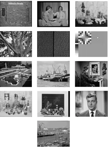
Figure1: Images used for training.
3. RESULTS
To assess the performance of the noise estimation processes, a series of simulations was conducted. The three meth-ods for noise estimation presented inSection 2were imple-mented along with MAD. Those methods that needed train-ing were trained on a set of 13 images (Figure 1). The per-formance of the methods was then evaluated using a
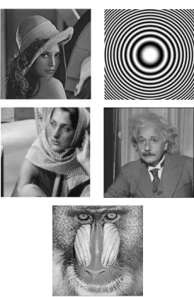
selec-tion of five images (Figure 2).1 Note that the training and test sets contained no common images. Gaussian noise was added to each of the five images using six different noise lev-els. The noise was estimated using only the highest frequency
1Training and test sets of images are available athttp://www.soton.ac.uk/
Figure2: Images used for testing.
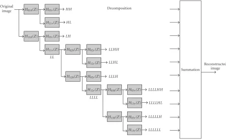
(smallest scale) wavelet component. The filter bank used for the wavelet decomposition is showed in Figure 3 and the coefficients described in (10),2
H11h= [1, 2, 1]
4 , H01h=
[−1, 2,−1]
4 ,
H11v=H11hT, H01v=H01hT, H12h= [1, 0, 2, 0, 1]4 , H02h=[−1, 0, 2, 0,4 −1],
H12v=h12hT, h02v=h02hT, H13h=
[1, 0, 0, 0, 2, 0, 0, 0, 1]
4 ,
H03h=[−1, 0, 0, 0, 2, 0, 0, 0,4 −1], H13v=H13hT, H03v=H03hT.
(10)
2The filter bank used for the wavelet decomposition is extensively
de-scribed in [3].
The mean squared error between the estimated noise vari-ance and the true varivari-ance of the added noise is computed; the results are presented in Tables1and2.
Decomposition Original
image H01h(Z) H01v(Z) HH
H11v(Z) HL
H11h(Z) H01v(Z) LH
H11v(Z) H02h(Z) H02v(Z) LLHH
LL
H12v(Z) LLHL
H12h(Z) H02v(Z) LLLH
H12v(Z) H03h(Z) H03v(Z) LLLLHH
LLLL
H13v(Z) LLLLHL
H13h(Z) H03v(Z) LLLLLH
H13v(Z) LLLLLL
Summation
Reconstructed image
Figure3: Filter bank used for the wavelet decomposition.H0mhandH1mhare the horizontal decomposition filters for decomposition level
handH0mvandH1mvare the vertical decomposition filters for decomposition levelh. The reconstruction is achieved by summing of the
components.
Table 2 compares the performance of the three new methods with those of the MAD method and with re-spect to the five images. The mean squared error is com-puted over the six noise levels. The cdf method achieves the best performances for three images (A, B, and C), the performances of the MAD and moment matching meth-ods are superior, respectively, for images D and E. In gen-eral, again the two training-based methods achieve bet-ter performance than the moment matching technique or MAD.
We believe that the poor performance of the moment matching method (third column) can be attributed to the inadequacy of the Laplacian distribution for modelling the underlying image. This has been verified by comparing the mean squared error between synthetically generated images with optimal3Laplacian distribution and the image compo-nent distribution (sixth column). The ratio between the val-ues in the third and sixth columns and in the same row is almost constant and this demonstrates that performances of the moment matching method are strongly related to the dis-crepancy between optimal (Laplacian distribution) and real image components.
3The parameters of the Laplacian distribution were selected to minimise
the MSE between synthetic image and image component.
We also believe that the comparatively poor performance of MAD (second column) is due to the fact that it assumes that there is zero image contribution in the component being examined. The last column ofTable 2lists the standard devi-ation of the image component. Comparing the second and last columns, the relation between the MAD performance and the standard deviation of the image component contri-bution is clear.
4. CONCLUSIONS
Table1: Mean squared errors for noise standard deviation estimates computed over 5 images.
Standard deviation
MAD Moment matching Trained moments cdf
of synthetic noise
5 3.49 2.49 2.35 2.73
7 3.01 2.36 1.91 1.86
9 2.63 2.13 1.59 1.55
11 2.33 1.97 1.38 1.40
13 2.08 1.76 1.37 0.46
15 1.84 1.62 1.31 0.43
Overall mean 2.56 2.06 1.65 1.41
Table2: Mean squared errors for noise standard deviation estimates computed over 6 noise levels (columns 2–5); mean squared error
between image component and synthetically generated image with optimal Laplacian distribution (column 6); and standard deviation of the image component (column 7).
Image MAD Moment matching Trained moments cdf MSE (IC−IL) STDIC
Image A 2.75 2.89 0.84 0.34 1.18 8.14
Image B 1.27 1.32 1.25 1.00 0.62 2.57
Image C 1.95 3.25 0.98 0.71 1.45 3.49
Image D 0.83 1.22 1.52 1.73 0.47 1.67
Image E 5.98 1.62 3.68 3.26 0.83 11.11
Overall mean 2.56 2.06 1.65 1.41 — —
of the class of the video images and completely disjoint from the set used for testing the methods and comparing the results. For the large majority of the images and noise levels considered, the training-based methods demonstrated their ability to offer superior performance. The advantages and disadvantages of the model-based techniques, such as the MAD and the novel model proposed here, are also dis-cussed.
The results showed in this paper need to be generalised using larger sets of test images and different range noise lev-els. The techniques proposed seem also to be suitable for other classes of images and for non-spatially white Gaussian noise distributions. A desirable development of this work could focus on these aspects.
ACKNOWLEDGMENT
We would like to gratefully acknowledge the financial sup-port of Snell and Wilcox Ltd. in conducting this work and would particularly like to thank Martin Weston for his many comments and suggestions.
REFERENCES
[1] D. L. Donoho, “De-noising by soft-thresholding,”IEEE Trans-actions on Information Theory, vol. 41, no. 3, pp. 613–627, 1995.
[2] A. Bruce, D. Donoho, and H. Gao, “Wavelet analysis [for sig-nal processing],” IEEE Spectrum, vol. 33, no. 10, pp. 26–35, 1996.
[3] A. De Stefano, Wavelet based reduction of spatial video noise, Ph.D. thesis, ISVR, University of Southampton, Southamp-ton, UK, 2000.
[4] M. R. Banham and A. K. Katsaggelos, “Spatially adaptive wavelet-based multiscale image restoration,” IEEE Trans. Im-age Processing, vol. 5, no. 4, pp. 619–634, 1996.
[5] M. Lang, H. Guo, J. E. Odegard, C. S. Burrus, and R. O. Wells Jr., “Noise reduction using an undecimated discrete wavelet transform,” IEEE Signal Processing Letters, vol. 3, no. 1, pp. 10–12, 1996.
[6] D. L. Donoho and I. M. Johnstone, “Ideal spatial adaptation by wavelet shrinkage,”Biometrika, vol. 81, no. 3, pp. 425–455, 1994.
[7] D. L. Donoho and I. M. Johnstone, “Wavelet shrinkage: asymptopia?,” Journal Royal Statistics Society B, vol. 57, no. 2, pp. 301–369, 1995.
[8] E. P. Simoncelli, “Bayesian denoising of visual images in the wavelet domain,” inBayesian Inference in Wavelet-Based Models, P. Muller and B. Vidakovic, Eds., vol. 141 ofLecture Notes in Statistics, pp. 291–308, Springer-Verlag, New York, NY, USA, 1999.
[9] H. Y. Gao and A. G. Bruce, “WaveShrink with firm shrinkage,” Statistica Sinica, vol. 7, no. 4, pp. 855–874, 1997.
[10] R. R. Coifman and D. L. Donoho, “Translation-invariant de-noising,” inWavelets and Statistics, A. Antoniadis and G. Op-penheim, Eds., vol. 103 ofLecture Notes in Statistics, pp. 125– 150, Springer-Verlag, New York, NY, USA, 1995.
[11] A. De Stefano, P. R. White, and W. B. Collis, “An innova-tive approach for spatial video noise reduction using a wavelet based frequency decomposition,” inProc. IEEE International Conference on Image Processing (ICIP ’00), vol. 3, pp. 281–284, Vancouver, British Columbia, Canada, September 2000. [12] A. De Stefano, P. R. White, and W. B. Collis, “Selection of
components using Bayesian estimation,” inProc. 5th IMA International Conference on Mathematics in Signal Processing, Warwick, UK, December 2000.
[13] G. Strang and T. Nguyen,Wavelets and Filter Banks, Wellesley Cambridge Press, Wellesley, Mass, USA, 1996.
[14] M. Jansen and A. Bultheel, “Multiple wavelet threshold esti-mation by generalized cross validation for images with corre-lated noise,” IEEE Trans. Image Processing, vol. 8, no. 7, pp. 947–953, 1999.
[15] Y. Xu, J. B. Weaver, D. M. Healy Jr., and J. Lu, “Wavelet trans-form domain filters: a spatially selective noise filtration tech-nique,” IEEE Trans. Image Processing, vol. 3, no. 6, pp. 747– 758, 1994.
[16] S. Mallat and W. L. Hwang, “Singularity detection and pro-cessing with wavelets,”IEEE Transactions on Information The-ory, vol. 38, no. 2, pp. 617–643, 1992.
[17] M. Malfait and D. Roose, “Wavelet-based image denoising us-ing a Markov random field a priori model,”IEEE Trans. Image Processing, vol. 6, no. 4, pp. 549–565, 1997.
[18] M. R. Banham and A. K. Katsaggelos, “Spatially adaptive wavelet-based multiscale image restoration,” IEEE Trans. Im-age Processing, vol. 5, no. 4, pp. 619–634, 1996.
[19] P. Moulin and J. Liu, “Analysis of multiresolution image de-noising schemes using generalized Gaussian and complexity priors,”IEEE Transactions on Information Theory, vol. 45, no. 3, pp. 909–919, 1999.
[20] D. Wei and C. S. Burrus, “Optimal wavelet thresholding for various coding schemes,” inProc. IEEE International Confer-ence on Image Processing (ICIP ’95), vol. 1, pp. 610–613, Wash-ington, DC, USA, October 1995.
[21] T. R. Downie and B. W. Silverman, “The discrete mul-tiple wavelet transform and thresholding methods,” IEEE Trans. Signal Processing, vol. 46, no. 9, pp. 2558–2561, 1998. [22] S. Mallat, Wavelet Tour of Signal Processing, Academic Press,
San Diego, Calif, USA, 1998.
[23] C. Taswell, “Experiments in wavelet shrinkage denoising,” Journal of Computational Methods in Sciences and Engineering, vol. 1, no. 2s-3s, pp. 315–326, 2001.
[24] C. Taswell, “The what, how, and why of wavelet shrinkage denoising,” IEEE Computing in Science and Engineering, vol. 2, no. 3, pp. 12–19, 2000, invited paper.
[25] A. Papoulis,Probability, Random Variables, and Stochastic Pro-cesses, McGraw-Hill, New York, NY, USA, 1991.
[26] H. L. Van Trees, Detection, Estimation, and Modulation The-ory, Part I, John Wiley & Son, New York, NY, USA, 2001.
A. De Stefanois Distance Learning Coor-dinator for the Master Training Packages at the Centre of Biomedical Signal Processing, Institute of Sound and Vibration Research (ISVR), University of Southampton, UK. He received the Electronics Engineering de-gree in biomedical sciences, the CEng qual-ification from the University of Federico II in Naples, Italy, and the Ph.D. degree from the ISVR at the University of Southampton,
UK. His research interests include wavelet-based noise reduction and image enhancement, biomedical signal processing, implemen-tation of distance learning packages for biomedical subjects, tech-niques for EMG analysis during walking of pathological children, and mechanical models for speech design. He has over 20 publica-tions in journals and international conferences.
P. R. Whiteis currently a Senior Lecturer in the Institute of Sound and Vibration Re-search, the University of Southampton. He attained his degree in applied mathemat-ics from Portsmouth Polytechnic in 1985, whereupon he joined the ISVR to study for his Ph.D. In 1988, he was made a Lecturer in ISVR, finally completing his Ph.D. in 1992. In 1998, he was made a Senior Lecturer. The basic signal processing techniques that have
formed the basis of this work include time-frequency analysis, non-linear systems, adaptive systems, detection and classification algo-rithms, higher-order statistics, and independent component anal-ysis. The application areas which he has considered include im-age processing, underwater systems, condition monitoring, and biomedical applications. He has published more than 130 papers in the field, approximately 35 of which appearing in referred journals or as chapters in books. He is a Member of the Editorial Board of the Journal of Condition Monitoring and Diagnostic Engineering Management (COMADEM) and is a Member of the IEEE.
W. B. Collishas been Algorithms Engineer at the Foundry since December 2000. Prior to joining the Foundry, Collis led the algo-rithms team at Snell & Wilcox for 5 years working on standards conversion, motion estimation, archive restoration, and filter design. During this period he also devel-oped the Flo-Mo retiming software used in the pioneering “bullet time” sequences in the filmThe Matrix. Collis graduated with