Bayesian Optimization in Machine Learning

(1)

Title: Bayesian Optimization in Machine Learning

Author: José Jiménez Luna

Advisor: Josep Ginebra Molins

Department: Estadística i Investigació Operativa

University: Universitat Politècnica de Catalunya

Academic year: 2016-2017

Interuniversity Master

in Statistics and

Operations Research

UPC-UB

(2)

Universitat Polit`

ecnica de Catalunya

Facultat de Matem`

atiques i Estad´ıstica

Master’s Thesis

Bayesian optimization in machine learning

Jos´

e Jim´

enez Luna

supervised by

Josep Ginebra

Departament Estad´ıstica i Investigaci´o Operativa. ETSEIB.

(3)

(4)

Abstract

Bayesian optimization has risen over the last few years as a very attractive approach to find the optimum of noisy, expensive to evaluate, and possibly black-box functions. One of the fields where these functions are common is in machine-learning, where one typically has to fit a particular model by minimizing a specified form of loss. In this Master’s thesis we first focus on reviewing the most recent literature on Gaussian Processes as well as Bayesian optimiza-tion methods, then we benchmark said methods against several real case machine-learning scenarios and lastly we provide open source software that will allow researchers to apply these strategies in other problems.

Keywords: machine-learning, bayesian, optimization

(5)

(6)

There ain’t no such thing as a free lunch.

Friedman. M. (1975)

(7)

(8)

5.6 Future work . . . 83 Appendices 87 A Examples code 89 A.1 drawGP.py . . . 89 A.2 sineGP.py . . . 89 A.3 covzoo.py . . . 90 A.4 hyperopt.py . . . 91 A.5 acqzoo.py . . . 92 A.6 integratedacq.py . . . 93 A.7 bayoptwork.py . . . 94 A.8 sineopt.py . . . 94 A.9 rastriginopt.py . . . 95 B Testing code 99 B.1 utils.py . . . 99 B.2 modaux.py . . . 102 B.3 testing.py . . . 105

(10)

Chapter 1

Organization of this work

1.1

Introduction

This Master’s thesis has three different and complimentary aims:

• The first objective of the thesis is to provide the reader with an introduction to Gaussian Process regression and Bayesian optimization. While there are vast pieces of work for both Gaussian Processes and Bayesian Optimization, this work aims to bridge the gap between them. I try to cover as much literature as needed to provide the reader with enough background to understand and implement the theoretical work presented here. Explanations are accompanied by comprehensive coding implementations and examples that help understand the material.

• To show the Bayesian Optimization framework works in several real-world machine learning tasks. This is done by selecting several datasets related to open computational chemistry problems, fol-lowing said methodology and finally comparing its performance to other already existing strategies.

• Finally, to write a complete software package for users to apply Bayesian Optimization in their research. This comes in the form of a Python (>3.5) package named pyGPGO. The code can either be obtained through its GitHub repository https://github.com/hawk31/pyGPGO or the Python Package Index (PyPI). The entire software package is MIT licensed. All the examples and code snippets throughout this manual are based on this software. While certainly there are a couple implementations of Global Optimization software in Python, the software developed here is modular, easy to use and requires minimal dependencies, while still being feature-wise competitive. We begin by describing the title of this thesis. Bayesian Optimization focuses on the global optimiza-tion of a funcoptimiza-tionf :Rn→Rover a compact setA. The problem can be formalized as:

max

x∈Af(x) (1.1)

Most optimization procedures (local based ones such as gradient ascent, for example) assume that the function f is closed-form, that is, it has an analytical expression, that it is convex, with known first or second order derivatives or cheap to evaluate. Bayesian optimization focuses on all these problems proposing a very elegant solution. By the use of a surrogate model, a Gaussian Process, a Bayesian optimization procedure can help find the global minimum of non-necessarily convex, expensive functions that are expensive to evaluate. These methods shine also where there is no closed-form expression to evaluate or derivatives.

At the same time, in machine learning (or statistical learning), we are usually interested in minimizing a loss functionL over a subset of data. These losses can take many forms, e.g. when doing regression, a typical loss might be the mean squared error between predictions and observed values on a holdout test set.

(11)

10 CHAPTER 1. ORGANIZATION OF THIS WORK L(y,yˆ) = 1 n X i (yi−yiˆ)2 (1.2)

In binary classification, for example, a very popular choice is the logarithmic loss:

L(y,yˆ) =−1 n =

X i

(yilog( ˆyi) + (1−yi) log(1−yiˆ)) (1.3) Notice in any case, that these losses are typically defined in a subset ofR. In the work described here we

focus on the supervised setting of machine learning. Depending on the problem at hand, even evaluating these losses can be very expensive from a computational point of view. This may have to do with the machine learning algorithm used or dataset size. These machine learning algorithms typically have

hyperparameters that have to be tuned in a sensible way to get the best performance possible out of these models. In the machine learning community it is common for practitioners to perform hyperparameter grid lookups or randomized searches to reach reasonable solutions. However, with the advent of big-data and more computationally hungry strategies, the training of a single model could already take substantial resources in terms of CPU cycles or memory, that is translated in higher wall-clock waiting times. Therefore we would like to have a more efficient and cheap way to optimize these hyperparameters. Bayesian optimization will let us do that by proposing the next candidate hyperparameter set x to evaluate according to several criteria.

1.2

Organization of the thesis

The whole thesis is organized in 5 self-contained chapters. First, all the theoretical work is presented, for both Gaussian Processes and Bayesian optimization, then benchmarking of the method is presented, and finally we describe the developed piece of software. I briefly describe the content of each chapter here:

Chapter 2focuses on a swift but thorough introduction to regression problems using Gaussian

Pro-cesses. These are the surrogate models we will use for Bayesian Optimization in Chapter 3. We will mostly cover the theory behind them from a functional point of view. We will also explain different covariance functions and their role in these models. Special attention is given to different approaches towards covariance hyperparameter treatment. Further theoretical aspects are also discussed.

Chapter 3is about the main topic in this work, Bayesian Optimization. Once we have laid down

all the foundations of Gaussian Processes, we can start explaining the theory of Bayesian optimization using these as surrogate models. The role of several acquisition functions, i.e. functions that will propose the next point to evaluate will be thoroughly discussed, as well as their advantages or disadvantages. Different modelling choices are then further presented. References on this chapter will be very diverse, as I will try to summarize several recent publications on the field.

Chapter 4covers experiments using the software provided alongside this manual. These are mostly

mid-sized regression or classification problems where we will compare the performance of Bayesian Op-timization of hyperparameters with several regressors/classifiers with other strategies, such as random search. Most of these datasets are related to the experimental sciences, in particular chemistry, and some of them were used for other benchmarking purposes in other studies.

Chapter 5holds no theoretical content nor testing content. It will cover technical explanations of

(12)

Chapter 2

Gaussian Process regression

In this chapter we will focus on regression problems. Assume we have some labelled data

D={(xi, yi)|i= 1, . . . , n}, (2.1) wherex is a vector of covariates andy denotes a continuous objective variable. We wish to learn a predictive distribution over new values of ygivenx, so that we can make predictions and inference over these. In practice, for simplicity we write thatD={X,y}, whereX is our predictor matrix.

One can interpret a Gaussian Process in several ways. The most widely known is the function space view, which is the one we will cover first here and the one we will assume for the rest for the thesis. In this view, we consider a Gaussian Process to be a stochastic process, hence, a distribution over functions, instead of over values. Inference takes place directly in this space. For completeness, we will also pro-vide a weight-space view second, that might be more appealing to readers familiar with Bayesian linear regression.

2.1

A function space view for Gaussian Processes

We start by formally defining a Gaussian Process:

Definition 1 A Gaussian Process is a collection of random variables, any finite number of which have

a joint Gaussian distribution. This process is totally defined by two functions. Its mean function:

m(x) =E[f(x)] (2.2)

and its covariance function:

k(x,x0) =E[(f(x)−m(x)) (f(x0)−m(x0))] (2.3)

We say thatf is a Gaussian Process with mean m(x)and covariance functionk(x, x0)and write:

f(x)∼ GP(m(x), k(x,x0)) (2.4)

In practice, for simplicity we will take m(x) = 0, but this can be specified otherwise. Further-more, a Gaussian Process fulfils the marginalization property, that is to say that if the the GP specifies (y1, y2)∼ N(µ,Σ) then it follows thaty1 ∼ N(µ1,Σ11). A Gaussian multivariate distribution is just a

finite index set of a given Gaussian Process.

Define then a covariance function, such as thesquared exponential kernel, written as:

k(x,x0) = exp −1 2|x−x 0_|2 (2.5) 11

(13)

12 CHAPTER 2. GAUSSIAN PROCESS REGRESSION

Figure 2.1: Three sampled Gaussian Process priors using the Squared Exponential kernel.

0

1

2

3

4

5

6

x

3

2

1

0

1

2

y

Sampled GP priors from Squared Exponential kernel

GP sample 1

GP sample 2

GP sample 3

where |.| denotes the standard L2 norm. Most of the covariance functions that we will see here are

a function of this norm, therefore it is much more comfortable to write r =|x−x0|and therefore the squared exponential kernel becomes:

k(r) = exp −1 2r 2 (2.6)

It is straightforward to draw samples from a Gaussian Process. In particular, since we work with a finite number of points, choose an arbitrary number of examplesX∗and compute the squared exponential

kernel (assumingm(x) =0). Then the procedure is simplified to sampling from the following multivariate Gaussian:

f∗∼ N(0, K(X∗, X∗)) (2.7)

We have written a very simple script to illustrate this point, which is available in Appendix A.1, pro-ducing Figure 2.1. Most of the code examples presented throughout the rest of the text were programmed using pyGPGO, the software developed alongside this thesis.

Before we move on, notice that the drawn functions in Figure 2.1 seem to have a characteristic length-scale. This can be interpreted as the distance one has to move in input space before the function value changes significantly. By default, the squared exponential kernel uses a characteristic length-scale of 1 (l = 1). To change this behaviour, it is sufficient to considerr/linstead of rin Equation 2.6. This can be thought as an hyperparameter to optimize. We will return to this problem in Section 2.5.

(14)

2.2. A WEIGHT SPACE VIEW FOR GAUSSIAN PROCESSES 13

2.2

A weight space view for Gaussian Processes

In this section I will try to draw connections between Bayesian linear regression [2] and Gaussian Pro-cesses, through the use of kernel functions.

2.2.1

Standard Bayesian linear regression

A Bayesian linear regression model with Gaussian error can be formulated as:

y =XTw+ (2.8)

where we typically assume∼ N(0, σ2

n). This noise assumption directly implies a Gaussian likelihood,

thus it can be easily proven that:

p(y|X,w)∼ N(XTw, σ2nI) (2.9)

Assume now a Gaussian prior on the weightsw:

w∼ N(0,Σp) (2.10)

We are interested now on the posterior distribution of w, given both X and y, and assuming the model in Equation 2.8, that is:

p(w|y, X) = p(y|X,w)p(w)

p(y|X) (2.11)

One can solve this problem by means of sampling procedures like Markov Chain Monte Carlo, but in this particular case, there is a closed-form solution. It can be proven that:

p(w|X,y)∼ N ₁ σn n A−1Xy, A−1 (2.12) where A = σ−2_XXT _{+ Σ}−1

p . Notice that a simple MAP (maximum a posteriori) estimate of the

weights can be obtained by just computing the mean of this distribution. Now, to make predictions for a particular test casex∗, we average over all possible parameter values, hence we get a whole predictive

distribution. Again, it can be shown that:

f∗|x∗, X,y∼ N ₁ σ2 n x∗TA−1Xy,x∗TA−1x∗ (2.13)

2.2.2

Kernel functions in feature space

We have presented a very simple Bayesian approach to linear regression in the previous section. While useful, it lacks expressiveness due to its linearity. A very simple idea is to project this data into a higher dimension, where it may be more easily separated by a linear model of this sort. This is known as using the kernel trick [4]. We can do this through a covariance (or kernel) functionφ(x). Note by Φ(X) the aggregation of columns after computing this kernel function in the entire dataset at hand.

The model becomes now:

f(x) =φ(x)Tw (2.14)

where we assume the same prior overw as in Equation 2.10. All the math presented in the previous section applies here, just placing φ(x) instead ofx. The predictive distribution overy becomes now, for example: f∗|x∗, X,y∼ N ₁ σ2 n φ(x∗)TA−1Φy, φ(x∗)TA−1φ(x∗) (2.15)

(15)

14 CHAPTER 2. GAUSSIAN PROCESS REGRESSION

where for simplicity we have written Φ = Φ(X) andA=σ−2

n ΦΦT+ Σ−p1. The predictive distribution

needs to invertN×N matrix. Equation 2.15 can be rewritten as:

f∗|x∗, X,y∼ N

φ∗TΣpΦ(K+σn2I)−1y,φ∗Σpφ∗−φ∗TΣpΦ(K+σn2I)−1ΦTΣpφ∗

(2.16) where we have again simplified notation by φ∗ = φ(x∗) and K = ΦTΣpΦ. Now notice that the

entries ofKfor both train and test set are of the formφ(x∗T)Σpφ(x∗). We have implicitly defined now a

covariance function of the formk(x,x0) =φ(x∗T)Σpφ(x∗). This is in fact an inner product with respect

to Σp. That is if we define ψ(x) = Σ

1/2

p (x), then a simple dot product representation of a covariance

function is:

k(x,x0) =ψ(x)Tψ(x0) (2.17)

where Σ1p/2 can be defined by means of a singular value decomposition. We then replace the original

feature vectors by these dot products,lifting to a higher space. In the next Section, we will perform the same calculations detailed here, but using the function space view that will be used throughout the rest of the text.

2.3

Prediction using a Gaussian Process prior

In this particular section, arguably the most important one in the chapter, we will learn how to incor-porate the knowledge of training data D ={(xi, yi)|i= 1, . . . , n} into our Gaussian Process to obtain

a posterior predictive distribution. We will start considering the case that we have a noiseless function, that is to say, whenσ2

n= 0. Let us defineK(X, X∗), the covariance function evaluated on train and test

points, K(X, X) the covariance function evaluated at only the training points,K(X∗, X∗) equivalently

defined for the test values. Notice the last two have to be square matrices by definition. Let us also use the following theorem:

Theorem 1 Let xandy be jointly Gaussian:

x y ∼ N µx µy , A C CT _B (2.18) Thenx|y∼ µx+CB−1(y−µy), A−CB−1CT

Similarly as in Equation 2.7, assume thatf andf∗are jointly Gaussian:

f f∗ ∼ N 0, K(X, X) K(X, X∗) K(X∗, X) K(X∗, X∗) (2.19) We are interested now in the distribution off∗|f. Simply applying Theorem 1, we can obtain:

f∗|f ∼ N K(X∗, X)K(X, X)−1f, K(X∗, X∗)−K(X∗, X)K(X, X)−1K(X, X∗) (2.20)

This covers all the basics for a Gaussian Process regression model. Notice that now we have a com-plete predictive distribution over test valuesf∗, and this provides us with plenty of choices. For example,

one could obtain an estimate of this function by drawing samples from a multivariate normal with the computed posterior parameters, or obtain a MAP estimate using the posterior mean.

Let us now consider the scenario where observations are not noise-free, that is, each time the function is queried it comes with i.i.d Gaussian error with mean 0 and varianceσ2

n>0. Assume now the following

prior on the noisy observations:

(16)

2.3. PREDICTION USING A GAUSSIAN PROCESS PRIOR 15

Following the exact operations as before, but taking into account this new term, we got the following joint distribution: y f∗ ∼ N 0, K(X, X) +σ2 nI K(X, X∗) K(X∗, X) K(X∗, X∗) (2.22) And conditioning againf∗ ony, we obtain our final predictive distribution:

f∗|y∼ N(f∗, Cov(f∗)) (2.23) where now: f∗=K(X∗, X) K(X, X) +σn2I −1 y Cov(f∗) =K(X∗, X∗)−K(X∗, X) K(X, X) +σn2I −1 K(X, X∗) (2.24)

It will probably be useful to note that a Gaussian Process model can be written in terms of a Bayesian hierarchical model, since:

y|f ∼ N(f, σn2I)

f|X ∼ N(0, K(X, X)) (2.25)

In fact, one can also assume other priors, even overσ2

n. This representation may help us understand

the introduction of the marginal likelihood. This marginal likelihood in a Gaussian Process setting is defined as:

p(y|X) =

Z

p(y|f, X)p(f|X)df (2.26)

Using the results from Equations 2.25 we can derive the integral analytically to obtain:

logp(y|X) =−1 2y T₍_K₊_σ2 nI) −1_y₋1 2log|K+σ 2 nI| − n 2 log 2π (2.27)

where we write K = K(X, X) for simplicity. Notice this result is equivalent to the log-density of

y∼ N(0, K+σn2I). We have now all the necessary ingredients to lay down pseudo-code for the

imple-mentation of a Gaussian Process regressor, as presented in Algorithm 7. It makes use of several tricks for computational stability, such as a Cholesky decomposition and several linear system of equations to avoid directly inverting matrices.

Algorithm 1 Gaussian regressor pseudo-code.

1: functionGaussianProcess(X,y, k,σ2_n,x∗) 2: L←chol(K+σ_n2I) 3: α←linsolve LT,linsolve(L,y) 4: f∗←k∗Tα 5: v←linsolve(L,k∗) 6: _V[f∗]←k(x∗,x∗)−vTv 7: logp(y|X)← −1 2y T_α₋P ilogLii− n 2log 2π 8: end function

pyGPGO includes an implementation of a Gaussian Process regressor under thesurrogates.GaussianProcess

(17)

16 CHAPTER 2. GAUSSIAN PROCESS REGRESSION

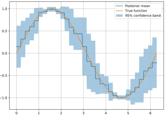
Figure 2.2: A fitted Gaussian Process regressor to samples of the sine function.

0

1

2

3

4

5

6

1.5

1.0

0.5

0.0

0.5

1.0

1.5

Posterior mean

True function

95% confidence band

2.3.1

A toy example of Gaussian Process regression

Now that we have both the algorithm and the tools at hand, it may be interesting how a Gaussian Process regressor behaves with a toy example. We try to approximate a simple sine function in the interval [0,2π], and plot both the posterior mean and a 95% confidence band using the posterior variance of the fitted process. The code in Appendix A.2 produces Figure 2.2.

2.3.2

Picking a winner

In the previous section we have shown how to compute predictive posterior distribution for function outputs y∗ given a new inputx∗. These are given by a Gaussian distribution with a certain mean and

variance. In plenty of production settings, however, it is more common to provide a single value, or estimate yguess that is optimal in some sense. To define a sense of optimality, define a loss function

L(ytrue, yguess). This, defines a penalty incurred by taking the decision to useyguess when the true value

is ytrue. For example, this could be the mean square or mean absolute error function. In the Bayesian

setting, there is no clear mention of a loss function in any stage. In the frequentist setting, however, a model is usually trained by minimizing this loss. Furthermore, there is a clear separation between loss and likelihood in the Bayesian setting, the latter used for training, with prior information. The loss function however only captures the consequences of making a single specific choice given a true state.

Again, we would like to somehow pick a winner yguess that minimizes our loss. Without knowing

(18)

2.4. ON COVARIANCE FUNCTIONS 17

RL(yguess|x∗) =

Z

L(y∗, yguess)p(y∗|x∗,D)dy (2.28)

Our optimal value is the one that minimizes this expected loss:

yoptimal|x∗= arg min

yguess

RL(yguess|x∗) (2.29)

It can be proven that the valueyguess that minimizes Equation 2.29 for the absolute loss function is

the median ofp(y∗|x∗,D). For the squared loss function, it is the mean of the same distribution. Since

in our case we are dealing with the Gaussian distribution, median and mean coincide, and the most reasonablewinner will therefore be the specific value of the posterior mean.

2.4

On covariance functions

A covariance function [11], like the squared exponential kernel that we have been using as a example throughout the chapter encodes our assumptions of similarity between inputs fromx. We assumesimilar

items in input space to have similar values of the target value y. Not all functions of xand x0 can be defined as covariance function. Covariance functions (though not all) tend to satisfy different properties:

• Weak stationarity. A covariance function is said to be weakly stationary if it is a function ofx−x0. That is to say that it is invariant to translations in the input space. Most of the covariance functions we will see fall into this category.

• Isotropy. A covariance function is said to be isotropic if it is only function of |x−x0|. Therefore, every isotropic covariance function is stationary.

• Dot-product. Some covariance functions are functionals of the dot-product|xT_x0_|_{. These kernels,}

while invariant to rotations are not invariant to translations.

There is an excellent theoretical analysis of covariance functions in [9]. We will not cover this here since it falls beyond the scope of this thesis. However, we will start providing examples of the most common covariance functions. All covariance functions described here are implemented in the software developed alongside this thesis, pyGPGO, in thecovfuncmodule. We will describe their functionality in Section 5.1. The Squared Exponential covariance function is the one that we have been using so far. It is also arguably the most used in practice. It takes the general form:

kSE(r) = exp −r 2 2l2 (2.30) wherelis the parameter controlling its characteristic length-scale. It is useful to define these functions in terms ofr since we can abstract this calculation to another function.

TheMat´ern class of covariance functions [5] takes the form:

kMatern(r) = 21−ν Γ(ν) √ 2νr l !ν Kν √ 2νr l ! (2.31) withν, l >0 andKν is a modified Bessel function of the second kind [1]. Simple functional forms can be obtained whenνis half integer, that isν =p+ 1/2 forpnon-negative integer. In particular, ifν= 1/2, we obtain the a simple exponential kernel and if we take limitν → ∞we obtain the squared exponential covariance function. Popular values are ν= 3/2 (once-differentiable) andν= 5/2 (twice-differentiable). Theγ-exponential covariance function, of which the squared exponential is a special case, takes the general form:

(19)

18 CHAPTER 2. GAUSSIAN PROCESS REGRESSION kGE(r) = exp −r l γ (2.32) for 0< γ≤2.

TheRational Quadratic covariance function can be written as:

kRQ(r) = 1 + r 2 2αl2 −α (2.33) withα, l >0. This covariance function can be seen as a scale mixture of squared exponential kernels with different length scales.

ThearcSin kernel is an example of a dot product covariance function, therefore non-stationary:

karcSin(x,x0) = 2 πsin −1   2xΣx0 q (1 + 2xT_Σ_x_{)(1 + 2}_x0T Σx)   (2.34)

where Σ is some semidefinite positive matrix. Normally, these are the covariance functions that are used for the noiseless case of observation, that is, we know precisely that f(xi) = yi, i = 1. . . n. In

general, our covariance functions will take the form:

ky(xp,xq) =σf2k(xp,xq) +σn2δpq (2.35)

whereσ2

f is the signal variance, and controls the overall scale of our covariance matrix,σ

2

n is the noise

variance andδpq is a Kronecker delta function. Notice we note nowky instead ofkto account for noisy

observations. In practice, all covariance function internal parameters plus nσ2

n, σf2 o

can be considered unknowns of our particular problem. Several different treatments of hyperparameters can be considered, for example, one may choose to fix them manually, try to optimize them in a maximum-likelihood fashion (Section 2.5) or take the full Bayesian approach and marginalize over them (Section 2.6.3).

2.4.1

Visualizing different covariance functions

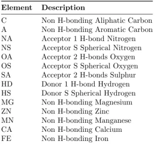
We have seen plenty of covariance function specifications in the last section. Remember that these control the degree ofsimilarity between input points. As an exercise, it would be good to recreate the same sine function example that we saw before, using four different stationary different covariance functions. The choice of parameters is the default one in pyGPGO. The script detailed in Appendix A.3 below produces Figure 2.3.

2.5

Hyperparameter optimization

As seen in the previous sections, different covariance functions have different hyperparameters. These control how the kernel measures similarity among different instances of x. So far, we have chosen these hyperparameters according to those set default in pyGPGO, but one may want to choose these according to training data. Depending on the situation, good parameter choices should lead to better models, either in terms of accuracy or interpretability. There are several ways to select these hyperparameters, by opti-mizing the marginal log-likelihood or via cross-validation. A full Bayesian treatment of hyperparameters is discussed in Section 2.6.3.

(20)

2.5. HYPERPARAMETER OPTIMIZATION 19

Figure 2.3: Behaviour of different stationary covariance functions with the default parameters in pyGPGO. 0 1 2 3 4 5 6 1.0 0.5 0.0 0.5 1.0 Squared Exponential (l = 1) 0 1 2 3 4 5 6 1.5 1.0 0.5 0.0 0.5 1.0 1.5 Matern ( = 1, l = 1) 0 1 2 3 4 5 6 1.5 1.0 0.5 0.0 0.5 1.0 1.5 Gamma Exponential ( = 1, l = 1) 0 1 2 3 4 5 6 1.0 0.5 0.0 0.5 1.0 Rational Quadratic ( = 1, l = 1) Posterior mean True function 95\% confidence band

(21)

20 CHAPTER 2. GAUSSIAN PROCESS REGRESSION

2.5.1

Type II Maximum Likelihood

This is the empirical Bayes [10] analytical approach to optimizing hyperparameters. One may quickly notice that Gaussian Processes are non-parametric models, in the sense that apart from the quantities set in the covariance functions, there is nothing else to optimize for. First we will provide a small background on Bayesian model selection. Assume that we have a modelHi withparameters w,hyperparameters θ,

and we have some training dataX,y. The posterior over the parameters is given by Bayes’s theorem:

p(w|y, X,θ,Hi) =

p(y|X,w,Hi)p(w|θ,Hi) p(y|X,θ,Hi)

(2.36) where p(y|X,w,Hi) is the likelihood, p(w|θ,Hi) our prior distribution over the parameters and p(y|X,θ,Hi) is called theevidence or marginal likelihood. Notice that this last quantity is nothing but

the integral over parameterw space of the numerator in Equation 2.36.

We can do the same at the next level of inference for the hyperparameters. The posterior of hyper-parameters is defined as:

p(θ|y, X,Hi) =

p(y|X,θ,Hi)p(θ|Hi) p(y|X,Hi)

(2.37) where nowp(θ|Hi) is our prior over hyperparameters. We are interested however in optimizing the

denominator in Equation 2.37 with respect to the hyperparameters. Typically, in Bayesian inference to perform the kind of integrals presented before, one has to resort to sampling procedures related to Markov Chain Monte Carlo, such as the Gibbs sampler. In the case of Gaussian processes, all computations are analytically tractable. In fact, the expression of the marginal likelihood was presented in Section 2.3. We reproduce the expression here for completeness:

logp(y|X) =−1 2y T₍_K₊_σ2 nI)− 1_y −1 2log|K+σ 2 nI| − n 2 log 2π (2.38)

For typical local optimization methods to work fairly well, we may also need an specification of the derivative of the log-marginal likelihood w.r.t. the hyperparameters.

∂ ∂θj logp(y|X,θ) = 1 2y T_K−1∂K ∂θjK −1_y₋1 2tr K−1∂K ∂θj (2.39) where∂K ∂θj

denotes the derivative of the selected covariance function, evaluated at each pair of instances of the training set. For optimization, one may choose to make use of this expression or not, depending on both of the optimization algorithm (gradient ascent, L-BFGS-B...) or on the cost of evaluation of the derivative. In pyGPGO, most of the covariance functions are implemented with a method gradKto return the gradient.

Another toy example: Optimizing the characteristic length-scale

To illustrate the previous point, it may be a good idea to see the behaviour of the marginal log-likelihood and its gradient when we modify the characteristic length scale l in the squared exponential covariance function. The sine function will also serve as playground here. The code in Appendix A.4 produces Figure 2.4.

2.5.2

Cross validation

We first lay down some very basic ideas related to model selection from a general machine learning perspective. The concepts presented here are more useful if one plans to use Gaussian Processes purely as a regression model. To evaluate the performance of hyperparameters of a machine-learning model θ, in D={X,y}one could do the following:

(22)

2.5. HYPERPARAMETER OPTIMIZATION 21

Figure 2.4: Log-marginal likelihood and its gradient w.r.t to the characteristic length-scale. Notice there seems to be an optimal point at aroundl= 1.4.

0.5 1.0 1.5 2.0 Characteristic length-scale l 6.2 6.0 5.8 5.6 5.4 log-likelihood

Marginal log-likelihood

0.5 1.0 1.5 2.0 Characteristic length-scale l 4 3 2 1 0

Gradient w.r.t. l

• Holdout test. ConsiderD={DT,DV}as a training and validation set from your data andθsome

chosen hyperparameters to test. Train your Gaussian Process regressor onDT with hyperparameters

θand test its performance according to some loss metricLonDV. Repeat as many times as needed

with different hyperparameter choices. Choose the set of hyperparameters yielding the lowest loss.

• k-fold cross validation. Instead of considering a single test set DV, partition D=D1, . . . ,Dk.

Train your model iteratively onk−1 partitions of the data and test on the remaining one. Consider an average of losses for each hyperparameter choice.

Whenk=n, the resulting method is calledjackniffe, and theoretical analyses can be provided in the case of Gaussian Processes. The predictive log-density when leaving out training caseiis simply:

logp(yi|X,y−i,θ) =− 1 2logσ 2 i − (yi−µi)2 2σ2 i −1 2log 2π (2.40)

where y₋i, means all target values excluding i andµi, σ2i are computed according to the equations

detailed in Section 2.3 considering D=

X−i,y−i as training sets. Consequently, the likelihood when

this is computed for all training cases is given by:

LJK(X,y,θ) =

n X

i=1

logp(yi|X,y−i,θ) (2.41)

This last quantity is sometimes called pseudo-likelihood. Notice that to compute this quantity, one would need to fitnGPs and therefore inverting matrices for each training case. This can be avoided by noticing that the computations in subsequent fittings are very similar, by using inversion by partitioning. In particular, the expressions for µi andσi can be expressed in terms of the full GP:

µi=yi−[K −1_y_] i [K−1_] ii σ2_i = 1 [K−1_] ii (2.42) We can obtain derivatives w.r.t. hyperparameters from Equation 2.41 to perform gradient-based optimization. In particular, let us first define the derivatives ofµi andσ2_i:

∂µi ∂θj = [Zjα]i [K−1_] ii −αi[ZjK −1_] ii [K−1_]2 ii ∂σ2 i ∂θj = [ZjK−1]ii [K−1_]2 ii (2.43)

(23)

22 CHAPTER 2. GAUSSIAN PROCESS REGRESSION

whereα=K−1_y_and_Zj₌_K−1∂K

∂θj

. Finally, our gradient can be written as:

∂LJK ∂θj = n X i=1 αi[Zjα]i− 1 2 1 + α 2 i [K−1_] ii [ZjK−1]ii [K−1_] ii (2.44)

One may ask under which circumstances the jackniffe approach might be preferable to direct marginal likelihood optimization, since computationally they are almost identical. Some have argued [12] that the cross-validated approach should be more robust to model mis-specification.

2.6

Further theoretical aspects

In this section, we will briefly mention other theoretical aspects of Gaussian Processes. This includes for example, how Gaussian Process can be seen aslinear smoothers, by means of a spectral analysis or how to incorporate explicit basis functions into the model. Finally, we will discuss a full Bayesian treatment of covariance function hyperparameters, by the use of different MCMC sampling strategies.

2.6.1

Gaussian processes as linear smoothers

As many machine learning algorithms, the main objective of a Gaussian Process regressor is to reconstruct the underlying signalf by removing noise. It does this by computing a weighted average of the values

y. In particular, as seen in 2.3, it can be written as:

f(x∗) =k(x∗)T(K+σn2I)−

1_y _(2.45)

Therefore, one can see a Gaussian Process regressor as a linear smoother [3]. We can study this smoothing in terms of spectral analysis. Again, for training points, predicted training points f are:

f =K(K+σ_n2I)−1y (2.46)

WriteK using its eigenvalue decomposition K = Pn_i₌₁λiuiuTi, with λi and ui its i-th eigenvalue

and eigenvector respectively. SinceK is a covariance matrix, its is symmetric positive semidefinite, and therefore has positive eigenvalues. If we noteγi=uT_iy, then:

f = n X i=1 γiλi λi+σ2 n ui (2.47)

For the covariance functions we have studied in section 2.4, the eigenvalues are larger for slowly varying eigenvectors, so the more frequent items inyget smoothed-out. The effective number of degrees of freedom in a Gaussian Process model can be defined as the number of used eigenvectors:

df(K) = tr(K(K+σn2I)−1) = n X i=1 λi λi+σ2 n (2.48)

To make the explanation clearer, let us defineh(x∗) = (K+σn2I)−1k(x∗). So for a new given point,

prediction is defined as f(x∗)Ty, that is, a linear combination of y, with weights h(x∗). A Gaussian

Process regressor is a linear smoother, since the weight functionhdoes not depend directly ony. While a regular linear model defines a linear combination of the inputs, a linear smoother defines a linear combination of the targets. This weight function depends directly on the specific location of the n

training points, by means of the matrix inversion ofK+σ2

nI, therefore observations close in input space

(24)

2.6. FURTHER THEORETICAL ASPECTS 23

2.6.2

Explicit basis functions

Notice that during the entire chapter, we have considered a Gaussian Process prior with meanm(x) = 0 for simplicity reasons. One may want, however, to define a different mean value for the prior. On the other hand, imposingm(x) = 0 is not a strong assumption, since the posterior is not constrained to be zero as well. With an explicit mean functionm(x)6= 0, the prior becomes:

f(x)∼ GP(m(x), k(x,x∗)) (2.49)

and the mean of the posterior predictive distribution then becomes, very naturally:

f_∗=m(X∗) +k(X∗, X)K−1(y−m(X)) (2.50)

The variance of the posterior predictive distribution remains the same as in Equation 2.3. In practice, however, it may not be clear how to specify a prior mean function for the process. In some cases it may be useful to define a few parametric basis function, whose parametersβwe have to estimate from training data. Formally:

g(x) =f(x) +h(x)Tβ (2.51)

wheref(x) is a regular zero-mean Gaussian Process prior,h(x) are our chosen basis functions, andβ

are our parameters. For example, if we are interested in polynomial regression, thenh(x) = (1, x, x2_{, . . .}_).

One could consider optimizing βthe same way as with our kernel hyperparameters, but if we assume a Gaussian priorβ∼ N(b, B), we can solve analytically to obtain another Gaussian Process:

g(x)∼ GP h(xTb, k(x,x∗) +h(x)TBh(x∗)

(2.52) Notice that now we have an extra term in the covariance function. This is caused by the uncertainty in the parameters of the mean. Now predictions are made by substituting these parameters into Equation 2.51. An explicit version for the mean and covariance is given by:

g(X∗) =H∗Tβˆ+K T ∗K− 1 (y−HTβˆ) =f(X∗) +RTβˆ (2.53) Cov(g∗) =K∗∗+RT(B−1+HK−1HT)−1R (2.54)

where H and H∗ are matrices containing the evaluation of the chosen basis functions over training

and testing points respectively, ˆβ = (B−1₊_HK−1_HT₎−1₍_HK−1_y₊_B−1_b_{) and} _R ₌_H

∗−HK−1K∗.

The posterior process parameters can be interpreted as such: ˆβis a mean of the model linear parameters, a compromise between the prior and the likelihood provided by the data. The mean of the process is simply ˆβplus our typical Gaussian Process prediction of the residuals. The covariance matrix is just the addition of our regular expression and a non-negative term.

Consider the limit ofB−1 as it approachesO (Obeing a zero-filled matrix), that is when the prior is vague. We then get a predictive distribution independent ofb:

g(X∗) =f(X∗) +RTβˆ (2.55)

Cov(g∗) =K∗∗+RT HK−1HT

−1

R (2.56)

where now ˆβ= HK−1HT−1HK−1y.

We explore now the behaviour of the marginal log-likelihood under this model where we assume a Gaussian priorβ∼ N(b, B). Formally:

logp(y|X,b, B) =−1

2log|K+H

T_BH_{| −}n

2log 2π (2.57)

In the same way as before, exploring the limit B−1 _→ _O_{, the prior becomes irrelevant, so we can}

(25)

24 CHAPTER 2. GAUSSIAN PROCESS REGRESSION logp(y|X,b=0, B) =−1 2y T_K−1_y₊1 2y T_C_y _(2.58) −1

2(log|K|+ log|B|+ log|A|+nlog 2π) (2.59) whereA=B−1₊_HK−1_HT _and_C₌_K−1_HT_A−1_HK−1_.

2.6.3

Marginalizing over hyperparameters

In the full Bayesian framework, the covariance matrix Σθ can be defined without explicitly specifying

hyperparameters. Integrating out these considers different possible explanations of the data when making predictions. This is typically done using MCMC techniques. Here we present several techniques for capturing this uncertainty, based on the Metropolis-Hastings criterion and slice sampling [6]. We first assume a prior distribution on hyperparameters:

θ∼ph(θ) (2.60)

And remembering now notation from Section 2.3:

f ∼ N(0,Σθ) (2.61)

We forget the conditioning onX here for simplicity. Fix the datayand consider it a function of f. Define theconditional likelihood to be the first part of the integrand of the marginal likelihood described in Equation 2.26, that is:

L(f) =p(data|f) =p(y|f) (2.62)

The objective here is to sample from the joint posterior under unknowns:

p(f, θ|data)∝ L(f)p(f)ph(θ) (2.63)

Notice that we would like an unifying approach for different likelihoodsL and covariance priorsph. A simple algorithm that updates the hyperparameters for fixed latent variables f that leaves invariant the conditional posterior:

p(θ|f)∝p(f)ph(θ) (2.64)

is the standard Metropolis-Hastings algorithm presented in Algorithm 2. However, the resulting Markov chain from this algorithm can be very slow exploring the joint distribution. It has also been shown that the samples generated by standard MH, are highly informative, which limits the amount of space a Markov chain can cover.

Algorithm 2 Standard Metropolis-Hastings updated for fixedf.

Require: Currentf andθ, proposal distributionq, covariance function Σθ

1: Drawθ 0 ∼q(θ0_{, θ}₎ 2: Drawu∼Uniform(0,1) 3: if u < p(f|θ 0 )ph(θ0)q(θ, θ0) p(f|θ)ph(θ)q(θ0 , θ) then return θ 0 4: else returnθ 5: end if

In the extreme limit in which there is no data L is constant, that isp(f, θ) =p(f)ph(θ), for which both both distributions are strongly coupled, and therefore alternating sampling for f and θ does not work. An alternative is to reparametrize the model so that the unknown variables are independent under the prior. An independent random multivariate normal vectorν is sampled and compute:

(26)

2.6. FURTHER THEORETICAL ASPECTS 25

ν∼ N(0,_I)

f =Lν (2.65)

whereLLT _{= Σ}

θ,Lbeing a lower-diagonal matrix taken from a Cholesky decomposition of Σθ. Then

we update hyperparameters based on a fixedν rather thanf. Since the latent variablef is determined byθ, updates will change both θandf. This is described in Algorithm 3.

Algorithm 3 Standard Metropolis-Hastings updated for fixedν.

1: Computeν=L−1_f 2: Drawθ0 ∼q(θ0, θ) 3: Computef0 =Lν 4: Drawu∼Uniform(0,1) 5: if u < L(f 0 )ph(θ0)q(θ, θ0) L(f)ph(θ)q(θ 0 , θ) then returnθ 0 ,f0 6: else returnθ,f 7: end if

In practice, none of the two mentioned solutions are ideal for applications. Algorithm 3 is ideal in the weak data limit, where f is almost identically distributed as the prior. In the strong data limit, a simple Metropolis-Hastings like proposed in Algorithm 2 is ideal, since the f carries most weight from the likelihood. Notice, that the latter, however, only updates θ but does not propose any updates over f. A recent alternative considers using an augmented data model, introducing surrogate Gaussian observations that will guide proposals of both hyperparameters and latent variables. The idea is to augment the Gaussian latent model with noisy auxiliary variable g:

g|f, θ∼ N(f, Sθ) (2.66)

whereSθ is an arbitrary parameter that can be either set manually or depending of currentθ. Inte-grating outf yields:

g|θ∼ N(0,Σθ+Sθ) (2.67)

The original latent model onf implies a joint auxiliary distribution p(f,g|θ), conditioning on g we obtain: f|g, θ∼ N(mθ,g, Rθ) (2.68) where: Rθ=Sθ−Sθ(Sθ+ Σθ)−1Sθ mθ,g =RθS_θ−1g (2.69)

Under this surrogate modelling, the latent variables are drawn from their posterior given g. The sampling procedure is very similar then to our previous MH sampler. It is detailed in Algorithm 4.

Our discussed Metropolis-Hastings algorithms, while efficient, require selecting a proposal distribution

qthat also has to be tuned. Instead, some authors [7, 6] have proposed slice sampling as an alternative. Slice sampling [8] is an adaptive procedure that are more robust to the choice of scale in our proposal distribution. A procedure from this family is detailed in Algorithm 5.

(27)

26 CHAPTER 2. GAUSSIAN PROCESS REGRESSION

Algorithm 4 Surrogate model Metropolis-Hastings.

1: Drawg∼ N(f, Sθ) 2: Computeν=L−_Rθ1(f −mθ,g) 3: Drawθ0 ∼q(θ0, θ) 4: Computef 0 =LR θ0ν+mθ 0 ,g 5: Drawu∼Uniform(0,1) 6: if u < L(f)pg|θ 0(g)ph(θ 0 )q(θ, θ0) L(f)pg|θ(g)ph(θ)q(θ 0 , θ) then return θ 0 ,f0 7: else returnθ,f 8: end if

Algorithm 5 Surrogate model slice sampling.

Require: Currentf andθ, scaleσ, covariance function Σθ

1: Draw surrogateg∼ N(f, Sθ)

2: Computeν=L−_R1

θ(f −mθ,g)

3: Center bracketv∼Uniform(0,1)

4: θmin=θ−v

5: θmax=θmin+σ

6: Drawu∼Uniform(0,1)

7: Compute thresholdy=L(f)pg|θ(g)ph(θ)

8: Drawθ0 ∼Uniform(θmin, θmax)

9: Computef0 =LR_θν+m_θ0_,_g

10: if L(f0)p_g_|_θ0(g)ph(θ)> y then returnf0, θ 0

11: else if θ0 < θthen

12: Shrink bracket min. θmin=θ 0

13: else

14: Shrink bracket max. θmax=θ 0

15: end if

(28)

Bibliography

[1] George Arfken.Mathematical Methods for Physicists 6th. Vol. 40. 4. 2005, p. 642.isbn: 0120598760.

doi:10.1119/1.1988084. arXiv:arXiv:1011.1669v3.

[2] William M Bolstad. “Bayesian Inference for Simple Linear Regression”. In:Introduction to Bayesian Statistics (2007), pp. 267–295. _doi: 10.1002/9780470181188.ch14. _url: http://dx.doi.org/ 10.1002/9780470181188.ch14.

[3] A. Buja, T. Hastie, and R. Tibshirani. “Linear smoothers and additive models”. In:The Annals of Statistic 17.2 (1989), pp. 453–555._issn: 1098-6596._doi:10.1017/CBO9781107415324.004. arXiv:

arXiv:1011.1669v3.

[4] Thomas Hofmann, Bernhard Sch¨olkopf, and Alexander J. Smola.Kernel methods in machine learn-ing. 2008. _doi:10.1214/009053607000000677. arXiv:0701907v3 [arXiv:math].

[5] Budiman Minasny and Alex B. McBratney. “The matern function as a general model for soil variograms”. In: Geoderma 128 (2005), pp. 192–207._issn: 00167061._doi:10.1016/j.geoderma. 2005.04.003.

[6] Iain Murray and Ryan Prescott Adams. “Slice sampling covariance hyperparameters of latent Gaus-sian models”. In:Advances in Neural Information Processing . . . 2.1 (2010), p. 9. arXiv:1006.0868.

url: http://papers.nips.cc/paper/4114- slice- sampling- covariance- hyperparameters-of-latent-gaussian-models%7B%5C%%7D5Cnhttp://arxiv.org/abs/1006.0868.

[7] Iain Murray, Ryan Prescott RP Adams, and DJC David J. C. MacKay. “Elliptical slice sampling”. In: arXiv preprint arXiv:1001.0175 2 (2009), p. 8._issn: 15324435. arXiv:1001.0175. _url:http: //www.jmlr.org/proceedings/papers/v9/murray10a/murray10a.pdf$%5Cbackslash$nhttp: //arxiv.org/abs/1001.0175.

[8] Radford M. Neal. Slice sampling: Rejoinder. 2003. _doi: 10.1214/aos/1056562461. arXiv: 1003. 3201v1.

[9] Carl E. Rasmussen and Christopher K. I. Williams. Gaussian processes for machine learning.

Vol. 14. 2. 2004, pp. 69–106._isbn: 026218253X._doi:10.1142/S0129065704001899. arXiv:026218253X.

url:http://www.gaussianprocess.org/gpml/chapters/RW.pdf.

[10] Peter E. Rossi, Greg M. Allenby, and Robert McCulloch.Bayesian Statistics and Marketing. 2006, pp. 1–348. isbn: 9780470863695.doi:10.1002/0470863692.

[11] H. Wackernagel. “Multivariate geostatistics: an introduction with applications”. In: Multivariate geostatistics: an introduction with applications (1995). _issn: 3540601279 (ISBN)._doi: 10.1016/ S0098-3004(97)87526-7. arXiv:arXiv:1011.1669v3.

[12] Grace Wahba.Spline Models for Observational Data. Vol. 33. 3. 1991, pp. 502–502._isbn: 0-89871-244-0._doi:10.1137/1033124.

(29)

(30)

Chapter 3

Bayesian optimization

3.1

Preliminaries

In this chapter we will deal with the main topic of this master’s thesis, Bayesian Optimization. Here, we approach global optimization from the viewpoint of Bayesian theory, as a sequential problem. For the moment, imagine that we have a very expensive function to evaluatef :_Rn_:_→

R. This function, for the

purposes of this work, will be the negative of a loss function in a machine learning problem, or any other fitness function that we wish to maximize. Formally, we wish to maximize over a compact set A.

max

x∈Af(x) (3.1)

For technical reasons, we also assume that the function isLipschitz-continuous, that is, there exists some constantC such that∀x1,x2∈ A:

kf(x1)−f(x2)k ≤Ckx1−x2k (3.2)

We are also interested in global optimization instead of local, since loss functions do not have to be convex over hyperparameter space. That is, we can not assume that we can find a point x∗such that:

f(x∗)≥f(x),∀x s.t.kx∗−xk< (3.3) The function we are typically interested may not have an analytical expression that we can analyse, take derivatives etc. Most we will assume here is that we can just query the function over any point to evaluate x ∈ A and some bounds to optimize over. This is normally called a black box function. Moreover, the function response can be noisy. This is the case when optimizing a loss or fitness function in machine learning on a holdout test, for example, only having an estimation of its real value.

Bayesian optimization has risen over the last few years as a very attractive method to optimize expensive to evaluate black box functions [30, 6]. It has grabbed the attention of machine learning researchers over simpler model hyperparameter optimization strategies, such as grid search or random search [4]. Bayesian optimization uses prior information and evidence to define a posterior distribution over the space of functions. The model we will use to model this posterior is Gaussian Process regression, for which we have studied its basics in the previous chapter.

3.2

The bayesian optimization framework

Assume that we have sampled our function f to optimize a small number of timesk. Notice this can be treated as a regression problem wherexk is thek-th point we have sampled andyk its (possibly noisy)

function evaluation. We can fit a Gaussian Process regression model over the set of sampled points and evaluations. Remember from Section 2.3 that this gives us a posterior distribution over all possible values in A. Basically, we will use this information to optimize the function efficiently. Note by

(31)

30 CHAPTER 3. BAYESIAN OPTIMIZATION

Dn={xi, yi, i= 1, . . . , n}. (3.4)

the set of training values.

Bayesian optimization is a sequential model-based approach for optimization. The posterior distri-bution facilitated by the Gaussian Process allows us to define what we will call an acquisition function

αthat will guide the search for the most promising point from A to evaluate each step. Once we have sampled said point, we re-fit our Gaussian Process to update our posterior with the new information gathered and proceed the same way until convergence. The mentioned acquisition functions are both heuristic and myopic, in the sense that they define some behaviour given the posterior and only take the information available at a single step of the optimization. Typically, these functions trade-off exploration and exploitation of the target function, and their optima is close to where the posterior variance of the Gaussian Process is large (exploration) or where its posterior mean is high (exploitation). We will choose the next sampled point to evaluate by maximizing these acquisition functions. Algorithm 6 provides pseudo-code to implement a basic bayesian optimization module.

Algorithm 6 Bayesian optimization framework.

1: Sample a small number of pointsx∈ A. Evaluatef(x) to getDn

2: forn= 1,2, . . . do

3: Fit a GP regression model onDn

4: xn+1←arg maxxα(x,Dn)

5: Evaluatef(xn+1) =yn+1

6: Augment dataDn+1={Dn,(xn+1, yn+1)}

7: end for

3.3

On acquisition functions

Thus far we have described the statistical model behind the optimization framework. The next natural step to ask is how we can define acquisition functions depending on its behaviour or the function we wish to maximize. In pyGPGO, the most common acquisition functions are implemented under the

Acquisition class in the acquisition module. We can classify most of them in three main groups: improvement-based, optimistic, and information-based policies. We will start by analysing each of them:

3.3.1

Improvement-based policies

These acquisition functions’ behaviour is to favour points that are in some way likely to improve upon the best observed value so farτ. Since any finite sample of a Gaussian Process is a multivariate Gaussian distribution, the most straightforward idea is to use an estimation of the probability of improvement of point evaluationν w.r.t. τ. αPI(x,Dn) =P(ν > τ) = Φ _µ n(x)−τ σn(x) (3.5) where Φ denotes the standard normal cumulative density function and µn(x) and σn(x) are the

posterior mean and standard deviation of the fitted Gaussian Process at step n. In a sense, what this acquisition function is doing is just accumulating the posterior probability mass aboveτ at x. The as-sociated utility function is just an indicator of improvement I(x, ν, θ) =_I(ν > τ). While this is a very natural acquisition function to use, it has been shown [17] that it behaves greedily if the best τ is not known.

Another very popular acquisition function is called expected improvement. This incorporates the amount of improvement over τ by weighing the probability of improvement over the difference ν−τ. Formally:

(32)

3.3. ON ACQUISITION FUNCTIONS 31

I(x, ν, θ) = (ν−τ)_I(ν > τ) (3.6) Taking the expectation yields the expected improvement acquisition function:

αEI(x,Dn) =E[I(x, ν, θ)] = (µn(x)−τ)Φ _µ n(x)−τ σn(x) +σn(x)φ _µ n(x)−τ σn(x) (3.7) where φ is in this case the standard normal density function. This acquisition function is by far the most used, since it has been empirically studied [17] and proven convergence rates for [8]. We have assumed that τ is the best observed value so far during the optimization procedure, but theoretical convergence is only guaranteed when τ is the best value f can take in A. During practical research, however, this does not seem to be a concern [32].

3.3.2

Optimistic policies

Optimistic acquisition functions have their origins in the multi-armed bandit setting [20]. These policies behave optimistically in the face of uncertainty, as a way to tradeoff exploration and exploitation. The most popular of methods in this class is the Gaussian process upper confidence bound (GP-UCB) [34], with provable regret bounds. It works by taking a quantile of the posterior process, and since it is Gaussian, we can derive the result analytically:

αUCB(x,Dn) =µn(x) +βnσn(x) (3.8)

whereβn controls the quantile we may be interested in. Theoretically motivated by the multi-armed

bandits, there are guidelines to select and scheduleβndynamically. Notice that if we chooseβ=βn, to be one value or another, we will be encouraging the algorithm to exploit frequently by choosing points with high posterior mean (small β) or to explore frantically by choosing points with high posterior variance (highβ).

3.3.3

Information-based policies

These are a newer class of methods that consider the posterior distribution over an unknown minimizer

x∗. One of the most popular policies in this categories is again motivated by the multi-armed bandit problem, Thompson sampling [18]. This very old strategy consists in randomly sampling rewards from the posterior distribution and picking the highest one. It is a randomized acquisition function in the sense:

xn+1∼p∗(x|Dn) (3.9)

This method, however, is not as simple to implement as the previously discussed one. It is not entirely clear how to sample in the continuous space of the Gaussian Process. There have been studies that solve this issue by using techniques like spectral sampling [26]. We could define formally this acquisition function:

αTS(x,Dn) =f(n)(x) (3.10)

wheref(n)_∼_GP₍_µ₍_x₎_{, k}₍_x_,_x0_{)) by spectral sampling. It has been shown, however, that this method}

tends to perform greedily on high-dimensional spaces [12]. Another new approach is entropy-based [37]. They aim to reduce the uncertainty in location x∗ by choosing points likely to reduce the entropy in

p(x|Dn). The acquisition function can be defined as:

αES(x|Dn) =H(x∗|Dn)−Ey|Dn,x[H(x

∗_|D

n∪ {(x, y)})] (3.11)

where H notes the differential entropy function of the posterior distribution. As with Thompson sampling, the function is not tractable in continuous spaces. Several studies have been done approximating this quantity, either by using simple Monte Carlo sampling [37] or a space discretization ofA[12]. A recent paper [13] introducedpredictive entropy search(PES), a method to remove the need for discretization by rewriting Equation 3.11 as:

(33)

32 CHAPTER 3. BAYESIAN OPTIMIZATION

αPES(x,Dn) =H(y|Dn,x)−Ex∗_|D_n[H(y|Dn,x,x∗)] (3.12)

The expectation is approximated in the original paper by Monte Carlo with Thompson samples, with simplifying assumptions. This is arguably the current state of the art in acquisition functions, according to the results reported in [13].

3.3.4

Acquisition function portfolios

In a no free lunch fashion, it can be shown that no acquisition function will outperform the others in every single problem. In fact, it has been proven [14] that the acquisition function to provide optimal performance can change even in different points of the optimization procedure. It is natural, therefore, to consider an ensemble of acquisition functions and act upon it. In general, this implies optimizing all of these functions at each optimization step and then choosing among candidate points using a meta-criteria. This higher order criteria can be seen as a second level acquisition function.

Earlier approaches rely on modifications of the Hedge algorithm [1], again inspired by the multi-armed bandit problem. It is basically based on measuring past performance of points proposed by the different acquisition functions to predict future performance (or gain), via another objective function. However, this strategy tends to undervalue exploration, which also provides valuable information on the target. Another more recent approach [29] is called Entropy Search Portfolio, that considers candidates by weighing the gain of information towards the optimum. Formally it is defined as:

αESP(x,Dn) =−Ey|Dn,x[H[x∗|Dn∪ {(x, y)}]] (3.13)

and then we try to maximize over the candidates provided by thekbased acquisition functionsx1:K,n.

xn = arg max

x1:K,n

αESP(x|Dn) (3.14)

In other words, this method chooses the candidate that is expected to reduce the most the entropy about the minimizer x∗.

3.3.5

Visualizing the behaviour of an acquisition function

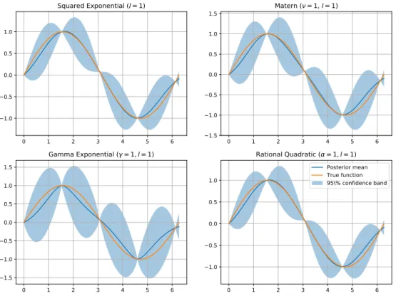
To demonstrate the behaviour of different acquisition functions on a step of Bayesian optimization, we will create a small script with our sine function example. This will help us understand visually the trade-off between exploration and exploitation in each case. The code provided in Appendix??produces Figure 3.1.

3.3.6

Why does Bayesian Optimization work?

In this small section, we will consider very briefly why the Bayesian Optimization procedure is efficiently making use of the information provided by the mean and variance posterior distribution of the GP. The explanation is mostly visual by means of Figure 3.2. The plot shows a Gaussian Process regression model, as well as its confidence interval, comprised from a lower confidence bound L = µ(x)−qσ(x) and an upper confidence boundU =µ(x) +qσ(x) for a quantileq >0.

In practice, when we are interested in doing hyperparameter search in machine-learning, the algo-rithms are very blunt, in the sense that the most common strategies explore the entire space, either exhaustively or randomly. The acquisition functions defined in this chapter before use information from the Gaussian Process prior to explore efficiently the space. The specifics of each acquisition function have already been discussed, specially their exploration/exploitation balance, but they all share some common logic.

(34)

3.3. ON ACQUISITION FUNCTIONS 33

Figure 3.1: Acquisition function behaviour for Expected Improvement, Probability of Improvement, GP-UCB (β=.5) and GP-UCB(β= 1.5) in the sine function example.

0 1 2 3 4 5 6 2 0 2 0 1 2 3 4 5 6 0.00 0.05 0.10 0.15 Expected improvement 0 1 2 3 4 5 6 0.0 0.2 0.4 Probability of Improvement 0 1 2 3 4 5 6 0.5 0.0 0.5 1.0 GP-UCB = . 5 0 1 2 3 4 5 6 0 1 GP-UCB = 1.5

(35)

34 CHAPTER 3. BAYESIAN OPTIMIZATION

Figure 3.2: A visual explanation on why Bayesian optimization is efficient at exploring the space. It ignores all the input space where the UCB is lower than the point with maximum LCB.

0 1 2 3 4 5 6 7 1.0 0.5 0.0 0.5 1.0 max LCB Posterior mean Lower confidence bound Upper confidence bound Discarded region

Bayesian Optimization is efficient because it ignores all the space where the predicted upper confi-dence bound is lower than the maximum value of the lower conficonfi-dence bound. It only uses the space that fulfills this criteria, according to the strategy selected by the chosen acquisition function. This remains a very reasonable assumption throughout the whole optimization procedure. In practice, the framework resembles a branch-and-bound type algorithm, but probabilistically. The procedure assumes that the true function will lie, with high probability 1−δwithin both lower and upper confidence bounds respectively. However, there is always the probability δ of the function not fulfilling this criteria, in which case the fit surrogate Gaussian Process will be updated with further evaluations. The code for generating this particular representation can be consulted in Appendix A.7.

While plenty of theoretical properties are known for bandit algorithms in general, only some have been established for Bayesian Optimization recently. In particular, for the Gaussian Process surrogate some consistency proofs exist [23] in the one dimensional case and in the multidimensional by the use of partitioning [16, 36]. Finite sample bounds have been provided recently for the GP-UCB acquisition function [33], while this was only proven for the fixed hyperparameter setting. However, despite the recent interest in theoretical properties of this framework, the gap between these and practice is still large [32].

3.4

Role of GP hyperparameters in optimization

We already considered the role of hyperparameters in Gaussian Process regression in section 2.5. However, one may wonder how the estimation of this parameters, one way or another may affect the optimization procedure. So far, we have assumed that during the optimization procedure, parameters θ were given.

(36)

3.5. OPTIMIZING THE ACQUISITION FUNCTION 35

Here we will consider two ways of handling hyperparameters during the optimization procedure, the one we presented, type II maximum likelihood estimation and approximate marginalization. For the moment, consider a generic acquisition function α:X ×Θ→_R, whereθ∈Θ are our Gaussian Process hyperparameters. Naturally, one wishes to marginalize the uncertainty caused by θ with the following expression:

α(x) =_Eθ_|D_n[α(x, θ)] =

Z

Θ

α(x|θ)p(θ|Dn)dθ. (3.15)

The simplest way to do this is what we saw in 2.37, to optimize the marginal log-likelihood to obtain MAP estimates ˆθMAP. Then, in each step of the optimization procedure, we simply maximize:

ˆ

α(x) =α(x,θˆ) (3.16)

That is, we optimize the acquisition function defined by theoptimalhyperparameters for the Gaussian Process determined in each step. Again, optimizing the marginal log-likelihood is a problem of its own, but it is common to use quasi-Newton methods such as L-BFGS-B methods.

A more Bayesian approach is to incorporate the uncertainty ofθinto our model, since it may have an important role in guiding exploration. Point estimates are in a sense winners that may not capture the complexity of the response surface. The second approach we will be considering here, will be therefore to marginalize out hyperparameters using Markov Chain Monte Carlo (MCMC) sampling techniques. In practice, we will need to averageM samplesnθ(ni)

oM i=1

from the posterior distributionp(θ|Dn):

Eθ|Dn[α(x, θ)]≈ 1 M M X i=1 α(x, θ_n(i)) (3.17)

Since it is not possible to have an analytical expression for the posterior distribution p(θ|Dn), it is

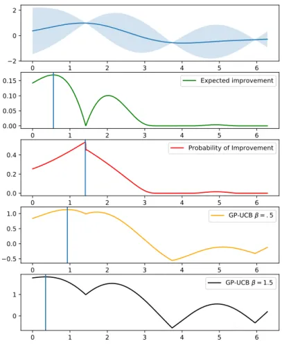
common to use MCMC techniques like Hamiltonian Monte Carlo [24] to produce a sequence of samples whose stationary distribution is the posterior we are looking for. OnceM valid samples are obtained, they are evaluated in the acquisition function and averaged. pyGPGO implements theseintegratedacquisition functions using the pyMC3 software [9]. A plot of sampled Gaussian Process associated with its posterior sampledp(θ|Dn) can be seen in Figure 3.3. Its associated script can be checked in Appendix A.6.

Quadrature methods can be used instead of MCMC techniques, yielding a weighted mixture:

Eθ|Dn[α(x, θ)]≈ M X i=1

ωiα(x, θ_n(i)) (3.18)

However, and to finish this section, in the problems that we will tackle in the experiments, it is usually a bad idea to estimate kernel hyperparameters. Estimating these hyperparameters with few function evaluations is a very challenging task, and can lead to disastrous results, as proven in [3, 8]. The marginal log-likelihood surface can easily fall into traps or be very flat, as seen by the (not cherry-picked) example in Figure 2.4. Even the more advanced MCMC or quadrature methods still suffer from this problem [38].

3.5

Optimizing the acquisition function

We have presented many acquisition functions in this chapter and provided a simple example to demon-strate basic functionality. However, so far, we have assumed that the acquisition function can be easily optimized. This is however, a problem of its own. The reader may be thinking that we have, in fact, changed one optimization problem (the one where we are interested in optimizing f) for another! (in which we now have to optimize α). This is technically true, but bear in mind that while f is very ex-pensive to evaluate, αis very cheap, and it is reasonable to spend a bit more computational effort in evaluatingαif it implies having to evaluatef less.

(37)

36 CHAPTER 3. BAYESIAN OPTIMIZATION

Figure 3.3: Means of 200 posterior predictive distributions, taken from associated GPs to each posterior samplep(θ|Dn) in the MCMC procedure. The integrated acquisition functions better take into account

the uncertainty of hyperparameters, which leads to less peaky functions.

0

1

2

3

4

5

6

1.0

0.5

0.0

0.5

1.0

Sampled data

0

1

2

3

4

5

6

0.00

0.01

0.02

(38)

3.6. COMPUTATIONAL COSTS 37

Maximizingα, however, is not an easy task. The acquisition function is often multi-modal and there-fore non-convex, as it can be see again in Figure 3.1. Theoretical convergence, furthermore, is only guaranteed when the optimal pointx∗ in the acquisition function is found [36]. At the end of the day, we encounter yet another global optimization problem that needs to be solved. From a practical point of view, there are many approaches the community has taken to solve this problem, from discretization [32] to adaptive-grids [2]. If gradient information is available (rarely the case), a multi-start gradient ascent approach can be taken [22]. Evolutionary approaches like CMA-ES can also be used [11]. pyGPGO, in the GPGO module uses by default a multi-start quasi-Newton method (L-BFGS-B) to optimize the acquisition function, which in practice seems to work reasonably well.

Other methods have been propo