Accepted Manuscript
Maximization of energy absorption for a wave energy converter using the deep machine learning
Liang Li, Zhiming Yuan, Yan Gao
PII: S0360-5442(18)31857-7
DOI: 10.1016/j.energy.2018.09.093
Reference: EGY 13787
To appear in: Energy
Received Date: 12 February 2018 Revised Date: 31 July 2018 Accepted Date: 13 September 2018
Please cite this article as: Li L, Yuan Z, Gao Y, Maximization of energy absorption for a wave energy converter using the deep machine learning, Energy (2018), doi: https://doi.org/10.1016/ j.energy.2018.09.093.
M
AN
US
CR
IP
T
AC
CE
PT
ED
Maximization of energy absorption for a wave energy converter using the
1
deep machine learning
2
Liang Li, Zhiming Yuan*, Yan Gao 3
Department of Naval Architecture, Ocean and Marine Engineering, University of Strathclyde, 100 Montrose Street, 4
Glasgow, G4 0LZ, UK 5
*
Corresponding author: [email protected]. 6
Abstract
7
A controller is usually used to maximize the energy absorption of wave energy converter. Despite the 8
development of various control strategies, the practical implementation of wave energy control is still 9
difficult since the control inputs are the future wave forces. In this work, the artificial intelligence 10
technique is adopted to tackle this problem. A multi-layer artificial neural network is developed and 11
trained by the deep machine learning algorithm to forecast the short-term wave forces. The model 12
predictive control strategy is used to implement real-time latching control action to a heaving point-13
absorber. Simulation results show that the average energy absorption is increased substantially with 14
the controller. Since the future wave forces are predicted, the controller is applicable to a full-scale 15
wave energy converter in practice. Further analysis indicates that the prediction error has a negative 16
effect on the control performance, leading to the reduction of energy absorption. 17
Keywords: wave energy converter; wave energy control; energy absorption; neural network; deep
18
machine learning; wave force prediction. 19
1.
Introduction
20
To keep up with the growth of global energy demand, various energy systems have been 21
developed to extract power from marine energy sources (offshore wind, ocean waves, tide, etc) [1-3]. 22
Compared with other marine energy resources, wave energy is a kind of resource with high power 23
density and all-day availability. Owing to these advantages, wave energy is regarded as a prospective 24
solution to the sustainable generation of power. The device used to harvest energy from ocean waves 25
is called the wave energy converter (WEC). Li et al. [4] showed the power output of an oscillating-26
body WEC installed on a spar-type floating wind turbine. He et al. [5] utilized a floater breakwater to 27
harvest energy from the waves. Experimental study of the concept was performed. Falcao and 28
Henriques [6] presented a review on the oscillating-water-column WEC. Stansby et al. [7] examined 29
the dynamics of multi-float WEC concept M4. 30
Although a set of WEC concepts have been developed, the energy harvesting efficiency is still not 31
satisfactory, especially in the off-resonance state. One of the solutions is the usage of a non-linear 32
power take-off (PTO) system. Zhang and Yang [8] showed that a PTO system with nonlinear spring 33
M
AN
US
CR
IP
T
AC
CE
PT
ED
oscillating-body WEC with three different PTO systems. They showed that the nonlinear behavior of 35
the PTO was beneficial to the power capture. An more widely accepted approach is to regulate the 36
WEC dynamics with a controller. Babarit et al. [10] studied how the declutching control influenced 37
the energy absorption of a WEC in regular and irregular waves. Tom et al. [11] optimized the power 38
capture of an oscillating surge WEC using the pseudo-spectral control method. The latching control 39
was firstly introduced by Budal and Falnes [12]. They found that one condition for maximizing 40
energy absorption was to keep the velocity in phase with the wave excitation force. Inspired by their 41
pioneering work, many researchers begin to adopt the latching control to enhance wave energy 42
efficiency. Babarit and Clement [13] assessed the benefits produced by the latching control. Based on 43
the pre-generated wave elevations, the optimal command theory was applied to derive the control 44
command. Henriques et al. [14] applied the latching control to an oscillating-water-column WEC. 45
Until now, the WEC control studies mainly concentrate on the development of control strategy 46
whereas the practical application of control is seldom reported. It is mainly because the 47
implementation of the controll to a realistic WEC requires the prediction of future wave forces. 48
Given the explosive growth of the artificial intelligence, the deep machine learning algorithm 49
based on the artificial neural network has been widely used for regression and classification. The 50
artificial neural network was firstly proposed by Mcculloch and Pitts [15]. At that time, the structure 51
of the neural network was very simple since the inference between densely connected nets with many 52
hidden layers is rather difficult. In 2006, Hinton et al. [16] proposed a fast, greedy algorithm for the 53
multi-layers network. Their work marked the era of ‘deep learning’. Although the deep machine 54
learning is basically employed in the recognition and interaction of signal, it is also powerful for 55
prediction in many fields. Lv et al. [17] used the deep learning approach to predict the traffic flow. 56
Islam and Morimoto [18] forecasted the inside air temperature of a pillar cooler with the neural 57
network. Recently, the machine learning was introduced to marine hydrodynamic prediction. 58
Pourzangbar et al. [19] predicted scour of breakwaters using the genetic programming and the 59
artificial neural network, respectively. Ebtehaj et al. [20] developed an integrated framework of 60
learning machines to predict scour at pile groups. 61
The present study is aimed at developing a real-time controller applicable in practice by 62
considering the short-term wave force forecasting. An artificial neural network is developed for the 63
wave force prediction. The neural network is trained with the deep machine learning algorithm to 64
learn the underlying relationship between wave forces in the past and future wave forces. The smart 65
controller is implemented to a heaving point-absorber to maximize the energy absorption. The 66
advantage of the neural network against traditional prediction method will be discussed. 67
2.
Numerical model
68
M
AN
US
CR
IP
T
AC
CE
PT
ED
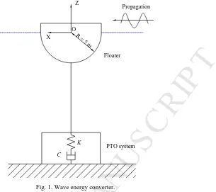
electrical power. The floater, a hemisphere with a radius of 5 m, is rigidly connected to the PTO 71
system fixed at the seabed. Only heave motion of the floater is allowed. 72
73
Fig. 1. Wave energy converter. 74
The generator force is modeled with a linear damping coefficient C and stiffness K. According to 75
Vicente et al. [21], the stiffness of a PTO system is typically around ten percent of the hydrostatic 76
coefficient. Therefore, K = 0.1ρgπR2 is adopted. ρ is the water density and g is the acceleration of
77
gravity. Fig. 2 illustrates the sensitivity of the PTO system to wave frequency ω and damping
78
coefficient C. To harvest as much energy as possible, C = 8.14×10⁵ kg/s is used. The controller 79
regulates the WEC response by locking and releasing the floater alternately following a certain rule. A 80
very large but finite damping coefficient c is used to lock the floater. This kind of control is widely 81
known as the latching control. 82
[image:4.595.191.496.111.382.2]83
Fig. 2. The sensitivity of energy absorption to wave frequency and damping coefficient C in regular waves. Wave amplitude 84
A = 1 m. 85
K
C
R = 5 m
PTO system Floater Z
X
O
Propagation
5.0E+05 1.0E+06 1.5E+06 2.0E+06 0.2
0.4 0.6 0.8 1.0 1.2 1.4
ω
(
ra
d
/s
)
C (kg/s)
0.000 1.050 2.100 3.150 4.200 5.250 6.300 7.350 8.400
M
AN
US
CR
IP
T
AC
CE
PT
ED
The linear potential flow theory is adopted to address the wave-structure interaction. The viscous 86
effect is not considered. It is worth noting that the linear dynamic model is invalid in extreme sea state, 87
where the free surface condition involves strong nonlinearity. Since a full-scale WEC just works in 88
moderate sea state, the linear dynamic model is still applicable. A right-handed coordinate system 89
fixed to the earth is used (see Fig. 1). The center of the coordinate system is fixed at the mean sea 90
surface. Z axial is positive upward. X axial is along the propagation direction of the sea waves. 91
Based on the impulse response theory [22], the time-domain motion equation of the floater is given 92
by 93
(
)
20
( ) ( ) ( ) ( ) ( ) ( ) ( ) ( ) ( )
t
wave
M +m z t&& +
∫
H t−τ τ τ ρ πz& d + g R z t =F t −Cz t& −Kz t −β t cz t& (1)94
where M is the mass of the floater and m is the added mass corresponding to infinite frequency. ,
95
and are the displacement, velocity and acceleration. Fwave is the wave excitation force. β(t) is the 96
binary control sequence. When β = 1, the floater is locked; when β = 0, it is free to oscillate. The 97
point-absorber switches abruptly between two states (β = 0,1) so that the latching control is a bang-98
bang control. H is the so-called retardation kernel function which represents the memory effect of 99
radiation force. It can be obtained either from the added mass a(ω) or the potential damping b(ω) 100
0 0
2 ( ) 2
( ) b sin( ) ( ) cos( )
H t ω ωt dω a ω ωt dω
π ω π
∞ ∞
=
∫
=∫
(2)101
Although Eq. (1) is widely used to simulate the wave-structure interaction, such form makes it 102
inconvenient to implement the control strategy. An alternative model is thus developed to simulate the 103
dynamics of the point-absorber in random waves, in which the convolution term is replaced by a state-104 space representation. 105 0 ( ) ( ) ( ) ( ) ( ) ( ) t
H t z d t
t t z t
τ τ τ
− =
= +
∫
& vv v
& & Cu
u Au B
(3) 106
where , and are constant matrices identifying the system with dimensions n×n, n×1 and 1×n. n 107
is the order of the system. These matrices can be derived from the hydrodynamic coefficients of the 108
point-absorber by system identification. u is an intermediate vector with dimension n×1. Define a 109
state vector x = [ , , ] with dimension (n+2)×1. Then Eq. (1) can be re-expressed as 110
2
0 1 0
, wave
g R K C c F
M m M m M m M m
ρ π β
= ⋅ + + + = − − − = + + + + 0 0 0 & v v v x x C B A γ η γ η γ η γ η γ η γ η γ η
γ η (4)
111
Eq. (4) is a first-order, one-variable differential formula, which is easier to handle. Given the initial 112
M
AN
US
CR
IP
T
AC
CE
PT
ED
movement can be obtained by the 4th Runge-Kutta method. Then, the average energy absorption 114
during simulation interval [0, T] is given by 115 2 0 1 ( , ) T
P C z t dt
T
β
=
∫
⋅& (5)116
The random sea waves can be efficiently approximated by a set of regular wave components with 117
various frequencies and random phases 118
( )
1
( ) Re
2 ( )
j j N i t j j j j
t A e
A S ω ε ξ ω ω + = = =
∑
(6) 119where Aj, ωj, and εj are the amplitude, frequency and random phase of the regular wave component j. 120
S(ω) is the wave spectrum adopted to describe the statistical feature of the random waves. N is the 121
number of regular wave components in the wave spectrum. If ωj is uniformly distributed over the 122
wave frequency range, the stochastic wave elevations will start to repeat after a certain duration [23]. 123
To address this issue, the correction technique in Ref [24] is adopted here. The wave frequency range 124
is first uniformly divided into N segments and ωj is afterward randomly distributed within segment j. 125
Given the time series of random wave elevations, the linear wave forces are obtained with the first-126
order transfer function Ψ. 127
( )
1
( ) Re ( ) j j
N
i t
wave j j
j
F t ψ ω A e ω ε+
=
=
∑
(7)128
3.
Control strategy
129
3.1.
Optimal command theory
130
The objective of latching control is to maximize the average energy absorption through the binary 131
control sequence β(t) 132
2
0
1
max ( , )
T
P C z t dt
T
β
=
∫
⋅& (8)133
From a mathematical point of view, it is required to find the maximum of P subject to constraint 134
Eq. (4). If the incident wave is regular, it becomes an impedance matching problem and can be solved 135
analytically [13]. Otherwise, the solution is non-causal [25]. Regardless of the incident waves, define 136
a Hamiltonian H: 137
2
( )
H =Cz& +λ γλ γλ γλ γ ⋅ +x ηηηη (9)
138
λ is a state vector with dimension 1×(n+2), which can be regarded as the Lagrange multipliers. γ and η 139
have the same definitions in Eq. (4). 140
According to the Pontryagin’s maximum principle, the optimal β is the one maximizing the 141
Hamiltonian at every time instant throughout [0, T]. The Hamiltonian is a linear function of β so that β
M
AN
US
CR
IP
T
AC
CE
PT
ED
must be the extremal values (0 or 1) to maximize the Hamiltonian. It is easy to find that the 143
Hamiltonian reaches the maximum value on condition that 144
2
1 0
0
cz otherwise
λ
β
= <
&
(10) 145
Assume that the random waves within the interval [0, T] are already known, the time series of 146
floater movement can be calculated. Subsequently, it is required to calculate at each time instant
147
and apply the latching control based on the binary sequence. Please note that the sate vector satisfies 148
the following relationships. 149
( , , ), 1,2,..., 2
( )
i i
H
t i n
x
T
λ
= −∂β
= +∂ =0
&
x
λλλλ
(11) 150
Eq. (11) cannot be solved numerically like an initial value problem as the final condition is given 151
here. In Ref [26], the canonical equations were solved based on the combination of discretization and 152
dynamic programming. Zhong and Yeung [27] derived the control sequence with the so-called 153
quadratic programming formulation. In our study, an iterative process is applied to calculate λ. Firstly, 154
run the simulation with β(t) = 0 to obtain the motions free of latching action by integrating Eq. (4) 155
forward from t = 0 to t = T. Subsequently, determine λ by integrating Eq. (11) backwards from t = T to 156
t = 0 (λ(T) = 0 is now an initial condition). Based on Eq. (10), the control sequence β(t) is derived. 157
Iterate the process with the updated control sequence until it converges. 158
3.2.
Real-time control
159
The optimal command theory cannot be applied directly since it is impossible to know the wave 160
forces over the entire interval. Nevertheless, one can forecast the short-term wave forces over a 161
relatively short interval [t, t+∆t] so that the optimal command theory can be used within the prediction
162
interval. It is the basic idea of the real-time control strategy in this study. 163
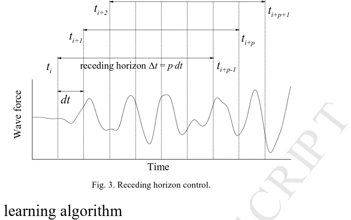
Assuming that a wave force prediction model has been developed (the prediction model is the 164
neural network in the present study), the procedure of the real-time control is illustrated in Fig. 3. At 165
time instant ti, collect the historical wave forces and perform the forecasting within [ti+1, ti+1+∆t]. Then, 166
the control sequence β(t), t ∈ [ ti+1, ti+1+∆t] can be estimated with the optimal command theory. Please 167
note that only the predicted control sequence β(ti+1) is adopted. At time instant ti+1, apply the control 168
action which has been predicted at the previous step and repeat the process again to predict the control 169
action at time instant ti+2. By repeating this algorithm step by step, the real-time control is 170
implemented throughout the entire interval. Such a real-time control is also known as the receding 171
horizon control or the model predictive control. Since the energy absorption is maximized over the 172
M
AN
US
CR
IP
T
AC
CE
PT
ED
174
Fig. 3. Receding horizon control. 175
4.
Machine learning algorithm
176
The machine learning algorithm is a member of the broad family of artificial intelligence. Its 177
fundamental architecture is the artificial neural network, which is inspired by the biological neural 178
network. The main idea of using machine learning to predict wave forces is that the neural network 179
can learn and recognize the underlying relationships between the wave forces in the past and the 180
coming wave forces through sufficient training examples. 181
4.1.
Neural network
182
Fig. 4 illustrates the structure of an artificial neural network, which is composed of the input layer, 183
the hidden layers, and the output layer. For the problem in this study, the input is namely the recorded 184
wave forces in the past and the output is the prediction of wave forces over the predictive horizon. 185
Several neurons are located in the layers to process the input signals. Two sets of parameters, weight 186
w = (w11, w12,…, wji,…) and threshold b = (b11, b12,…, bij,…) are used to value the importance of the 187
input signal. wji and bji are the parameters of the i-th neuron at the j-th layer. The estimated signal is 188
subsequently normalized by the activation function before transferring to the next layer. The sigmoid 189
function (σ(x) = 1/(1+e-x)) is selected here as the activation function. 190
[image:8.595.146.498.75.296.2]191
Fig. 4. Illustration of signal transformation between layers. 192
ti+p+1
ti+2
ti+p
ti+1
ti+p-1
ti
dt
W
av
e
fo
rc
e
Time
M
AN
US
CR
IP
T
AC
CE
PT
ED
4.2.
Training algorithm
193
Before the neural network can be used for prediction, one has to tune the parameters w and b make 194
it compatible with the problem concerned. This is fulfilled by training the network with a large 195
number of examples (big data) so that it can learn how to predict the wave forces according to 196
previous ‘experiences’. A cost function Θ is introduced to estimate the performance of the neural
197
network. 198
2 1
1 ( , )
2 L
k k
k
y a
L =
Θ w b =
∑
− (12)199
L is the number of training examples. yk and ak are the prediction output and the prediction target 200
corresponding to the k-th training example. Given the examples, the objective of ‘training’ is to find 201
the optimal parameters w and b, which minimize the cost function Θ. The optimal values are searched
202
using the gradient descent method. 203
'
'
ji ji
ji
ji ji
ji
w w
w
b b
b
κ
κ
∂Θ = −
∂ ∂Θ = −
∂
(13) 204
wji' and bji' are the updated weight and threshold after training. is the so-called learning rate, 205
representing the sensitivity of the network to training example. In the case of = 0, the network learns 206
nothing from the training examples. Now, the key point is to acquire the gradient of cost function Θ at
207
various layers. The backpropagation algorithm is used here to estimate the gradient of cost function. 208
Start the backpropagation process by estimating the gradient at the output layer. Then the gradient at 209
previous layers can be estimated. Continue the backpropagation algorithm until the gradients at all 210
layer are obtained. Eventually, update parameters w and b with the acquired gradients. 211
We demonstrate the procedure of the training process with a simple case. Assume that the network 212
has two hidden layers and each layer has only one neuron (see Fig. 4). The neural network is trained 213
with a single example (L = 1). Denote y0 the input to the network, the output of hidden layers is given
214
by y1 = σ(w1y0+b1) and y2 = σ(w2y1+b2). The final output of the network is y3 = w3y2+b3. Then, the
215
deviation of cost function at the output layer is given by 216
3 2 1 2
3
'(w y b )
y
δ = ∂Θ⋅σ +
∂ (14)
217
The deviation of cost function at the hidden layer is obtained with the backpropagation algorithm 218
1 1 ( 1 )
i wi i w yi i bi
δ = +δ σ+ − + , i = 1,2 (15)
219
At this point, the deviation of cost function at all layers are acquired. Afterward, the gradient of 220
M
AN
US
CR
IP
T
AC
CE
PT
ED
1 i i
i i
i
b
y w
δ
δ
−
∂Θ = ∂
∂Θ = ∂
, i = 1,2,3 (16)
222
With the gradient of cost function, the weights and thresholds are updated on the basis of Eq. (13). 223
Iterate the above process until the pre-defined termination criteria are satisfied. Please refer to [28] for 224
detailed procedures of the training process for more general cases. 225
4.3.
Estimation of prediction performance
226It is well-known the that successful implementation of real-time control requires accurate 227
prediction of wave forces. Otherwise, the control performance may become bad [29]. The prediction 228
ability of the trained neural network is checked through comparison with the traditional prediction 229
methodology-grey model GM(1,1). The detailed procedure of using the grey model for prediction can 230
be found in Appendix A. The random wave elevations measured in the Ref [30] is used to examine 231
the prediction ability of the two models. The measured data were low-pass filtered to remove the 232
high-frequency wave noise. The significant wave height of the random wave elevations is 0.04 m and 233
the wave peak period is 1.13 s. Although the neural network forecasts wave forces in the present 234
research, it can be validated by the wave elevations since both variables are random signals by nature. 235
We select 100 s of wave elevation measurement. The first 50 s data are used to train the neural 236
network and the last 50 s are used for validation. Hong and Billings [31] proposed a simplified 237
prediction index for quantitative assessment of the prediction 238
2 0 2 0
( ) ( )
( )
T
T
h d
Er t
h t d
τ τ
τ τ τ
∆ =
+ ∆
∫
∫
(17)239
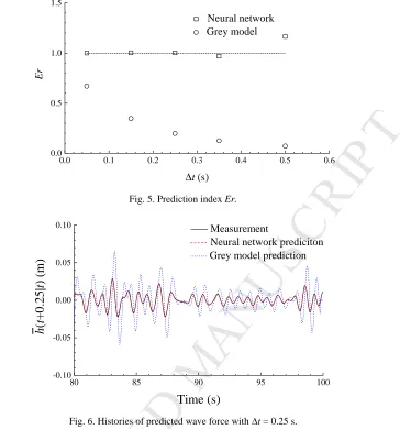
where h(t) is the measured wave elevation at time instant t; h t( + ∆t t) is the ∆t time ahead wave
240
elevation predicted at time instant t. Er < 1 indicates that the predicted values are larger than the target 241
and vice versa. Er close to 1 represents a good prediction capacity. 242
Fig. 5 compares the prediction performances of the two models. The neural network behaves better 243
than the grey model. The index Er estimated by the neural network is generally around 1. Fig. 7 plots 244
the predicted wave force histories. The force predicted by the neural network agrees well with the 245
M
AN
US
CR
IP
T
AC
CE
PT
ED
[image:11.595.131.495.78.468.2]247
Fig. 5. Prediction index Er. 248
249
Fig. 6. Histories of predicted wave force with ∆t = 0.25 s. 250
5.
Validation
251
Two aspects of validation are performed, namely the WEC dynamics and the control sequence 252
derivation. 253
5.1.
WEC dynamics
254
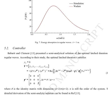
Firstly, we validate the dynamic model in the absence of the latching control. The energy 255
absorption in a set of unit regular waves with various oscillation frequencies is simulated. The results 256
are compared with those estimated by frequency-domain hydrodynamic analysis programme Wadam 257
[32]. Please note that the point-absorber is a linear system without the latching control so that Wadam 258
is applicable here. The PTO system force is modeled with the ‘additional damping’ and ‘additional 259
stiffness’ options provided in Wadam. As displayed in Fig. 7, the agreement between the two 260
simulation tools are very good. 261
0.0 0.1 0.2 0.3 0.4 0.5 0.6
0.0 0.5 1.0 1.5
E
r
∆t (s)
Neural network Grey model
80 85 90 95 100
-0.10 -0.05 0.00 0.05 0.10
h
(t
+
0
.2
5
|
t)
(
m
)
Time (s)
Measurement
M
AN
US
CR
IP
T
AC
CE
PT
ED
[image:12.595.54.513.78.484.2]262
Fig. 7. Energy absorption in regular waves. A = 1 m. 263
5.2.
Controller
264
Babarit and Clement [13] presented a semi-analytical solution of the optimal latched duration in 265
regular waves. According to their study, the optimal latched duration t satisfies 266
[
]
{
}
2
1 2 1 2
' 1 1 ( )
0
, , , ,
( ) ( ) Re ( )( )
0 0 0
' 0 0 0 , /
0 0
n n
t i i t
y
y y y y
e e e e i e
t t
A
ω ω ω ε
π ω
+ +
∆ − ∆ ∆ − +
= =
= − + ⋅ × − − ×
= ∆ = −
K
v Y
I γγγγ γγγγ I γγγγ I γ ηγ ηγ ηγ η
γγγγ
(18) 267
where I is the identity matrix with dimension (n+2)×(n+2). n is still the order of the system. The 268
detailed derivation of the semi-analytic solution can be found in Ref [13]. 269
The latched duration suggested by Eq. (18) and simulated by the present controller are compared 270
in Fig. 8. As shown, the optimal latched duration increases with the wave period, implying that a 271
stronger latching action is needed in the case of long waves to regulate the response. Some 272
discrepancies are observed because the absolute latching control (locking the WEC instantaneously) 273
was used in Ref [13] whereas the present simulation applies a large damping force to lock the floater. 274
0.0 0.5 1.0 1.5 2.0
0 20 40 60 80 100
P
(
k
W
)
ω (rad/s)
M
AN
US
CR
IP
T
AC
CE
PT
ED
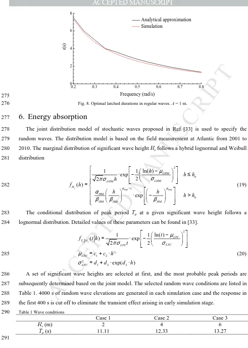
275Fig. 8. Optimal latched durations in regular waves. A = 1 m. 276
6.
Energy absorption
277
The joint distribution model of stochastic waves proposed in Ref [33] is used to specify the 278
random waves. The distribution model is based on the field measurement at Atlantic from 2001 to 279
2010. The marginal distribution of significant wave height Hs follows a hybrid lognormal and Weibull 280 distribution 281 2 0 1 0
1 1 ln( )
exp 2 2 ( ) exp s HM HM LHM LHM LHM H HM
HM HM HM
h h h h f h h h h h α α µ σ πσ α
β β β
− − ⋅ − ≤ =
⋅ − >
(19) 282
The conditional distribution of peak period Tp at a given significant wave height follows a 283
lognormal distribution. Detailed values of these parameters can be found in [33]. 284
3
2
1 2 2
1 2 3
1 1 ln( )
( ) exp
2 2 exp( ) p s LTC T H LTC LTC c LTC LTC t
f t h
t
c c h
d d d h
µ σ πσ µ σ − = ⋅ − = + ⋅ = + ⋅ ⋅ (20) 285
A set of significant wave heights are selected at first, and the most probable peak periods are 286
subsequently determined based on the joint model. The selected random wave conditions are listed in 287
Table 1. 4000 s of random wave elevations are generated in each simulation case and the response in 288
[image:13.595.66.503.86.360.2]the first 400 s is cut off to eliminate the transient effect arising in early simulation stage. 289
Table 1 Wave conditions 290
Case 1 Case 2 Case 3
Hs (m) 2 4 6
Tp (s) 11.11 12.33 13.27
291
0.2 0.3 0.4 0.5 0.6 0.7 0.8
M
AN
US
CR
IP
T
AC
CE
PT
ED
6.1.
Regular waves
292
We first investigate the energy absorption in regular waves. Since the waves are regular, the wave 293
forces over the predictive horizon are given rather than predicted here. The predictive horizon is set to 294
0.2∙(2π/ω). The wave amplitude A is 1 m. Fig. 9 plots the sensitivity of energy absorption to wave
295
oscillation frequency. The control effect on the energy absorption is noticeable, especially within the 296
low-frequency range. 297
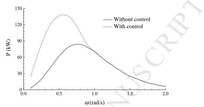
[image:14.595.150.496.184.366.2]298
Fig. 9. Average energy absorption in regular waves. A = 1 m. 299
Fig. 10 displays the phase portrait of the responses. It is obvious that the velocity phase is 300
regulated by the controller. The latching control is a kind of phase control by nature and it maximizes 301
energy absorption by tuning velocity phase. Fig. 11 displays the controlled motion and its relative 302
phase with respect to the wave forces. According to the velocity time-series, the point-absorber is 303
latched and released alternately so that the response is a succession of locked and ramp stages. Due to 304
the regulation of the controller, the velocity and the wave forces are in phase so that the wave forces 305
will always accelerate the floater and the floater carries more kinetic energy as a result. This property 306
has been widely used as the criterion to validate latching control since the work of Budal and Falnes 307
[12]. Therefore, Fig. 11 can be used to validate the present numerical model as well. 308
[image:14.595.36.513.359.741.2]309
Fig. 10 Phase portrait in regular wave. A = 1 m, ω = 0.5 rad/s. 310
0.0 0.5 1.0 1.5 2.0
0 30 60 90 120 150
P
(
k
W
)
ω (rad/s)
Without control With control
-1.5 -1.0 -0.5 0.0 0.5 1.0 1.5
-1.5 -1.0 -0.5 0.0 0.5 1.0 1.5
V
el
o
ci
ty
(
m
/s
)
Displacement (m)
M
AN
US
CR
IP
T
AC
CE
PT
ED
[image:15.595.165.496.76.266.2]311
Fig. 11. Responses of the floater in regular wave. A = 1 m, ω = 0.5 rad/s. 312
Nevertheless, it seems that the controller is not effective at all within the high-frequency range. 313
According to Fig. 8, the optimal latched duration reduces gradually when the wave frequency 314
increases and reduces to nearly zero in the case of very high-frequency waves. It implies that it is 315
unnecessary to regulate the point-absorber in high-frequency wave and thereby the energy absorption 316
is hardly increased. As pointed out in Ref [34], the optimal duration of a single locked stage is close to 317
half of the natural period of the WEC on condition that the PTO damping coefficient C is sufficiently 318
small (weak damping). Therefore, the solution of the control sequence is only available when the 319
wave period is sufficiently long. Although the damping coefficient C is very large in our model and 320
the sub-optimal receding horizon control is used here, this property can still help to interpret why the 321
latching control is merely effective in low-frequency waves. 322
6.2.
Irregular waves
323
In the real oceans, the waves are random and oscillate with multiple frequencies so that the wave 324
forces are unknown. To examine the validity of the smart controller, we run simulations in regular 325
waves where the short-term future wave forces are predicted by the neural network. Fig. 12 plots the 326
histories of floater velocity and wave forces. Like regular wave case, the point-absorber is also locked 327
frequently in random waves. Whenever the wave force and the velocity are reverse, the floater is 328
locked to avoid the slowing down of velocity. Once the floater is released, the velocity builds up 329
rapidly in a short time. Owing to the regulation of the controller, the velocity is generally in phase 330
with the wave forces. 331
20 30 40 50 60 70 80 90 100
-1.5 -1.0 -0.5 0.0 0.5 1.0 1.5 2.0
Velocity (without control) Velocity (with control) Wave force
Time (s)
V
el
o
ci
ty
(
m
/s
)
-800 -400 0 400 800 1200
W
av
e
fo
rc
e
(k
N
M
AN
US
CR
IP
T
AC
CE
PT
ED
332
Fig. 12. Responses of the point-absorber, Case1. 333
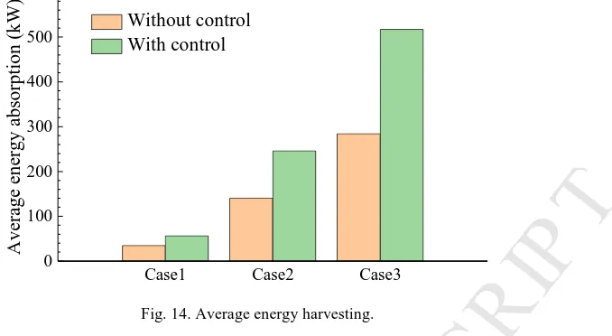
The control effect on the energy absorption is illustrated in Fig. 13. Although the point-absorber is 334
locked frequently, and the PTO systems stop working during the locked duration, the energy 335
extraction ramps once the point-absorber is set free since the velocity runs up rapidly during the ramp 336
stage. It leads to the enhancement of the average energy absorption. The 1-hr average energy 337
harvesting under various wave conditions is presented in Fig. 14. Generally, the point-absorber 338
produces 60%~80% more electrical energy with the smart controller. It manifests that the neural 339
network can be successfully applied in the real-time control of WEC. 340
341
Fig. 13. Power capture, Case1. 342
1000 1020 1040 1060 1080 1100
-1000 -500 0 500 1000
1500 Wave force
Velocity (Without control) Velocity (With control)
Time (s)
W
av
e
fo
rc
e
(k
N
)
-2.0 -1.5 -1.0 -0.5 0.0 0.5 1.0 1.5 2.0
V
el
o
ci
ty
(
m
/s
)
10000 1020 1040 1060 1080 1100
300 600 900 1200 1500
P
(k
W
)
Time (s)
M
AN
US
CR
IP
T
AC
CE
PT
ED
343
Fig. 14. Average energy harvesting. 344
As discussed in Section 3.2, the model predictive control can be regarded as a kind of sub-optimal 345
control. Consequently, the efficiency of the controller is evaluated by comparing with the optimal one. 346
Please note that by implementing the optimal control it inherently implies that the wave forces over 347
the entire interval are already known. Fig. 15 displays the control sequence using the two control 348
schemes. The control sequence predicted by the neural network is close to the optimal one, indicating 349
that the prediction accuracy of the neural network is satisfactory. Some discrepancies are observed 350
since the prediction deviation is unavoidable. Also, the model predictive control is sub-optimal by 351
nature and it cannot acquire the optimal sequence even in the absence of prediction deviation. 352
353
Fig. 15. Control sequence, Case 1. 354
Table 2 lists the average energy absorption obtained using the model predictive control and the 355
optimal control. Generally, the model predictive control underestimates the energy harvesting by no 356
more than 9%. Although the real-time control is sub-optimal, the control efficiency is still satisfactory 357
[image:17.595.155.494.85.271.2]even if the wave forces are predicted. 358
Table 2 Average energy absorption estimated by real-time control and optimal control. 359
Real-time control Optimal control
Case1 56 kW 61 kW
Case1 Case2 Case3 0
100 200 300 400 500 600
A
v
er
ag
e
en
er
g
y
a
b
so
rp
ti
o
n
(
k
W
)
Without control With control
1000 1020 1040 1060 1080 1100
0 1
β
Time (s)
M
AN
US
CR
IP
T
AC
CE
PT
ED
360
6.3.
Energy absorption with different prediction models
361
To demonstrate the advantage of the neural network against traditional prediction approach, the 362
neural network is compared with the grey model GM(1,1). The control efficiency will be evaluated to 363
show the accuracy of the two prediction models. 364
Table 3 lists the average power extraction of the point-absorber using different wave force 365
prediction models. As shown, the control efficiency is reduced substantially if the wave forces are 366
predicted by the grey model. Since the point-absorber is subject to identical wave forces, the 367
discrepancies on the control performance are completely caused by the prediction error. It thus 368
implies that the neural network is a more reliable prediction approach. 369
Table 3 Average power extraction with different prediction models 370
Case1 Case2 Case3
Neural network 56 kW 246 kW 517 kW
GM (1,1) 50 kW 201 kW 429 kW
371
Fig. 16 plots the optimal control sequence and the predicted sequence with respect to the two 372
prediction models. Due to the unavoidable prediction deviation, the predicted control sequence is 373
somewhat different from the optimal one. Nevertheless, it is easy to find that the sequence predicted 374
by the neural network is closer to the optimal one, attributing to the better prediction capacity. A more 375
appropriate control sequence indicates the point-absorber will be released and locked at the right time 376
M
AN
US
CR
IP
T
AC
CE
PT
ED
378
Fig. 16. Control sequence forecasted by different prediction models, Case1. (a) Optimal; (b) Neural network; (c) GM(1,1). 379
7.
Conclusions
380
Wave force prediction is necessary for the implementation of WEC real-time control. As proved in 381
previous studies, the prediction deviation will reduce the efficiency of real-time control and thereby 382
an accurate wave force prediction method is essential. In our work, an artificial neural network is 383
developed to predict the short-term wave forces. Based on the developed neural network, the real-time 384
latching control is implemented to a heaving point-absorber to maximize the energy extraction in 385
random waves. 386
The neural network is trained using the machine learning algorithm. The training process is based 387
on the backpropagation algorithm, in which the gradient of cost function at various layers are 388
estimated to update the weights and the thresholds. Based on a large number of training examples, the 389
weights and thresholds identifying the neural network are optimized gradually until the outputs agree 390
well the desired targets. 391
The point-absorber harvests more power with the real-time control, which is attributed to the 392
1000 1020 1040 1060 1080 1100
0 1
β
Time (s)
1000 1020 1040 1060 1080 1100
0 1
β
Time (s)
1000 1020 1040 1060 1080 1100
0 1
β
Time (s)
a
b
M
AN
US
CR
IP
T
AC
CE
PT
ED
alternately so that the velocity and the wave forces are in phase. In that case, the wave forces always 394
accelerate the point-absorber and the floater carries more kinetic energy. For the random wave 395
conditions considered in this study, the energy absorption is increased by 60%~80% with the smart 396
controller. Owing to the good prediction capacity of the neural network, the control efficiency is 397
satisfactory, just slightly lower than the optimal level. 398
Acknowledgment
399
This work is supported by China Scholarship Council [Grant No. 201506230127]. The authors are 400
grateful for their financial support. 401
References
402
[1] Bahaj AS, Batten WMJ, McCann G. Experimental verifications of numerical predictions for the 403
hydrodynamic performance of horizontal axis marine current turbines. Renew Energ. 404
2007;32(15):2479-90. 405
[2] Li L, Gao Y, Hu Z, Yuan Z, Day S, Li H. Model test research of a semisubmersible floating wind 406
turbine with an improved deficient thrust force correction approach. Renew Energ. 2018;119:95-105. 407
[3] Muliawan MJ, Karimirad M, Moan T. Dynamic response and power performance of a combined 408
Spar-type floating wind turbine and coaxial floating wave energy converter. Renew Energ. 409
2013;50:47-57. 410
[4] Li L, Gao Y, Yuan ZM, Day S, Hu ZQ. Dynamic response and power production of a floating 411
integrated wind, wave and tidal energy system. Renew Energ. 2018;116:412-22. 412
[5] He F, Huang ZH, Law AWK. An experimental study of a floating breakwater with asymmetric 413
pneumatic chambers for wave energy extraction. Appl Energ. 2013;106:222-31. 414
[6] Falcao AFO, Henriques JCC. Oscillating-water-column wave energy converters and air turbines: 415
A review. Renew Energ. 2016;85:1391-424. 416
[7] Stansby P, Moreno EC, Stallard T. Large capacity multi-float configurations for the wave energy 417
converter M4 using a time-domain linear diffraction model. Appl Ocean Res. 2017;68:53-64. 418
[8] Zhang XT, Yang JM. Power capture performance of an oscillating-body WEC with nonlinear snap 419
through PTO systems in irregular waves. Appl Ocean Res. 2015;52:261-73. 420
[9] Xiao XL, Xiao LF, Peng T. Comparative study on power capture performance of oscillating-body 421
wave energy converters with three novel power take-off systems. Renew Energ. 2017;103:94-105. 422
[10] Babarit A, Guglielmi M, Clement AH. Declutching control of a wave energy converter. Ocean 423
Eng. 2009;36(12-13):1015-24. 424
[11] Tom NM, Yu YH, Wright AD, Lawson MJ. Pseudo-spectral control of a novel oscillating surge 425
wave energy converter in regular waves for power optimization including load reduction. Ocean Eng. 426
M
AN
US
CR
IP
T
AC
CE
PT
ED
[12] Budal K, Falnes J. Interacting point absorbers with controlled motion, in Power from Sea Waves: 428
BM Count, Academic Press, 1980. 429
[13] Babarit A, Clement AH. Optimal latching control of a wave energy device in regular and 430
irregular waves. Appl Ocean Res. 2006;28(2):77-91. 431
[14] Henriques JCC, Gato LMC, Falcao AFO, Robles E, Fay FX. Latching control of a floating 432
oscillating-water-column wave energy converter. Renew Energ. 2016;90:229-41. 433
[15] Mcculloch WS, Pitts W. A Logical Calculus of the Ideas Immanent in Nervous Activity. B Math 434
Biol. 1943;5(4):115-33. 435
[16] Hinton GE, Osindero S, Teh YW. A fast learning algorithm for deep belief nets. Neural Comput. 436
2006;18(7):1527-54. 437
[17] Lv YS, Duan YJ, Kang WW, Li ZX, Wang FY. Traffic Flow Prediction With Big Data: A Deep 438
Learning Approach. Ieee T Intell Transp. 2015;16(2):865-73. 439
[18] Islam MP, Morimoto T. Non-linear autoregressive neural network approach for inside air 440
temperature prediction of a pillar cooler. Int J Green Energy. 2017;14(2):141-9. 441
[19] Pourzangbar A, Losada MA, Saber A, Ahari LR, Larroude P, Vaezi M, et al. Prediction of non-442
breaking wave induced scour depth at the trunk section of breakwaters using Genetic Programming 443
and Artificial Neural Networks. Coast Eng. 2017;121:107-18. 444
[20] Ebtehaj I, Bonakdari H, Moradi F, Gharabaghi B, Khozani ZS. An integrated framework of 445
Extreme Learning Machines for predicting scour at pile groups in clear water condition. Coast Eng. 446
2018;135:1-15. 447
[21] Vicente PC, Falcao AFO, Justino PAP. Nonlinear dynamics of a tightly moored point-absorber 448
wave energy converter. Ocean Eng. 2013;59:20-36. 449
[22] Cummins W. The impulse response function and ship motions. Washington DC: David Taylor 450
Model Basin; 1962. p. 101-9. 451
[23] Faltinsen OM. Sea Loads on Ships and Offshore Structures: Cambridge University Press, 1993. 452
[24] Li L, Hu ZQ, Wang J, Ma Y. Development and Validation of an Aero-hydro Simulation Code for 453
Offshore Floating Wind Turbine. J Ocean Wind Energy. 2015;2(1):1-11. 454
[25] Falnes J. Ocean waves and oscillating systems: linear interactions including wave-energy 455
extraction: Cambridge university press, 2002. 456
[26] Li G, Weiss G, Mueller M, Townley S, Belmont MR. Wave energy converter control by wave 457
prediction and dynamic programming. Renew Energ. 2012;48:392-403. 458
[27] Zhong Q, Yeung RW. An Efficient Convex Formulation for Model-Predictive Control on Wave-459
Energy Converters. Conference An Efficient Convex Formulation for Model-Predictive Control on 460
Wave-Energy Converters. American Society of Mechanical Engineers, p. V010T09A35-VT09A35. 461
[28] Nielsen M. Neural Networks and Deep Learning2017. 462
M
AN
US
CR
IP
T
AC
CE
PT
ED
[30] Li L, Gao Y, Hu ZQ, Yuan ZM, Day S, Li HR. Model test research of a semisubmersible floating 465
wind turbine with an improved deficient thrust force correction approach. Renew Energ. 2018;119:95-466
105. 467
[31] Hong X, Billings S. Time series multistep‐ahead predictability estimation and ranking. Journal of 468
Forecasting. 1999;18(2):139-49. 469
[32] Veritas DN. WADAM—Wave Analysis by Diffraction and Morison Theory. SESAM user’s 470
manual, Høvik1994. 471
[33] Li L, Gao Z, Moan T. Joint Distribution of Environmental Condition at Five European Offshore 472
Sites for Design of Combined Wind and Wave Energy Devices. J Offshore Mech Arct. 473
2015;137(3):031901. 474
[34] Babarit A, Duclos G, Clement AH. Comparison of latching control strategies for a heaving wave 475
energy device in random sea. Appl Ocean Res. 2004;26(5):227-38. 476
477
M
AN
US
CR
IP
T
AC
CE
PT
ED
、 479Appendix A
480Step1: At time instant ti, collect the raw data X over the past few seconds 481
(
x1,x2, ...,xn)
=
X (A.1)
482
Step2: Generate an accumulated series Y 483
(
1 2)
1 , ,..., , 1,2,..., n k k i i
y y y
y x k n
= = =
∑
= Y (A.2) 484Step3: Generate the so-called background series Z 485
(
)
(
2 3 1)
, ,...,
/ 2
n
k k k
z z z
z y y −
= = +
Z
(A.3) 486
Step4: Set the grey differential formula 487
, 2, 3,..,
k k
x +az =b k= n (A.4)
488
Step5: Estimate parameters a and b with the least square method 489
( )
12 2 3 3 1 1 , 1 T T n n a b z x z x z x − = − − = = −
M M M
A A A B
A B
(A.5) 490
Step6: Establish the first order-one variable grey model GM(1,1) to predict the random signal 491
within interval [ti+1, ti+p] 492
( ) 1
1 1
ˆ ˆ ˆ
ˆ
n p n p n p
a n p n p
x y y
b b
y y e
a a + + + − − + − + = − = − + (A.6) 493
M
AN
US
CR
IP
T
AC
CE
PT
ED
A smart real-time controller is developed.
The smart controller uses artificial neural network to predict short-term wave forces.
The neural network is trained by the deep learning algorithm.
The prediction accuracy of the neural network is satisfactory.