Multi agent collaborative search based on Tchebycheff decomposition

(will be inserted by the editor)

Multi Agent Collaborative Search Based on Tchebycheff

Decomposition

Federico Zuiani · Massimiliano Vasile

Received: date / Accepted: date

Abstract This paper presents a novel formulation of Multi Agent Collaborative Search, for multi-objective optimization, based on Tchebycheff decomposition. A population of agents combines heuristics that aim at exploring the search space both globally (social moves) and in a neighborhood of each agent (individualistic moves). In this novel formulation the selection process is based on a combination of Tchebycheff scalarization and Pareto dominance. Furthermore, while in the previous implementa-tion, social actions were applied to the whole population of agents and individualistic actions only to an elite subpopulation, in this novel formulation this mechanism is inverted. The novel agent-based algorithm is tested at first on a standard benchmark of difficult problems and then on two specific problems in space trajectory design. Its performance is compared against a number of state-of-the-art multi-objective op-timization algorithms. The results demonstrate that this novel agent-based search has better performance with respect to its predecessor in a number of cases and con-verges better than the other state-of-the-art algorithms with a better spreading of the solutions.

Keywords agent-based optimization· multi-objective optimization· memetic strategies

F. Zuiani

School of Engineering, University of Glasgow, Glasgow, UK Tel.: +44(0)141 548 4558

Fax: +44(0)141 552 5105

E-mail: [email protected]

M. Vasile

Department of Mechanical & Aerospace Engineering, University of Strathclyde, Glasgow, UK Tel.: +44(0)141 548 2083

Fax: +44(0)141 552 5105

1 Introduction

Multi-Agent Collaborative Search (MACS) has been proposed as a framework for the implementation of hybrid, population-based, approaches for multi-objective op-timization Vasile and Zuiani (2010). In this framework a number of heuristics are blended together in order to achieve a balanced global and local exploration. In par-ticular, the search for Pareto optimal solutions is carried out by a population of agents implementing a combination of social and individualistic actions. An external archive is then used to reconstruct the Pareto optimal set.

The individualistic actions are devised to allow each agent to independently converge to the Pareto optimal set, thus creating its own partial representation of the Pareto front. Therefore, they can be regarded as memetic mechanisms associated to a single individual. The effectiveness of the use of local moves was recently demonstrated by Schuetze et al (2008); Lara et al (2010) who proposed innovative local search mechanisms based on mathematical programming.

Other examples of memetic algorithms for multi-objective optimization use local sampling Knowles and Corne (1999) or gradient-based methods (Ishibuchi and Yoshida, 2002; Rigoni and Poles, 2005; Gra˜na Drummond and Svaiter, 2005; Kumar et al, 2007; Fliege et al, 2009; Sindhya et al, 2009; Erfani and Utyuzhnikov, 2011), gen-erally building a scalar function to be minimized or hybridizing an evolutionary al-gorithm with a Normal Boundary Intersection (NBI) technique. The schedule with which the local search is run is critical and defines the efficiency of the algorithm. MACS has been applied to a number of standard problems and real applications with good results, if compared to existing algorithms (Vasile, 2005; Maddock and Vasile, 2008; Sanchez et al, 2009; Vasile and Zuiani, 2011). The algorithm proposed in this paper is a novel version of Multi-Agent Collaborative Search, for multi-objective op-timization problems, that implements some key elements of innovation. Most of the search mechanisms have been simplified but more importantly in this version Pareto dominance is not the only criterion used to rank and select the outcomes of each action. Instead, agents are using Tchebycheff decomposition to solve a number of single objective optimization problems in parallel. Furthermore, opposite to previ-ous implementations of MACS, here all agents perform individualistic actions while social actions are performed only by selected sub-populations of agents.

Recent work by Zhang and Li (2007) has demonstrated that Tchebycheff decomposi-tion can be effectively used to solve difficult multi-objective optimizadecomposi-tion problems. Another recent example is Sindhya et al (2009) that uses Tchebycheff scalarization to introduce a local search mechanisms in NSGA-II. In this paper, it will be demon-strated how MACS based on Tchebycheff decomposition can achieve very good re-sults on a number of cases, improving over previous implementations and state-of-the-art multi-objective optimization (MOO) algorithms.

The paper is organized as follows: section two contains the general formulation of the problem with a brief introduction to Tchebycheff decomposition, the third section starts with a general introduction to the multi-agent collaborative search algorithm and heuristics before going into some of the implementation details. Section four contains a set of comparative tests that demonstrates the effectiveness of the new heuristics implemented in MACS. The section briefly introduces the performance metrics and ends with the results of the comparison.

2 Problem Formulation

The focus of this paper is on finding the feasible set of solutions that solves the following problem:

min

x_∈Df(x) (1)

whereDis a hyperrectangle defined asD={xj |xj ∈[bl_j bu_j]⊆R, j = 1, ..., n}

andf is the vector function:

f :D→Rm, f(x) = [f1(x), f2(x), ..., fm(x)]T (2)

The optimality of a particular solution is defined through the concept of dominance: with reference to problem (1), a vector y ∈ D is dominated by a vectorx ∈ D

if fl(x) ≤ fl(y) for all l = 1, ..., mand there existsk so that fk(x) ̸= fk(y).

The relationx ≺ y states thatxdominates y. A decision vector in D that is not dominated by any other vector inDis said to be Pareto optimal. All non-dominated decision vectors inDform the Pareto setDPand the corresponding image in criteria space is the Pareto front

Starting from the concept of dominance, it is possible to associate, to each solution in a finite set of solutions, the scalar dominance index:

Id(xi) =|{i∗|i, i∗∈Np∧xi∗ ≺xi}| (3)

where the symbol|.|is used to denote the cardinality of a set andNpis the set of the

indices of all the solutions. All non-dominated and feasible solutionsxi ∈ D with i∈Npform the set:

X ={xi∈D|Id(xi) = 0} (4)

The setX is a subset ofDP, therefore, the solution of problem (1) translates into finding the elements ofX. IfDP is made of a collection of compact sets of finite measure inRn_{, then once an element ofX is identified it makes sense to explore}

2.1 Tchebycheff Decomposition

In Tchebycheff’ approach to the solution of problem (1), a number of scalar opti-mization problems are solved in the form:

min

x_∈Dg(f(x), λ,z) = minx_∈Dl=1,...,mmax {λl|fl(x)−zl|} (5)

wherez = [z1, ..., zm]T _{is the reference objective vector whose components are} zl = minx_∈Dfl(x), for l = 1, ..., m, andλl is thel-th component of the weight

vectorλ. By solving a number of problems (5), with different weight vectors, one can obtain different Pareto optimal solutions. Although the final goal is always to find the setXg, using the solution of problem (5) or index (3) has substantially different consequences in the way samples are generated and selected. In the following, the solution to problem (5) will be used as selection criterion in combination with index (3).

3 MACS with Tchebycheff Decomposition

f₁ f₂

f(x) Non dominated

region

Non dominated region Dominated

region

Dominating region ( ) ( )

f y f x( )( )( )

( ) ( )

f y f x( )((

(a) Selection based on dominance index

f₁ f₂

f(x) z

1f1( ) z1 2f2( ) z2 l x- <l x

-1f1( ) z1 2f2( ) z2 l x- >l x

-Decreasing g(f) Increasing g(f)

(b) Selection based on Tchebycheff scalariza-tion

f₁ f₂

f(y)

True Pareto Front

z

f(

ff y)

True Pareto Front

z

f(x)

(c) Selection based on Tchebycheff scalariza-tion, strong dominance step

f₁ f₂

f(y)

z

f( ff y)

z

f(x) Side Step

(d) Selection based on Tchebycheff scalariza-tion, side step

region. In this case only strongly dominant solutions are accepted as admissible for a displacement of agentx. Tchebycheff scalarization, instead, allows for movements in the region of decreasingg(x)in Fig.1(a).

ζ divides the criteria space in Fig. 1(b) in two half-planes, one, below ζ, where

λ1|f1(x)−z1| > λ2|f2(x)−z2|, the other, above ζ, where λ1|f1(x)−z1| < λ2|f2(x)−z2|. The rectilinear lineζ is, therefore, the locus of points, in the cri-teria space, for whichλ1|f1(x)−z1| = λ2|f2(x)−z2|. Fig. 1(b) shows that by solving problem (5) one would take displacements in any direction that improvesf1,

starting from a solution that is under theζline. If one of these displacements crosses theζ line, the solution of problem (5) would then generate displacements that im-provef2. This mechanisms allows for the generation of dominating steps (see Fig.

1(c)) as well as side steps (see Fig.1(d)). Side steps are important to move along the Pareto front (see Lara et al (2010) for more details on the effect of side steps). In MACS side steps were generated by accepting displacements in the non-dominating regions of Fig.1(a) when no dominant solutions were available. In MACS2 instead side steps are generated by selecting displacements according to Tchebycheff scalar-ization when strongly dominant solutions are not available. Note however, that al-though displacements are computed considering a combination of strong dominance and Tchebycheff scalarization, the archive is filled with all the solutions that have dominance indexId= 0and a large reciprocal distance (see section 3.4).

3.1 General Algorithm Description

A populationP0 of npop virtual agents, one for each solution vectorxi, withi =

1, ..., npop, is deployed in the problem domainD, and is evolved according to

Algo-rithm 1.

The populationPh at iterationh = 0is initialized using a Latin Hypercube distri-bution. Each agent then evaluates the associated objective vectorfi =f(xi)and all

non-dominated agents are cloned and inserted in the global archiveAg(lines 4 and 5 in Algorithm 1). The archiveAgcontains the current best estimation of the target set

Xg. Theq-th element of the archive is the vectoraq = [ξq ϕq]T whereξqis a vector

in the parameter space andϕqis a vector in the criteria space.

Each agent is associated to a neighborhoodDρi with sizeρi. The sizeρiis initially

set to 1, i.e. representing the entire domainD(line 6 in Algorithm 1).

A set ofnλ,m-dimensional unit vectorsλkis initialized such that the firstmvectors are mutually orthogonal. The remainingnλ−mhave random components instead. In two dimensions the vectors are initialized with a uniform sampling on a unit circle and in three dimensions with a uniform sampling on a unit sphere, while in n-dimensions with a Latin Hypercube sampling plus normalization, such that the length of each vector is 1 (see line 7 in Algorithm 1). For each vectorλk, the value of an associated

utility functionUkis set to 1 (see line 8 in Algorithm 1). The utility function is the

one defined in Zhang et al (2009) and its value is updated everyuiteriterations using

Algorithm 5. In this work it was decided to maintain the exact definition and settings of the utility function as can be found in Zhang et al (2009), the interested reader can therefore refer to Zhang et al (2009) for further details.

setIa. The firstmindexes inIacorrespond to themorthogonalλvectors, the other

nsocial−mare initially chosen randomly (line 9 of Algorithm 1).

Eachλkfork= 1, ..., nλis associated to the element inAgthat minimizesgk such

that:

ϕ_k = arg min

ϕq

g(ϕq, λk,z) (6)

wherezis the vector containing the minimum values of each of the objective func-tions. Then, for eachλl, withl ∈ Ia and associated vectorϕ_l, asocialagentxq is

selected from the current populationPhsuch that it minimizesg(fq, λl,z). The

in-dexes of all the selected social agents are inserted in the index setIλ(see lines 14 to

17 in Algorithm 1). The indexes inIaandIλare updated everyuiteriterations.

At theh-th iteration, the populationPh is evolved through two sets of heuristics: first, every agentxiperforms a set ofindividualistic actionswhich aims at exploring

a neighborhoodDρ_i ofxi(line 20 of Algorithm 1), the functionexploredescribed in

Algorithm 2 is used to implement individualistic actions. All the samples collected during the execution of individualistic actions are stored in the local archiveAl. The elements ofAl and the outcome of social actions are inserted in the global archive

Agif they are not dominated by any element ofAg(line 22 in Algorithm 1). Then, a sub-populationIλ ofnsocialselected social agents performs a set ofsocial

actions(see line 23 of Algorithm 1). Social actions aim at sharing information among agents. More details about individualistic and social actions are provided in the fol-lowing sections. The functioncomdescribed in Algorithm 3 is used to implement social actions.

At the end of each iteration the global archiveAgis resized if its size has grown larger thannA,max (line 25 in Algorithm 1). The resizing is performed by functionresize

described in Algorithm 4.

The valuenA,maxwas selected to be the largest number between1.5nλand1.5nA,out, wherenA,outis the desired number of Pareto optimal elements inAgat the last itera-tion. This resizing of the archive is done in order to reduce the computational burden required by operations like the computation of the dominance index. It also provides an improved distribution of the solutions along the Pareto front as it discards solutions that are excessively cluttered.

At the end of each iteration the algorithm also checks if the maximum number of function evaluations nf eval,max, defined by the user, has been reached and if so, the algorithm terminates. At termination, the archiveAg is resized to nA,out if its cardinality is bigger thannA,out.

3.2 Individualistic Actions

Individualistic actions perform an independent exploration of the neighborhoodDρ_i

of each agent. As in the original version of MACS (Vasile, 2005) the neighborhood is progressively resized so that the exploration is over the entireD when the size

a simple sampling along the coordinates. The neighborhoodDρ_iis a hypercube cen-tered inxiwith size defined byρisuch that each edge of the hypercube has length ρi(bu−bl). Algorithm 2 describes individualistic actions.

The search is performed along a single component ofxiat a time, in a random order:

given an agentxi, a sampley+ is taken withinDρi along thej-th coordinate with

random step sizer ∈ U(−1,1), whereU(−1,1)is a uniform distribution over the closed interval [-1 1], leaving the other components unchanged. Ify+_dominatesx

i,

y+_replacesx

i, otherwise another sampley−is taken in the opposite direction with

step sizerr, withrr∈ U(0,1). Again, ify−dominatesxi,y− replacesxi. Ifyiis

not dominating and is not dominated byxiand the indexiofxibelongs toIλ, then

yireplacesxiifyiimproves the value of the subproblem associated toxi. Whether a

dominant sample or a sample that improves the value of the subproblem is generated the exploration terminates. This is a key innovation that exploits Tchebycheff decom-position and allows the agents to perform moves that improve one objective function at the time. The search terminates also when all the components ofxihave been

ex-amined, even if all the generated samples are dominated (see Algorithm 2 lines 3 to 40).

If all children are dominated by their parent, the size of the neighborhoodρi is re-duced by a factorηρ. Finally, ifρiis smaller than a tolerancetolconv, it is reset to 1 (see Algorithm 2 lines 41 to 46). In all the tests in this paperηρwas taken equal to

0.5 as this value provided good results, on average, across all test cases.

All the non-dominated children generated by each agent xi during the exploration

form the local archiveAl,i. The elements ofAl,iare inserted in the global archiveAg

if they are not dominated by any element inAg.

3.3 Social Actions

Social actions are performed by each agent whose index is in the setIλ. Social actions are meant to improve the subproblem defined by the weight vectors λk inIa and associated to the agentsxiinIλ. This is done by exploiting the information carried

by either the other agents in the populationPh or the elements in the archiveAg. Social actions implement the Differential Evolution (DE) heuristic:

yi=xi+K[(s1−xi) +F(s2−s3)] (7)

where the vectorssl, withl = 1, ..,3, are randomly taken from the local social

net-workIT of each social agentxi. The local social network is formed by either the nsocialagents closest toxior thensocialelements ofAgclosest toxi. The

probabil-ity of choosing the archive vs. the population is directly proportional topAvsP (see

line 3 of Algorithm 3). The parameterpAvsP is defined as1−e−|Ag|/nsocial_{. This}

means that in the limit case in which the archive is empty, the population is always selected. on the other hand, if the archive is much larger than the population, it is more likely to be selected. Note that, if the size ofAgis below 3 elements, then the population is automatically chosen instead (line 4 of Algorithm 3) as the minimum number of elements to form the step in (7) is 3. The offspringyi replacesxi if it

if it is not dominated by any of the elements ofAg. The value ofF in this imple-mentation is 0.9. Social actions, described in Algorithm 3, dramatically improve the convergence speed once a promising basin of attraction has been identified. On the other hand, in some cases social actions lead to a collapse of the subpopulation of so-cial agents in one or more single points. This is in line with the convergence behavior of DE dynamics presented in Vasile et al (2011). This drawback is partially miti-gated by the remaining agents which perform onlyindividualistic actions. Algorithm 3 implements social actions.

3.4 Archive Resizing

If the size of Ag exceeds a specified value (as detailed in Section 3.1), a resizing procedure is initiated. The resizing procedure progressively selects elements from the current archive and adds them to the resized archive until its specified maximum size

nA,maxis reached. First the normalized Euclidean distances, in the objective space,

between all the elements of the current archive is computed (lines 3-8 of Algorithm 4). Then the l −th element minimizing the l −th objective function, with l = 1, ..., m, is inserted in the resized archive (lines 9 to 12 of Algorithm 4. The remaining

nA,max−melements are iteratively selected by considering each time the element

of the current archive (excluding those which are already in the resized one) which has the largest distance from its closet element in the resized archive (lines 13 to 17 of Algorithm 4). This procedure provides a good uniformity in the distribution of samples. Future work will investigate the comparative performance of different archiving strategies like the one proposed in Laumanns et al (2002) and Sch¨utze et al (2010).

3.5 Subproblem Selection

Everyuiter iterations the active subproblems inIa and the associated agents inIλ

performingsocialactions are updated. The agents performing social actions are up-dated through functionselectdescribed in Algorithm 5.

The improvementγbetweenϕ

k (i.e. the best value ofgk at current iteration in the

global archive) andϕ

old,k(the best value ofgk,uiteriterations before) is calculated.

Then, the utility functionUk associated to λk is updated according to the rule de-scribed in Zhang et al (2009) and reported in Algorithm 5, lines 2 to 10.

Once a valueUk is associated to eachλk,nsocial new subproblems and associated

λvectors are selected. The first m λvectors are always the orthogonal ones. The remainingnsocial−mare selected by takingtsize=round(nλ/60)random indexes and then choosing the one with the largest value ofUk. This is repeated tillIa is full (see lines 11 to 17 in Algorithm 5). Note thattsizecannot exceed the size ofItmpin Algorithm 5 if the number of social agentsnsocialis small compared tonλ

Finally, the agentxi, that minimizes the scalar objective function in Eq. (5) is

Algorithm 1MACS2

1: Setnf eval,max,npop,nsocial=round(ρpopnpop),F,tolconv,nA,out,uiter

2: Setnλ= 100m,nA,max=round(1.5 max([nλ, nA,out]))

3: Setnf eval= 0

4: Initialize populationPh,h= 0

5: Insert the non-dominated elements ofP0in the global archiveAg

6: ρi= 1,∀i∈ {1, ..., npop}

7: Initializeλkfork∈ {1, ..., nλ}such that∥λk∥= 1

8: Initialize utility function vectorUk= 1,∀k∈ {1, ..., nλ}

9: Select thensocialactive subproblemsλl, and save their indexeslin the index setIa

10: Initializeδl= maxqϕq,l−minqϕq,l,zl= minqϕq,l,q∈ {1, ...,|Ag|},l= 1, ..., m,

11: for allk∈ {1, ..., nλ}do

12: ϕ

k= arg minϕqg(ϕq, λk,z),q= 1, ...,|Ag|

13: end for

14: for allλl,l∈Iado

15: Select the[xqfq]∈Phwhich minimisesg(fq, λl,z), l∈Ia

16: and save its index in the list of the social agentsIλ

17: end for

18: whilenf eval< nf eval,maxdo

19: h=h+ 1

20: [Ph, nf eval, Al, ρ] =explore(Ph−1, nf eval, n, ρ,bl,bu,f, λ, Iλ, Ia)

21: If necessary, update the vector of the best objectivesz, withAl

22: Update archiveAgwith non dominated elements ofAl

23: [y, φ, nf eval, Ph, Ag] =com(Ph, Ag,bl,bu, nf eval, n, F,f, λ, Iλ, Ia)

24: if|Ag|> nA,maxthen

25: Ag=resize(Ag, m, nA,max)

26: end if

27: if( mod (h, uiter) = 0)then

28: [Ia, Iλ,U, ϕ] =select(U, λ, ϕ, Pk, Ag,z, m, nsocial, nλ)

29: end if

30: end while

31: Ag=resize(Ag, m, nA,out)

4 Experimental Results

Algorithm 2explore - Individualistic Actions 1: ∆= (bu−bl)/2

2: for alli= 1 :npopdo

3: SetAl,i=Ø,pi∈Ia

4: Take a random permutationIEof{1, ..., n}

5: for allj∈IEdo

6: Take a random numberr∈ U(−1,1)

7: y+_=x

i

8: ifr >0then

9: y_j+= min{y+_j +rρi∆j, buj}

10: else

11: y_j+= max{y_j++rρi∆j, blj}

12: end if

13: ify+_̸=x

ithen

14: Evaluateφ+_=f(y+₎

15: nf eval=nf eval+ 1

16: if(y+xi)then

17: Al,i=Al,i∪ {[y+φ+]}

18: end if

19: ify+_≺x

i∨(i∈Iλ∧g(φ+, λpi,z)< g(fi, λpi,z))then

20: xi=y+; break

21: end if

22: end if

23: y−=xi

24: Take a random numberrr∈ U(0,1)

25: ifr >0then

26: y_j−= max{y_j−−rrρi∆j, blj}

27: else

28: y_j−= min{y−_j +rrρi∆j, buj}

29: end if

30: ify−̸=xithen

31: Evaluateφ−=f(y−)

32: nf eval=nf eval+ 1

33: ify−xithen

34: Al,i=Al,i∪ {[y−φ−]}

35: end if

36: ify−≺xi∨(i∈Iλ∧g(φ−, λpi,z)< g(fi, λpi,z))then

37: xi=y−; break

38: end if

39: end if

40: end for

41: ify−≻xi∧y+≻xithen

42: ρi=ηρρi

43: ifρi< tolconvthen

44: ρi= 1

45: end if

46: end if

47: end for

48: Al=∪i=1,...,npopAl,i

and Zuiani (2011). The former is a 3-impulse transfer between a circular Low Earth Orbit (LEO) with radiusr0 = 7000kmto a Geostationary Orbit (GEO) with radius

Algorithm 3com - Social Actions 1: pAvsP = 1−e−|Ag|/nsocial

2: for alli∈Iλdo

3: AvsP =r < pAvsP,r∈ U(0,1),pi∈Ia

4: ifAvsP∧ |Ag| ≥3then

5: Select thensocialclosest elements of the archiveAgto the agentxiand save their indexes in

the setIT

6: else

7: Select thensocialclosest agents of the populationPkto the agentxiand save their indexes

in the setIT

8: end if

9: K∈ U(0,1)

10: Randomly selects1̸=s2̸=s3∈IT

11: y=xi+K(s3−xi) +KF(s1−s2)

12: for allj∈ {1, ..., n}do

13: r∈U(0,1)

14: ifyj< bljthen

15: yj=blj+r(yj−blj)

16: else ifyj> buj then

17: yj=buj−r(buj−yj)

18: end if

19: end for

20: ify̸=xithen

21: Evaluateφ=f(y)

22: nf eval=nf eval+ 1

23: end if

24: If necessary, updatezwithφ 25: ifg(φ, λpi,z)< g(fi, λpi,z)then

26: fi=φ,xi=y

27: end if

28: Update archiveAgwith non-dominated elements of{[y φ]}

29: end for

Algorithm 4resize - Archive Resizing 1: nA=|Ag|,S=Ø

2: δj= maxiϕq,j−miniϕq,j,∀j= 1, ..., m

3: for allq∈ {1, ...,(nA−1)}do

4: for alli∈ {(q+ 1), ..., nA}do

5: dq,i=∥(ϕq−ϕi)/δ∥

6: di,q=dq,i

7: end for

8: end for

9: for alll∈ {1, ..., m}do 10: S=S∪ {arg minq(ϕq,l)}

11: end for

12: Sn={1, ..., nA} \S

13: for alli∈ {m+ 1, ..., nA,max}do

14: lS= argmaxl(minq(dq,l)),q∈S,l∈Sn

15: S=S∪ {lS} 16: Sn=Sn\ {lS}

17: end for

Algorithm 5select - Subproblem Selection 1: ϕ

old=ϕ

2: for allk∈ {1, ..., nλ}do

3: ϕ

k= arg minϕqg(ϕq, λk,z),q∈ {1, ...,|Ag|}

4: γ= (g(ϕ

old,k, λk,z)−g(ϕk, λk,z))

5: ifγ >0.001then

6: Uk= 1

7: else

8: Uk= (0.95 + 50γ)Uk

9: end if

10: end for

11: tsize=round(nλ/60)

12: Ia={1, ..., m}

13: for alli∈ {m+ 1, ..., nsocial}do

14: Randomly select a subsetIseloftsizeelements of{1, .., nλ}

15: ¯k= argmaxkUk, k∈Isel

16: Ia=Ia∪ {¯k}

17: end for

18: for allλl,l∈Iado

19: Select the[xqfq]∈Phwhich minimisesg(fq, λl,z), l∈Ia

20: and save its index in the list of the social agentsIλ

21: end for

Earth and Jupiter respectively. For both test cases the objective functions to be min-imized are total∆V and time of flight. The 3-impulse test case has 5 optimization parameters and is run for 30000 function evaluations while Cassini has 6 parameters and is run for 600000 evaluations as it was demonstrated, in the single objective case, to have multiple nested local minima with a funnel structure (Vasile et al, 2011). The metrics which will be used in order to evaluate the performance of the algorithms are chosen so to have a direct comparison of the results in this paper with those in previous works. Therefore, for the CEC09 test set the IGD performance metric will be used (Zhang et al, 2008):

IGD(A, P∗) = 1 |P∗|

∑

v_∈P∗ min

a_∈A∥v−a∥ (8)

whereP∗is a set of equispaced points on the true Pareto front, in the objective space, whileAis the set of points from the approximation of the Pareto front. As in Zhang et al (2008), performance will be assessed as mean and standard deviation of the IGD over 30 independent runs. Note that a second batch of tests was performed taking 200 independent runs but the value of the IGD was providing similar indications. For the ZDT test set and for the space problems, the success rate on the convergence

Mconvand spreadingMspr metrics are used instead. Note that, the IGD metric has

been preferred for the UF test problems in order to keep consistency with the results presented in the CEC’09 competition. Convergence and spreading are defined as:

Mconv= 1 |A|

∑

a∈A

min

v∈P∗∥

v−a

Mspr= 1 |P∗|

∑

v∈P∗

min

a_∈A∥

v−a

δ ∥ (10)

withδ= maxiaf,i−miniaf,i. It is clear thatMspris the IGD but with the solution

difference, in objective space, normalized with respect to the exact (or best-so-far) solution. In the case of the ZDT test set, the two objective functions range from 0 to 1, therefore no normalization is required andMspr is in fact the IGD. The success rates forMconv andMspr is defined aspconv = P(Mconv < τconv)andpspr =

P(Mspr < τspr)respectively, or the probability that the indexesMconv andMspr

achieve a value less than the thresholdτconvandτsprrespectively. The success rates

pconvandpsprare computed over 200 independent runs, hence they account for the number of timesMconvandMspr are below their respective thresholds. According to the theory developed in Minisci and Avanzini (2009); Vasile et al (2010), 200 runs provide a 5% error interval with a 95% confidence level. Values for thresholds for each test case are reported in Table 1

Table 1 Convergence tolerances.

3-impulse Cassini UF1 UF2 UF3 UF4 UF5 UF6

τconv 5e−2 7.5e−3 5e−3 5e−3 2e−2 3.5e−2 3e−2 3e−2

τspr 5e−2 5e−2 1e−2 1e−2 3e−2 3.5e−2 5e−2 3e−2

UF7 UF8 UF9 UF10 ZDT2 ZDT4 ZDT6

τconv 5e−3 2e−2 3e−2 3e−2 1e−3 1e−2 1e−3

τspr 1e−2 6e−2 4e−2 6e−2 3e−3 1.5e−2 3e−3

MACS2 was initially set with a some arbitrary values reported in Table 2. The size of the population was set to 60 for all the test cases except for the 3-impulse and ZDT functions. For these test cases the number of agents was set to 30. In the following, these values will identify thereferencesettings.

Table 2 Reference settings for MACS2. Values within parenthesis are for 3-impulse and ZDT test cases.

npop ρpop F T olconv

60 (30) 0.33 0.5 0.0001

Starting from this reference settings a number of tuning experiments were run to investigate the reciprocal influence of different parameters and different heuristics within the algorithm. Different combinations ofnpop,ρpop,FandT olconvwere

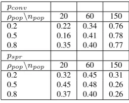
Table 3 summarizes the success rates on the Cassini test case for different values of

npopandρpopbut with all the heuristics active.

Table 3 Tuning ofnpopandρpopon the Cassini test case

pconv

ρpop\npop 20 60 150

0.2 0.22 0.34 0.76

0.5 0.16 0.41 0.78

0.8 0.35 0.40 0.77

pspr

ρpop\npop 20 60 150

0.2 0.32 0.45 0.31

0.5 0.45 0.48 0.26

0.8 0.37 0.40 0.26

One can see that the best convergence is obtained fornpop = 150and in particular when combined with ρpop = 0.5. On the other hand, best spreading is obtained with medium sized populations withnpop = 60. A good compromise seems to be

npop = 150andρpop = 0.2. Results on the other test cases (as shown in Table 4, Table 5 and Table 6, withnpop = 150andρpop = 0.2) show in general that large

populations and smallρpop are preferable. This also means that social actions on a

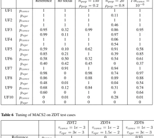
large quota of the populations are undesirable and it is better to perform social moves among a restricted circle of agents. Table 4 reports the results of the tuning of MACS2 on the 3-imp and Cassini test cases. Table 5 and Table 6 report the results of the tuning of MACS2 on the UF and ZDT test sets respectively.

Table 4 shows a marked improvement ofpconvon the Cassini when the population size is 150. Likewise, Table 5 shows that in general, with a population of 150 agents, there is an improvement in performance, and onpspr in particular, on the UF1, 2,

6, 8 and 9 test cases. Notable exceptions are the ZDT in Table 6, for which the best performance is obtained for a small population withnpop= 20.

The impact ofF is uncertain in many cases, however, Table 7 shows for example that on the UF8 test case a better performance is obtained for a high value ofF. Table 5 and Table 6 show that the default value forT olconvalready gives good performance and it does not seem advantageous to reduce it or make it larger.

The impact of social actions can be seen in Table 4, Table 5 and Table 6. Table 4 shows that on the 3-impulse and Cassini test cases the impact is clearly evident, since

Table 4 Tuning of MACS2 on the 3-impulse and Cassini test cases

3-impulse Cassini

pconv pspr pconv pspr

Reference 0.99 0.99 0.38 0.36

no social 0.47 1 0 0.18

npop= 150, ρpop= 0.2 1 1 0.76 0.31

F= 0.9 0.97 0.99 0.50 0.36

T olconv= 10−6 0.99 0.99 0.38 0.45

Table 5 Tuning of MACS2 on the UF test cases

Reference no social npop= 150 npop= 20 T olconv=

ρpop= 0.2 ρpop= 0.8 10−6

UF1 pconv 1 1 1 1 1

pspr 1 1 1 0.11 1

UF2 pconv 1 1 1 1 1

pspr 1 1 1 0.46 1

UF3 pconv 0.95 0.32 0.99 0.86 0.95

pspr 0.99 0.11 1 0.97 1

UF4 pconv 1 1 1 0.06 1

pspr 1 1 1 0.54 1

UF5 pconv 0.59 0.10 0.62 0.91 0.58

pspr 0.85 0.21 1 0.39 0.85

UF6 pconv 0.58 0.50 0.32 0.54 0.61

pspr 0.40 0.42 0.45 0 0.37

UF7 pconv 1 0.91 1 0.94 1

pspr 0.98 0 0.98 0.74 0.97

UF8 pconv 0.86 0 0.88 0.89 0.88

pspr 0.48 0.01 1 0.04 0.54

UF9 pconv 0.68 0.12 0.84 0.31 0.74

pspr 0.60 0 1 0 0.64

UF10 pconv 0 0.01 0 0.28 0.01

pspr 0 0 0 0 0

Table 6 Tuning of MACS2 on ZDT test cases

ZDT2 ZDT4 ZDT6

τconv= 1e−3 τconv= 1e−2 τconv= 1e−3

τspr= 3e−3 τspr= 1.5e−2 τspr= 3e−3

Reference pconv 1 0 0.93

pspr 1 0 1

no social pconv 1 0 0.91

pspr 1 0 0.98

npop= 150 pconv 0.20 0 0.60

ρpop= 0.2 pspr 0.17 0 1

npop= 20 pconv 1 0.02 0.96

ρpop= 0.8 pspr 1 0.02 1

F= 0.9 pconv 1 0 0.96

pspr 1 0 1

T olconv= 1e−6 pconv 1 0 0.96

pspr 1 0 1

MACS2 (Tuned) pconv 1 0 0.96

pspr 1 0 1

MACS pconv 0.82 0.81 0.63

pspr 0 0.93 0.0

Table 7 Tuning ofFon the UF8 test cases

UF8

F 0.1 0.5 0.9

there is a marked worsening of bothpconvandpspr. On the the UF benchmark, see Table 5, removing social actions induces a sizeable worsening of the performance metrics. This is true in particular for functions UF1, UF3, UF5, UF6, UF7, UF8 and UF9. Notable exceptions are UF2, UF4 and UF10. As a results of the tuning test cam-paign, the settings reported in Table 8 are recommended. Note that the recommended population size for all the cases except the ZDT functions, is 150 agents, while for the ZDT functions remains 20 agents.

Table 8 Settings for MACS2 after tuning.

npop ρpop F T olconv

150(20) 0.2(0.8) 0.9 10−4

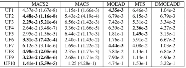
With these settings, the performance of MACS2 was compared, on the UF test suite in Table 9, with that of MACS, Multi objective Evolutionary Algorithm based on Decomposition (MOEAD, Zhang and Li (2007)), Multiple Trajectory Search (MTS, Tseng and Chen (2009)) and Dynamical Multi Objective Evolutionary Algorithm (DMOEADD, Liu et al (2009)). The last three are the best performing algorithms in the CEC09 competition (Zhang and Suganthan, 2009).

Table 9 Performance comparison on UF test cases: Average IGD (variance within parenthesis)

MACS2 MACS MOEAD MTS DMOEADD

UF1 4.37e-3 (1.67e-8) 1.15e-1 (1.66e-3) 4.35e-3 6.46e-3 1.04e-2

UF2 4.48e-3 (1.16e-8) 5.43e-2 (4.19e-4) 6.79e-3 6.15e-3 6.79e-3

UF3 2.29e-2 (5.21e-6) 6.56e-2 (1.42e-3) 7.42e-3 5.31e-2 3.34e-2

UF4 2.64e-2 (3.48e-7) 3.36e-2 (1.66e-5) 6.39e-2 2.36e-2 4.27e-2 UF5 2.95e-2 (1.56e-5) 6.44e-2 (1.17e-3) 1.81e-1 1.49e-2 3.15e-1

UF6 3.31e-2 (7.42e-4) 2.40e-1 (1.43e-2) 1.76e-1 5.91e-2 6.67e-2

UF7 6.12e-3 (3.14e-6) 1.69e-1 (1.22e-2) 4.44e-3 4.08e-2 1.03e-2

UF8 4.98e-2 (2.05e-6) 2.35e-1 (1.77e-3) 5.84e-2 1.13e-1 6.84e-2

UF9 3.23e-2 (2.68e-6) 2.68e-1 (1.71e-2) 7.90e-2 1.14e-1 4.90e-2

UF10 1.41e-1 (5.59e-5) 1.25 (4.28e-1) 4.74e-1 1.53e-1 3.22e-1

As shown in Table 9, the tuned version of MACS2 outperforms the other algorithms on UF2, 3, 6, 8, 9 and 10, on UF1 is very close to MOEAD, while it ranks second on UF5 and 10 and finally third on UF7.

In Table 6 one can find the comparison against the old version MACS on the ZDT test set. MACS2 results generally better except on the ZDT4 case. Note thatMspr

of MACS for both ZDT2 and ZDT6 is always between 0.6e-2 and 0.9e-2, therefore always above the chosen thresholdτspr.

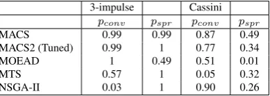
Table 10 Comparison of MACS, MACS2 and MOEAD on 3-impulse and Cassini test cases

3-impulse Cassini

pconv pspr pconv pspr

MACS 0.99 0.99 0.87 0.49

MACS2 (Tuned) 0.99 1 0.77 0.34

MOEAD 1 0.49 0.51 0.01

MTS 0.57 1 0.05 0.32

NSGA-II 0.03 1 0.90 0.26

With this modifications, a success rate of 0.66 both on convergence and spreading is achieved although thepconv andpspr on ZDT2 drops to 0 and thepconv on ZDT6 drops to 23%.

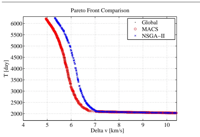
Table 10 shows a comparison of the performance of MACS2 on 3-impulse and Cassini, against MACS, MOEAD, MTS and NSGA-II. Both MACS and MACS2 are able to reliably solve the 3-impulse case, while MOEAD manages to attain good conver-gence but with only mediocre spreading. On the contrary, both MTS and NSGA-II achieve good spreading but worse convergence, indicating that their fronts are quite well distributed but probably too distant from the true Pareto front. Cassini is a rather difficult problem and this is reflected by the generally lower metrics achieved by most algorithms. Only MACS, MACS2 and NSGA-II reach a high convergence ratio, but for the last two, their spreading is still rather low. After inspection of each of the 200 Pareto fronts one can see that such a low spreading implies that the algorithm did not converge to the global Pareto front. Fig.1 illustrates the difference between MACS and NSGA-II. The behavior of MACS2 is similar to the one of NSGA-II. MACS achieves the best known value for objective function∆v. Both NSGA-II and MACS2 instead fall in the basin of attraction of the second best value for objective function∆v(Vasile et al, 2009).

The performance of MOEAD and MTS on Cassini is rather poor, with the former attaining only 50% convergence but with almost zeropspr; conversely, only one third of the latter’s runs are below the spreading threshold and almost none meets the con-vergence criterion.

5 Conclusions

4 5 6 7 8 9 10 2000

2500 3000 3500 4000 4500 5000 5500 6000

Pareto Front Comparison

Delta v [km/s]

T [day]

Global MACS NSGA−II

Fig. 1 Comparison of Pareto fronts for the Cassini case

seems reasonable to assume that a more flexible set of individualistic moves might improve MACS2. This is the subject of current developments. Also, from the tests performed so far the actual contribution of the utility function is uncertain and more investigations are underway.

The use of a selection operator based on Tchebycheff decomposition, instead, appears to be beneficial in a number of cases. In MACS2, in particular, agents operating at the extreme of the range of each of each objective are always preserved and forced to improve a subproblem. A better solution of the subproblems is expected to further improve convergence. One possibility currently under investigation is to make some agents use a directed search exploiting the directions defined by theλvectors.

References

Erfani T, Utyuzhnikov S (2011) Directed search domain: a method for even gener-ation of the Pareto frontier in multiobjective optimizgener-ation. Engineering Optimiza-tion 43(5):467–484

Fliege J, Drummond M, Svaiter B (2009) Newtons method for multicriteria optimiza-tion. SIAM Journal on Optimization 20(2):602–626

Gra˜na Drummond L, Svaiter B (2005) A steepest descent method for vector opti-mization. Journal of computational and applied mathematics 175(2):395–414 Ishibuchi H, Yoshida T (2002) Hybrid Evolutionary Multi-Objective Optimization

Knowles J, Corne D (1999) Local search, multiobjective optimization and the pareto archived evolution strategy. In: Proceedings of Third Australia-Japan Joint Workshop on Intelligent and Evolutionary Systems, Citeseer, pp 209–216, URL

http://citeseerx.ist.psu.edu/viewdoc/download?doi=10.1.1.33.6848&amp;rep=rep1&amp;type=pdf Kumar A, Sharma D, Deb K (2007) A hybrid multi-objective optimization procedure

using PCX based NSGA-II and sequential quadratic programming. In: Evolution-ary Computation, 2007. CEC 2007. IEEE Congress on, IEEE, pp 3011–3018 Lara A, Sanchez G, Coello Coello C, Schutze O (2010) HCS: A new local search

strategy for memetic multiobjective evolutionary algorithms. Evolutionary Com-putation, IEEE Transactions on 14(1):112–132

Laumanns M, Thiele L, Deb K, Zitzler E (2002) Combining convergence and diversity in evolutionary multiobjective optimization. Evolutionary computation 10(3):263–282

Liu M, Zou X, Chen Y, Wu Z (2009) Performance assessment of DMOEA-DD with CEC 2009 MOEA competition test instances. In: Evolutionary Computation, 2009. CEC’09. IEEE Congress on, IEEE, pp 2913–2918

Maddock C, Vasile M (2008) Design of optimal spacecraft-asteroid formations through a hybrid global optimization approach. International Journal of Intelligent Computing and Cybernetics 1(2):239–268

Minisci E, Avanzini G (2009) Orbit transfer manoeuvres as a test benchmark for com-parison metrics of evolutionary algorithms. In: Evolutionary Computation, 2009. CEC’09. IEEE Congress on, IEEE, pp 350–357

Rigoni E, Poles S (2005) NBI and MOGA-II, two

com-plementary algorithms for multi-objective optimizations. In:

Practical Approaches to Multi-Objective Optimization, URL

http://citeseerx.ist.psu.edu/viewdoc/download?doi=10.1.1.89.6798&amp;rep=rep1&amp;type=pdf Sanchez J, Colombo C, Vasile M, Radice G (2009) Multi-criteria comparison among

several mitigation strategies for dangerous near earth objects. Journal of Guidance, Control and Dynamics 32(1):121–142

Schuetze O, Sanchez G, Coello Coello C (2008) A new memetic strategy for the numerical treatment of multi-objective optimization problems. In: Proceedings of the 10th annual conference on Genetic and evolutionary computation, ACM, pp 705–712

Sch¨utze O, Laumanns M, Tantar E, Coello C, Talbi E (2010) Computing gap free pareto front approximations with stochastic search algorithms. Evolutionary Com-putation 18(1):65–96

Sindhya K, Sinha A, Deb K, Miettinen K (2009) Local search based evolutionary multi-objective optimization algorithm for constrained and unconstrained prob-lems. In: Evolutionary Computation, 2009. CEC’09. IEEE Congress on, IEEE, pp 2919–2926

Tseng L, Chen C (2009) Multiple trajectory search for unconstrained/constrained multi-objective optimization. In: Evolutionary Computation, 2009. CEC’09. IEEE Congress on, IEEE, pp 1951–1958

Vasile M, Locatelli M (2009) A hybrid multiagent approach for global trajectory optimization. Journal of Global Optimization 44(4):461–479

Vasile M, Zuiani F (2010) A hybrid multiobjective optimization algorithm applied to space trajectory optimization. In: Evolutionary Computation (CEC), 2010 IEEE Congress on, IEEE, pp 1–8

Vasile M, Zuiani F (2011) Multi-agent collaborative search: an agent-based memetic multi-objective optimization algorithm applied to space trajectory design. Proceed-ings of the Institution of Mechanical Engineers, Part G: Journal of Aerospace En-gineering 225(11):1211–1227

Vasile M, Minisci E, Locatelli M (2009) A dynamical system perspective on evolu-tionary heuristics applied to space trajectory optimization problems. In: Evolution-ary Computation, 2009. CEC’09. IEEE Congress on, IEEE, pp 2340–2347 Vasile M, Minisci E, Locatelli M (2010) Analysis of some global optimization

algo-rithms for space trajectory design. Journal of Spacecraft and Rockets 47(2):334– 344

Vasile M, Minisci E, Locatelli M (2011) An inflationary differential evolution algo-rithm for space trajectory optimization. Evolutionary Computation, IEEE Transac-tions on 15(2):267–281

Zhang Q, Li H (2007) MOEA/D: A multiobjective evolutionary algorithm based on decomposition. Evolutionary Computation, IEEE Transactions on 11(6):712–731 Zhang Q, Suganthan P (2009) Final report on CEC09 MOEA competition. In: IEEE

Congress on Evolutionary Computation, CEC’09

Zhang Q, Zhou A, Zhao S, Suganthan P, Liu W, Tiwari S (2008) Multiobjective op-timization test instances for the cec 2009 special session and competition. Univer-sity of Essex, Colchester, UK and Nanyang Technological UniverUniver-sity, Singapore, Special Session on Performance Assessment of Multi-Objective Optimization Al-gorithms, Technical Report

Zhang Q, Liu W, Li H (2009) The performance of a new version of MOEA/D on CEC09 unconstrained MOP test instances. In: Evolutionary Computation, 2009. CEC’09. IEEE Congress on, IEEE, pp 203–208