Multiple target three dimensional coordinate estimation for bistatic MIMO radar with uniform linear receive array

R E S E A R C H

Open Access

Multiple target three-dimensional coordinate

estimation for bistatic MIMO radar with uniform

linear receive array

Jun Li

, Huan Li

, Libing Long

, Guisheng Liao

and Hugh Griffiths

Abstract

A novel scheme to achieve three-dimensional (3D) target location in bistatic radar systems is evaluated. The proposed scheme develops the additional information of the bistatic radar, that is the transmit angles, to estimate the 3D coordinates of the targets by using multiple-input multiple-output techniques with a uniform circular array on transmit and a uniform linear array on receive. The transmit azimuth, transmit elevation angles and receive cone angle of the targets are first extracted from the receive data and the 3D coordinates are then calculated on the basis of these angles. The geometric dilution of precision which is based on the root Cramer-Rao bound of the angles, is derived to evaluate the performance bound of the proposed scheme. Further, an ESPRIT based algorithm is developed to estimate the 3D coordinates of the targets. The advantages of this scheme are that the hardware of the receive array is reduced and the 3D coordinates of the targets can be estimated in the absence of the range information in bistatic radar. Simulations and analysis show that the proposed scheme has potential to achieve good performance with low-frequency radar.

Keywords:Bistatic, MIMO radar, 3D coordinates, Circular array, GDOP

1. Introduction

Multiple-input multiple-output (MIMO) radar is a rela-tively new term in the radar field, inspired by the MIMO technique in communications. MIMO radar has multiple transmit channels and multiple receive channels, and the transmit channels can be separated by waveforms, or time, or frequencies, or polarizations at each receiver. So the number of channels of a MIMO radar is increa-sed substantially compared to its single-input multiple-output counterparts. Most of the advantages of the MIMO radar come from increasing the number of channels. Two main classes of MIMO radar have been proposed: with widely separated antennas [1] and with co-located antennas [2]. The first class utilizes the differ-ent scattering properties of a target from sufficidiffer-ently spaced antennas to improve the performance of the sys-tems. The second class allows the improvement of the

radar performances by coherent processing the multiple channels.

A scheme of bistatic MIMO radar has recently been proposed for target localization [3]. Bistatic MIMO radar has the potential advantages both of bistatic radar, such as reduced space loss, covert operation, and reduced susceptibility to jamming [4], and of MIMO radar, such as high spatial resolution and additional spatial degrees of freedom [2]. Also, bistatic MIMO radar has the par-ticular advantage of being able to obtain the target angles with respect to the transmit array (direction of departure) by processing the received data [3]. Several publications have studied direction of departure and di-rection of arrival estimation for bistatic MIMO radar [5-9]. Multiple target localization without range infor-mation can be achieved by using the estimated angles. However, only two-dimensional (2D) Cartesian coor-dinates can be obtained from the estimated 2D angles. In [10], both the transmit and the receive array are configured as uniform circular arrays UCAs. A trilinear decomposition-based algorithm is developed to estimate the four-dimensional angles of the targets in bistatic * Correspondence:junli01@mail.xidian.edu.cn

1

National Lab of Radar Signal Processing, Xidian University, Xi’an 710071, China

Full list of author information is available at the end of the article

MIMO radar. In fact, 3D angles are sufficient to locate the targets. It is well known that the localization per-formance of the bistatic radar is related to the location of the targets. However, to the best of the authors’ knowledge, there is no published work on evaluating the localization performance of bistatic MIMO radar in a Cartesian coordinate system.

In this article, a bistatic MIMO radar system with transmit UCA and receive uniform linear array (ULA) is constructed. The 3D coordinates of the targets are then obtained by estimating the transmit azimuth angle, transmit elevation angle and receive cone angle from re-ceive data. The geometric dilution of precision (GDOP) of the system is developed based on the Cramer-Rao bound (CRB) of the angles estimation. The ESPRIT algo-rithm with phase mode excitation is derived to estimate the 3D angles. The range of the target is not required in target 3D coordinates estimation and the time synchro-nization constraint of the bistatic radar is relaxed.

The reminder of the article is organized as follows. The bistatic MIMO radar system model is introduced in Section 2. In Section 3, the GDOP bound is developed to evaluate the performance potential of the proposed scheme. An ESPRIT-like algorithm is developed to esti-mate the 3D coordinates of the targets in Section 4. The proposed scheme is tested via simulations and analysis, which appear in Section 5. Finally, Section 6 concludes the article.

2. Bistatic MIMO radar system model

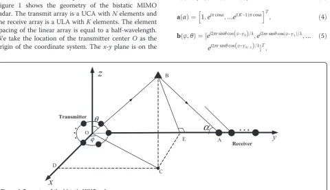
Figure 1 shows the geometry of the bistatic MIMO radar. The transmit array is a UCA withNelements and the receive array is a ULA withKelements. The element spacing of the linear array is equal to a half-wavelength. We take the location of the transmitter centerO as the origin of the coordinate system. The x-yplane is on the

ground plane and the z-axis points vertically upwards. For simplicity and without loss of generality, we put the receive ULA along they-axis.Ais the reference point of the receiver and the length of the baselineOAisLb. The elements of the transmitter are uniformly distributed over the circumference of a circle of radius rin thex-y

plane. The spacings of both transmit and receive array elements are a half-wavelength.α∈[0,π],θ∈0;π₂ and φ

∈ −π

2;π2

are the receive cone angle transmit elevation angle and transmit azimuth angle respectively.

Here, we assume that the transmitted waveforms

snð Þt

f gN

n ¼ 1 are orthogonal to each other, that is

∫smð Þt s_kðt−τÞdτ¼δmk ð1Þ

where (g)* denotes the conjugate operator.

Assume thatPtargets with the same range are distrib-uted over different angles. The received signal at thelth pulse period can be expressed as follows:

xlð Þ ¼t

XP

i¼1

ρiað Þαi bTðθi;φiÞsð Þt ej2πfDil

þwl; ð2Þ

where ρi is the signal-reflected coefficient of the i th target. (αi, θi, φi) denotes the corresponding angle of the

i th target and fDidenotes the Doppler frequency of the

i-th target.wlis Gaussian white noise with covarianceσ2.

sð Þ ¼t ½s1ð Þ;t s2ð Þt …sNð Þt T; ð3Þ

að Þ ¼α 1;ejπcosα;…ej Kð −1Þπcosα

h iT

; ð4Þ

bðφ;θÞ ¼ ½ej2πrsinθcosðφ−γ0Þ=λ;_ej2πrsinθcosðφ−γ1Þ=λ;…

ej2πrsinθcosðφ−γN−1Þ=λT;

ð5Þ

whereγn= 2πn/N,n= 0,…,N−1. The channel separation of the MIMO radar can be achieved by a bank of matched filters in the receiver [3]. The result at thelth pulse period is as follows:

Xð Þ ¼l X P

i¼1

ρiað Þαi bTðθi;φiÞej2πfDilþWl ð6Þ

Stacking the matrixX(l) as a vector, Equation (6) can be written in the form of theKN× 1 vector:

xl¼Ahþnl ð7Þ

where A= [a(α1)⊗b(φ1,θ1),a(α2)⊗b(φ2,θ2),…,a(αP)⊗ b(φP,θP)] and ⨂ denotes the Kronecker product. hl¼

ρ1ej2πfD1l;ρ2ej2πfD2l; ::::ρPej2πfDPl

T

.

ForLpulses, the signal model can be expressed as

Y¼AHþW ð8Þ

whereY = [x1,…,xL] with the size of KN × L.H= [h1,

h2,…,hL] and W= [n1,…,nL]. It has been proven that the matrix W has the same statistical properties as the receive noisewlin the case of orthogonal transmit wave-forms [11].

3. Performance bound of the estimation

3.1. CRB of the 3D angles

The CRB provides a lower bound of the mean square error of the angle estimation by any unbiased estimator. Following the approach in [12], the CRB for 3D angles of multiple targets is calculated here to obtain the bound of angle estimation of the proposed scheme. The Fisher information matrix (FIM) for the angles can be calcu-lated as follows:

Fð Þ ¼ξ FF12;;11 FF21;;22 FF21;;33 F3;1 F3;2 F3;3 2

4

3

5 _ð9Þ

where ξ = [α,φ,θ]. α¼½α1 α2 ⋯ αΡ , φ¼

φ1 φ2 ⋯ φΡ

½ and θ¼½θ1 θ2 ⋯ θΡ. The de-rivation of the submatrices of the FIM can be found in Appendix 1. The CRB of the 3D angles of the targets can be obtained by inverting the FIM

Cð Þ ¼ξ diagF−1ð Þξ ð10Þ

where diag(g) denotes a vector constructed by the diag-onal elements of matrix.

3.2. GDOP

As the localization performance of bistatic radar de-pends on the location of the target, we will analyze the estimate error of the 3D coordinates of the targets in dif-ferent location. The uncertainties of the measured angles

will propagate to the coordinate values according to the error propagation equation [13] as follows:

Δe¼T−1_{Δv ð11Þ}

whereΔe = [Δx,Δy,Δz]Tis the error of the coordinates.

Δv = [Δα,Δθ,Δφ]Tis the error of the estimated angles. T is the error propagation matrix which is derived in Appendix 2. The performance bound of the 3D coordi-nates estimation can be obtained from (11) by using the root Cramer-Rao bound (RCRB) as the error of the esti-mated angles, that is

Δe¼T−1pffiffiffiffi_{C ð12Þ}

whereΔe¼½Δx;Δy;ΔzT. The GDOP metric for 3D co-ordinates is defined as follows:

GDOP¼

ffiffiffiffiffiffiffiffiffiffiffiffiffiffiffiffiffiffiffiffiffiffiffiffiffiffiffiffiffiffiffiffiffiffi

Δx2_þΔy2_þΔz2 q

ð13Þ

In fact, Equation (13) described the bound of the root mean square error (RMSE) of the 3D coordinate estima-tion of the target at difference locaestima-tion.

3.3. Analysis of the performance bound

The GDOPs of the proposed scheme are plotted in Figure 2. The GDOPs in the plane of z= 35 km are plot-ted according to (12) and (13). T and R in the Figure indicate the locations of transmitter and receiver re-spectively. T is located at the origin of the coordinates system and R is located at [0, 100 km, 0]. The Figure shows the performance bound of the proposed scheme. It can be observed that the performance of 3D coordi-nates estimation varies with the range between the target and the transmitter. It can be seen in Figure 2 that the estimation error can reach several meters when the range of the target is within 50 km and tens of meters when the range of the target is within 150 km. When the signal-to-noise ratio increases the performance is even better. This performance is to be expected in the case of the radar with large signal bandwidth. However, this performance is good in the case of low-frequency radar, for example when the wavelength of the transmit signal is 15 m or more, as there is not enough signal band-width to provide accurate range estimation. Fortunately, the performance of the 3D coordinate estimation can be achieved without the range information by the proposed scheme. So, the proposed scheme is suitable for low-frequency radar.

element spacing, more elements mean greater aperture. If the spacing is a half-wavelength and the wavelength is 15 m, the aperture would be 150 m for 20 elements, which implies several technological issues to translate into a real system design. Recently proposed bio-inspired couple compact array can reduce the elements spacing considerably and keep high direction of arrival estimation

performance [14]. It is a promising technique to resolve this problem.

4. Target 3D coordinates estimation method

In this section, we develop an ESPRIT-like algorithm to estimate the 3D angles of the targets.

4.1. Estimation of the receive cone angles

To estimate the receive cone angle, we first construct se-lection matricesJ1andJ2.

J1¼IN⊗ IK−1;0ðK−1Þ1

ð14Þ

J2¼IN⊗ 0ðK−1Þ1;IK−1

ð15Þ

where IK−1 and IN are identify matrices with size K–1 and N, respectively. 0ðK−1Þ1 denotes a zero vector with sizeK–1.

The rotated factor which contain the receive cone angle can be obtained by using selection matrices as fol-lows:

Y1¼J1Y¼J1AHþJ1W ð16Þ Y2¼J2Y¼J2AHþJ2W¼J1ADHþJ2W ð17Þ

where the rotated factor is D¼diag e½ jπcosα1; _ejπcosα2…

ejπcosαP_.

The autocorrelation and crosscorrelation matrices of Y1andY2are as follows:

R11¼E Y1Y1H

¼J1ARsAHJ1HþRW1 ð18Þ R21¼E Y2Y1H

¼J1ADRsAHJ1H ð19Þ

where Rs=E[HHH] and RW1=σ2INK−1. As proved in [11], the noise covariance σ here is the same as that at the MIMO radar receiver. It can be obtained when there

is no input signal in the receiver. So the effect of noise can be cancelled as follows:

R11s¼R11−σ2INK−1¼J1ARsAHJ1H ð20Þ DefineAr=J1Aand construct the matrixR¼R21R#11s,

where R#_11s is the Penrose-Moore inverse of R11s. Just as in the method proposed in [15], we can write

RAr¼ArD ð21Þ

Estimates of the receive cone angles are achieved via eigendecomposition of R as

R¼UΛUH _ð22Þ

where Λ= diag[λ1,λ2,⋯,λP] is constructed by the ma-ximum P eigenvalue of R. The number of targets P

should be estimated in advance. The issue of the target number detection for bistatic MIMO radar can be found in [16]. From (21) and (22), the receive angle of thepth target is

αp¼ arccos

angleð Þλi π

ð23Þ

4.2. Estimation of the transmit angles

From (21) and (22), we can obtain that span{Ar} = span {U}. So the transmit angle information can be extracted fromU= [u1,⋯,uP]. The vector ~a should be first cons-tructed to separate the transmit angle information of the

pth target from the matrixupas follows:

~

a αp ¼kron 1;…;1

N

T

;ar αp ð24Þ

~

yp¼up⊙~a αp ð25Þ

where⊙denotes hadamard product andar(αp) is a vec-tor constructed by the first K–1 elements of a(αp). Di-vide ~y_p into K–1 vectors with the size of N× 1 and average the vectors as follow:

y_p ¼ 1 K−1

XK−1

k¼1 ~

y_k;~y_ðK−1Þþk⋯;~y_{ðN−1ÞðK−1Þþk}

h iT

ð26Þ

Then UCA-ESPRIT algorithm can be used to esti-mate the transmit azimuth angle and elevation angle. The phase mode excitation method is exploited to sim-plify the array manifold of the circular array. The beam-former matrix FH_r is constructed to transform the UCA manifold vector to the beamspace manifold [17].

FH

r ¼G

H_C

vVH ð27Þ

where Cv=diag(j−M,…j−1,j0,j−1,....j−M). M≈2πr_λ is the highest order mode that can be excited by the aperture

5 10 15 20

12 14 16 18 20 22 24

the number of the receive elements

R

M

SE(

m

)

Figure 3Influence of the number of the receive elements (N= 20,Lb= 100 km,r=λ, target: [100 km, 50 km,

at a reasonable strength. G¼pffiffiffiffiffiffiffiffiffiffi_2M1_{þ1½wða−MÞ;…; wð Þ;a0} …;wðaMÞ, where am¼ 2πm

2Mþ1;m∈ −M½ ;M and ð Þ ¼am

e−jMam;…;_e−jam;_ej0am;_ejam;…;_ejMam

½ T

.V¼ 1ffiffiffi

N

p ½_v−M;…_v0; …vM, wherevm = [1,ej2πm/N,…,ej2πm(N−1)/N]H.

The selected data after transformation is as follows:

yp¼FHryp ð28Þ

The sample covariance matrix can be calculated as fol-lows:

Rp ¼

1

Lypy H

p; p¼1;2;…;P ð29Þ

EVD of the matrix Re(Rp) is performed to obtain the real-value signal subspacespwhich is the eigenvectors of the largest eigenvalue of the matrix Re(Rp). Re(●) de-notes the real part of the elements of the matrix.Ptimes EVD should be performed separately to estimate P

eigenvector.

Transform the real-value signal subspace as follows:

s0¼C0Wsp ð30Þ

where C0¼diag ð Þ−1 N;…;ð Þ−1 1;1;1;…;1 zfflfflfflfflffl}|fflfflfflfflffl{Mþ1 8

< :

9 =

; . Define

sð Þ−1 0 ands

0 ð Þ

0 as the first and the last 2M–1 elements of the vectors0respectively. The following equation can be founded [17]

Eu^¼Γsð Þ₀0 ð31Þ

where E¼ s0ð Þ−1 D^Isð Þ0−1

h i

and Γ¼_πrλdiagf−ðM−1Þ; …;0;…;ðM−1Þg.D = diag{(−1)M−2,…, (−1)1, (−1)0, (−1)1, …, (−1)M} and ^I is the reverse permutation matrix with ones on the anti-diagonal and zeros elsewhere. The least

square solution of (30) is^uLS¼ ^up u^p

h iT

.

The transmit azimuth angles and elevation angles can be obtained fromup^ ;p¼1;2;…P, asup^ ¼ sinθpejφp_[17].

So, the azimuth anglesφpand elevation angles θpcan be calculated from the following formulas.

φp¼ arg ^up ð32Þ

θp ¼arcsin^up ð33Þ

The receive angles and transmit angles can be paired automatically as they are connected by the correspon-ding eigenvalues and eigenvectors, respectively.

4.3. 3D coordinates of the targets

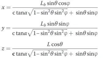
In this section, the 3D coordinates are calculated by the angles estimated in Sections 4.1 and 4.2. The relation-ship between [α, φ, θ] and 3D coordinates of the target [x,y,z] can be found by the geometry of bistatic MIMO radar in Figure 1 as follows:

x¼ Lbsinθcosφ

c tanαpffiffiffiffiffiffiffiffiffiffiffiffiffiffiffiffiffiffiffiffiffiffiffiffiffiffiffiffi1−sin2θsin2φþ sinθsinφ ð34Þ

y¼ Lbsinθsinφ

c tanαpffiffiffiffiffiffiffiffiffiffiffiffiffiffiffiffiffiffiffiffiffiffiffiffiffiffiffiffi1−sin2θsin2φþ sinθsinφ ð35Þ

z¼ Lcosθ

ctanαpffiffiffiffiffiffiffiffiffiffiffiffiffiffiffiffiffiffiffiffiffiffiffiffiffiffiffiffi1−sin2_θsin2_{φþ sinθsinφ} ð36Þ It can be observed that the 3D coordinates of the tar-gets are determined by the 3D angles estimated above and the baseline of the bistatic radar.

5. Simulation and analysis

In this section, we demonstrate via simulations the performances of the proposed scheme. As shown in Figure 1, a transmit UCA with radius r=λ is employed for the simulations and the number of the transmit ele-ments is selected as N= 20. The receive array is a ULA with 20 elements spaced at a half-wavelength. The base-line between transmitter and receiver is 100 km. In these simulations, we assume a low-frequency radar system. The transmit signals are narrowband and centered at 20 MHz (λ= 15m). We first estimate the transmit azi-muth angle, transmit elevation angle, and receive cone angle by the proposed method and then calculate the 3D coordinates of the targets according to the angles. The localization performance is evaluated by the RMSE of the estimated values. Five hundreds Monte Carlo trials are performed.

5.1. Simulation 1: the influence of the SNR

achieve meter-level locate accuracy which is far less than the wavelength of the transmit signal. It can be observed that the estimation performances of the two targets are different from each other as the localization perform-ance of the bistatic radar is related to location of the targets.

5.2. Simulation 2: the identifiability of the adjacent targets

The identifiability of two adjacent targets is investigated by the simulation. Targets 1 and 2 are at the same range cell in the plane z= 35 km. Target 1 is located at (73.5 km, 34.094 km, 35 km). Target 2 changes its loca-tion along the isorange ellipse of bistatic radar as shown in Figure 5. TheΔxin Figure 6 denotes the difference of the x-coordinate between targets 1 and 2. The norma-lized Doppler frequencies of the two targets are selected as 0.1 and 0.9, respectively. It is shown in Figure 6(a)(b) that the estimation performance of target 1 is improved when target 2 is far away from it by using the proposed algorithm. However, the influence of the target 2 can be ignored when Δx> 0.4 km. It can also be observed that the estimation performance of target 1 declines consid-erably whenΔxis within 0.05 km. The results imply the identifiability of the two adjacent targets by using the proposed algorithm. While the RMSE of the proposed algorithm tends to increase in proximity of the x-axis origin, the RCRB maintains flat behavior. The reason is that the proposed algorithm can only distinguish the

70 70.5 71 71.5 72 72.5 73 73.5 74 10

20 30 40 50 60 70 80 90

x

y

isorange ellipse locus of target 2

location of the target 1

Figure 5The location relationship between target 1 and target 2.

5 10 15 20 25

10-6 10-5 10-4 10-3 10-2

SNR(dB)

R

M

S

E

(r

ad)

Proposed - receive cone Proposed - transmit elevation Proposed - transmit azimuth RCRB - receive cone RCRB - transmit elevation RCRB - transmit azimuth

(a)

5 10 15 20 25

10-6 10-5 10-4 10-3 10-2

SNR(dB)

RM

S

E

(

ra

d

)

Proposed - receive cone Proposed - transmit elevation Proposed - transmit azimuth RCRB - receive cone RCRB - transmit elevation RCRB - transmit azimuth

(b)

(c)

5 10 15 20 25

10-3 10-2 10-1 100

SNR(dB)

RM

S

E

(k

m

)

Proposed - target 1 Bound - target 1 Proposed - target 2 Bound - target 2

Figure 4Localization performance v.s SNR (K= 20,N= 20, Lb= 100 km,r=λ).(a) performance of the angle estimation of the

two targets by their angles. However, there still are other different characteristic of the two targets, such as reflec-tion coefficient and Doppler frequency. The behavior of the RCRB implies that the targets can be distinguished by these characteristic in theory. Furthermore, Equation (38) in Appendix 1 discloses the behaviour of the RCRB

in mathematical terms. It can be observed that the Fisher submatrix is a Hadamard product of A_H

αR−W1A_α and RT

s, whereA_HαR−W1A_α contains the angle information and RT_s contains the reflection coefficient and Doppler frequency of the targets. Full rank of RT_s can guarantee

0 0.1 0.2 0.3 0.4 0.5

10-6 10-5 10-4 10-3 10-2 10-1 100 101

Δx (km)

RM

S

E

(r

a

d

)

Proposed - receive cone Proposed - transmit elevation Proposed - transmit azimuth RCRB - receive cone RCRB - transmit elevation RCRB - transmit azimuth

(a)

0 0.1 0.2 0.3 0.4 0.5

10-3 10-2 10-1 100 101 102 103 104

Δx (km)

RM

S

E

(k

m

)

Proposed target 1 Bound target 1

(b)

Figure 6Identifiability of adjacent targets (K= 20,N= 20,Lb= 100 km,r=λ, SNR = 25 dB, target 1 at (73.5 km, 34.094 km, 35 km),

the full rank of the Fisher Matrix, even though the matrix A_H

αR−W1A_α tends to rank defect in the case of two adjacent targets.

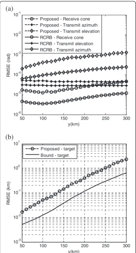
5.3. Simulation 3: influence of target range

The relationship between the estimation performances and target range is investigated in this subsection. As-sume the x and z coordinates of the target are fixed at

x= 50 km andz= 35 km respectively. The target location is changed along the y-axis from 50 km to 300 km. The signal-to-noise ratio is 25 dB. Figure 7(a) and (b) plots the performances of the angle and corresponding 3D co-ordinate estimation respectively. The dashed lines are the results of the proposed algorithms and the solid lines are the RCRB. It is shown that from both the proposed algorithm and the RCRB that the angle estimation per-formances vary little with the target range. However, the performance of the 3D coordinate estimation degrades with increasing target range. This simulation result is consistent with the analysis of the GDOP in Section 3.3. It seems that the proposed scheme is suitable to locate the target at relatively short range.

6. Conclusions

The transmit UCA and receive ULA configuration scheme for bistatic MIMO radar have been proposed to achieve target 3D localization. The performance bound of this scheme is evaluated and an ESPRIT-like al-gorithm was developed to achieve the 3D coordinate estimation of multiple targets. The advantage of the pro-posed scheme is that the 3D coordinates of multiple tar-gets can be estimated without the range information and has the capability for identification of multiple targets in the same range cell. Moreover, it is suitable for low-frequency radars to estimate the location of relatively short range targets. How to reduce the receive element spacing as well as keeping high angle estimation per-formance is the focus of our future work.

Appendix

A 1: Derivation of the FIM

In this section, the submatrices of FIM in (9) are derived. The (i,j)thelements of the submatrixF1,1are [12] notes the kronecker product. Re{g} denotes the real part of the data and tr{g} denotes the trace of the matrix. ei denotes a column vector with 1 at the ith element and zeros at the others. So we can obtain

F1;1¼2LRe A_H_αR−W1A_α

Proposed - Receive cone Proposed - Transmit azimuth Proposed - Transmit elevation RCRB - Receive cone RCRB - Transmit elevation RCRB - Transmit azimuth

(a)

In a similar way to the derivation above, we can obtain the other submatrices of the FIM as follows:

F1;2¼

Appendix 2. derivation of the error propagation matrix

The relationships between the 3D coordinates and the 3D angles are as follows:

α¼ arccos ffiffiffiffiffiffiffiffiffiffiffiffiffiffiffiffiffiffiffiffiffiffiffiffiffiffiffiffiffiffiffiffiffiffiffiLb−y

The elements of the error propagation matrix C are as follows:

The authors declare that they have no competing interests.

Acknowledgments

This study has been supported by the National Natural Science Foundation of China under contract No. 61271292 and the Fundamental Research Funds for the Central Universities. The authors are grateful to the anonymous referees for their constructive comments and suggestions in improving the quality of this paper.

Author details 1

National Lab of Radar Signal Processing, Xidian University, Xi’an 710071, China.2_{Department of Electronic and Electrical Engineering, University}

College London, London WC1E 6BT, UK.

References

1. A Haimovich, R Blum, L Cimini, MIMO radar with widely separated antennas. IEEE Signal Processing Magazine25, 116–129 (2008)

2. L Jian, P Stoica, MIMO radar with colocated antennas. IEEE Signal Processing Magazine24, 106–114 (2007)

3. Y Haidong, L Jun, L Guisheng,“Multitarget identification and localization using bistatic MIMO radar systems. EURASIP Journal on Advances in Signal Processing2008, 8 (2008). Article ID 283483

4. NJ Willis, HD Griffiths,Advances in Bistatic Radar(SciTech Publishing, Raleigh, NC, 2007)

5. M Jin, G Liao, J Li, Joint DOD and DOA estimation for bistatic MIMO radar. Signal Processing89(2), 244–251 (2009)

6. J Chen, G Hong, S Weimin, A new method for joint DOD and DOA estimation in bistatic MIMO radar. Signal Processing90(2), 714–718 (2010) 7. D Nion, ND Sidiropoulos, Adaptive algorithms to track the PARAFAC

decomposition of a third-order tensor. IEEE Trans. on Signal Processing

57(6), 2299–2310 (2009)

8. ML Bencheikh, W Yide, H Hongyang,“Polynomial root finding technique for joint DOA DOD estimation in bistatic MIMO radar. Signal Processing

90(no.9), 2723–2730 (2010)

9. XF Zhang, ZY Xu, LY Xu, DZ Xu,“Trilinear Decomposition-based Transmit Angle and Receive Angle Estimation for MIMO radar”, IET Radar. Sonar & Navig.5(6), 626–631 (2011)

10. X Zhang, X Gao, G Feng, D Xu, Blind joint DOA and DOD estimation and identifiability results for MIMO radar with different transmit/receive array manifolds. Progress in Electromagnetics Research B18, 101–109 (2009) 11. L Jian, X Luzhou, P Stoica, KW Forsythe, DW Bliss, Range compression and

waveform optimization for MIMO radar: a Cramer-Rao bound based study. IEEE Trans. on Signal Processing50(no.1), 218–232 (2008)

12. P Stoica, RL Moses,Spectral Analysis of Signals(Prentice-Hall, N.J., 1997) 13. R Philip, D Bevington, K Robinson,Data Reduction and Error Analysis for the

Physical Sciences(McGraw-Hill, New York, 2003)

14. M Akcakaya, CH Muravchik, A Nehorai, Biologically inspired coupled antenna array for direction of arrival estimation. IEEE Trans. on Signal Processing59(10), 4795–4808 (2011)

15. QY Yin, RW Newcomb, LH Zou, Estimating 2-D angle of arrival via two parallel linear array, inProc. of IEEE International Conference on ASSP

(IEEE, College Park, 1989), pp. 2803–2806

16. L Jun, L Guisheng, J Ming, M Qian,Multitarget detection and localization method for bistatic MIMO radar(Proceedings of IET International Radar Conference 2009, Guilin, China, 2009)

17. CP Mathews, MD Zoltowski, Eigenstructure techniques for 2-D angle estimation with uniform circular array. IEEE Trans. on Signal Processing

42(9), 2395–2407 (1994)

doi:10.1186/1687-6180-2013-81

Cite this article as:Liet al.:Multiple target three-dimensional coordinate estimation for bistatic MIMO radar with uniform linear receive array.EURASIP Journal on Advances in Signal Processing2013 2013:81.

Submit your manuscript to a

journal and benefi t from:

7 Convenient online submission 7 Rigorous peer review

7 Immediate publication on acceptance 7 Open access: articles freely available online 7 High visibility within the fi eld

7 Retaining the copyright to your article