http://www.gjaets.com
(C) Global Journal of Advance Engineering Technology and Science
Global Journal of Advance Engineering Technologies and Sciences
POWER SYSTEM FREQUENCY ESTIMATION USING DIFFERENT
ADAPTIVE FILTERSALGORITHMS FOR ONLINE VOICE
Rohini Pillay
1, Prof. Sunil Kumar Bhatt
2M. Tech. Scholar
1, Asst. Prof. & HOD
2Department of Electrical & Electronics Engineering
Central India Institute of Technology, Indore (M.P.) India
ABSTRACT
The Electrical power system frequency is an important parameter. The frequency of operation is not constant but it varies depending upon the load conditions. In the operating, controlling and monitoring of electric devices power system parameters are having great contribution. So it is very important to accurately measure this slowly varying frequency. Under steady-state conditions the total power generated by power stations is equal to system load and losses. Frequency can deviate from its nominal value due to sudden appearance of generation-load mismatches. Frequency is a vital parameter which influences different relay functionality of power system.
In this paper study was made to estimate the frequency of measuring voltage or current signal in presence of random noise and distortion. Here we are first using linear techniques such as least mean square (LMS), algorithm for measuring the frequency from the distorted voltage signal. Then comparing these results with nonlinear techniques such as nonlinear least mean square (NLMS), and UNANR algorithms with different modulation techniques was Amplitude Modulation. Signal performance parameter PSNR measured and compared with respect to Signal to Noise Ratio. The performances of these algorithms are studied through MATLAB R2013a simulation.
INTRODUCTION
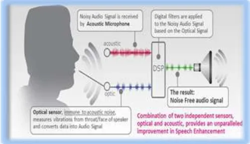
The speech enhancement technology has grown widely in telecommunication. There are lots of speech enhancement software in the market which improves the performance of the speech recognition but speech recognizers have various problems like noise interference, noise distortion which degrades the speech signal in communication system. In real time environment speech signal are corrupted by several forms of noise such as manmade noise examples car noise, background noise and also they are subjected to distortion caused by communication channels; examples are room reverberation, low-quality microphone, etc. In all such situations extraction of high resolution signals is a key task. It has many applications; for examples, mobile communications, robust speech recognition and low quality audio devices. Basically filtering techniques are broadly classified as adaptive and the non-adaptive filtering techniques. In practical cases the statistical nature of all speech signal is non-stationary; as a result non adaptive filtering may not be suitable. The first adaptive noise cancelling systems at Stanford University was designed and built in 1965 by two students. Their work was undertaken as part of the term paper project for a course in adaptive systems given by the Electrical Engineering Department. Since 1965, the adaptive noise cancelling has been successfully applied to a number of applications. [2-3].
Speech is a natural and the basic way for humans to convey message and thoughts. Speech frequency normally ranges between 3 Hz to 4 KHz depending upon the characters. However the human beings have audible frequency range of 20 Hz to 20 KHz. The most common problem in speech processing is effect of meddling of noise in the speech signals. The noise masks the speech signal reduce the quality and the speech is greatly affected by presence of backdrop noise. This make the listening task difficult for the straight listeners and gives poor performance in some of speech processing like speech recognition ,the speech coder and speaker identification etc. Noise shrinking or speech enrichment algorithm is to improve the performance of the communication systems when their input or output signals are corrupted by noise signal.
http://www.gjaets.com
(C) Global Journal of Advance Engineering Technology and Science
differently for each application. Two criteria are used to measure the performance: quality and intelligibility. It is very hard to satisfy both at the same time.
A. Speech Enhancement
The goal of speech enhancement is to empower speech quality by using several algorithms. It is one of the significant topics to enhance the performance of the systems of noisy in speech signal processing. It has many applications like cellular environments, telecommunication signal enhancement, military, front-ends for speech recognition system etc. The main objective of speech enhancement technique is to improve the quality and minimize the loss in intelligibility of the signals and listener fatigue. Various techniques are modeled for this purpose to improve speech signal to noise ratio and the performances depend on quality and intelligibility of the processed speech signal. The following figure 1 show the basic idea of speechenhancement.
There are many speech enhancement method proposed for noise reduction and to improve the noise quality and intelligibility. The earliest work in adaptive noise cancelling known to the author was performed by Howells and Applebaum and their colleagues at the General Electric Company between 1957 & 1960. They designed and built a system for antenna side lobe cancelling that used a reference input derived from an auxiliary antennas and a simple two-weight adaptive filter. In 1959, Widrow and Hoff were devised the LMS adaptive algorithm and the pattern recognition scheme known as ADALINE (for the “adaptive linear thresholds logic elements”). Hundreds of paper on adaptation, adaptive controls, adaptive filtering, and adaptive signal processing appeared in the literature. The best known commercial application of adaptive filtering grew from the work during these periods of Lucky at the Bell Laboratories. The adaptive noise cancelling system at Stanford University was design and built in 1965 by two students. Since 1965, adaptive noise cancelling has been successfully applied to a number of application. Several methods have been reported so far in the literature to enhance the performance of speech processing systems some of the most important ones are: Wiener’s filtering, LMS filtering, spectral subtraction, On the other side, LMS-based adaptive filter have been widely used in speech enhancement.Here few references papers are discussed as they have become a source of literature survey of this dissertation work.
Fig. 1: Basic Speech Enhancement System
In the another things Continuous improvement of communication and multimedia system has led to the widespread use of speech recording and processing device, e.g., mobile phones, speech recognition tools. In most practical situation, these devices are being used in environment where undesirable background noise exist. Degraded speech can cause problems for both mobile communication & speech recognition systems. Nowadays, all the people use the communication device almost as a primary goods: telephones, mobiles, internet and the customers demand a high coverage and quality.
B. Echo in Electrical System
http://www.gjaets.com
(C) Global Journal of Advance Engineering Technology and Science
1. Electrical echo: caused by the impedance mismatch at the hybrids transformer which the subscriber two-wire lines are connected to telephone exchange four wire lines in the telecommunication systems.
2. Acoustic Noise in Electrical System: Acoustic noise problems like industrial equipment noise, contending speakers, background noise, car engine noise, room reverberation, low-quality microphones are subjected on speech signals in real time surroundings. Speech signals are corrupted by these several forms of noise and also they are subjected to distortion caused by communication channels. Traditionally, acoustic noise cancellation used to apply passive techniques such as enclosures, barriers and silencers to remove the unwanted noise signal. Silencers were important for noise cancellation over broad frequency range but expensive and not efficient at low frequencies.
ADAPTIVE FILTERS
Digital signal processing (DSP) has been a major player in the current technical advancements such as noise filtering, system identification, voice prediction and echo cancellation. Standard DSP techniques, however, are not enough to solve these problems quickly and obtain acceptable results. Adaptive filtering techniques must be implemented to promote accurate solutions and a timely convergence to that solution. Adaptive Filter Adaptive filter is the most important component of acoustic noise canceller and it plays a key role in acoustic echo or noise cancellation. It performs the work of estimating the echo path of the room for getting a replica of echo signal. It requires an adaptive update to adapt to the environmental change. Another important thing is the convergence rate of the adaptive filter which measures that how fast the filter converges for best estimation of the room acoustic path. Adaptive filters are classified into two main groups: linear and nonlinear. Linear adaptive filters compute an estimate of a desired response by using a linear combination of the available set of observables applied to the input of the filter. Otherwise, the adaptive filter is said to be nonlinear.
A. Power system frequency estimation using LMS Algorithms
In 1959, Widow and Hoff derived an algorithm whose name was Least Mean Square (LMS) algorithm and till now it is one of the best adaptive filtering algorithms. This algorithm is used widely for different application such as channel equalization and echo cancellation. This algorithm adjusts the coefficients of (W)nof a filter in order to
reduce the mean square error between the desired signal and output of the filter. This algorithm is basically the type of adaptive filter known as stochastic gradient-based algorithms. Why it’s called stochastic gradient algorithm? Because in order to converge on the optimal Wiener solution, this algorithm use the gradient vector of the filter tap weights. This algorithm is also used due to its computational simplicity.
The LMS algorithm is a method to estimate gradient vector with instantaneous value. It changes the filter tap weights so that e(n) is minimized in the mean-square sense. The conventional LMS algorithm is a stochastic implementation of the steepest descent algorithm. It simply replaces the cost function ξ(n) = E[e2(n)] by its instantaneous coarse estimate.
Coefficient updating equation 1 for LMS is given by:
w(n + 1) = w(n) +μ i(n)e(n)1
Where µ is a step-size parameter and it controls the immediate change of the updating factor. It shows a great impact on the performance of the LMS algorithm in order to change its value. If the value of µ is so small then the adaptive filter takes long time to converge on the optimal solution and in case of large value the adaptive filter will be diverge and become unstable.
B. Mathematical Derivation of the LMS algorithm
The derivation of LMS algorithm is the development of the steepest decent method and also takes help from the theory of Wiener solution (optimal filter tap weights). This algorithm is basically using the formulas which updates the filter coefficients by using the tap weight vectors w and also update the gradient of the cost function accordingly to the filter tap weight coefficient vector∇ξ(n). From Equation (2) in the steepest decent algorithm,
w(n + 1) = w(n) −μ∇ξ(n) 2
w(n + 1) = w(n) +μE{e(n)x(n)} 3
In practice, the value of the expectation E{e(n)x(n)}is normally unknown, therefore we need to introduces the approximation or estimated as the sample mean
Ě{e(n)x(n)} =1
L∑ e(n − l)x(n − l) L−1
i=0 4
With this estimate we obtain the updating weight vector as,w(n − 1) = w(n) +µ
L∑ e(n − l)x(n − l) L−1
i=0 5
http://www.gjaets.com
(C) Global Journal of Advance Engineering Technology and Science
w(n + 1) = w(n) + μe(n)x(n) 7
C. Power system frequency estimation using Normalized LMS
Normalized Least Mean Square (NLMS) is actually derived from Least Mean Square (LMS) algorithm. The need to derive this NLMS algorithm is that the input signal power changes in time and due to this change the step-size between two adjacent coefficients of the filter will also change and also affect the convergence rate. Due to small signals this convergence rate will slow down and due to loud signals this convergence rate will increase and give an error. So to overcome this problem, try to adjust the step-size parameter with respect to the input signal power. Therefore the step-size parameter is said to be normalized.
It is another class of adaptive algorithm used to train the coefficients of the adaptive filter. This algorithm takes into account variation in the signal level at the filter output and selecting the normalized step size parameter that results in a stable as well as fast converging algorithm. The weight update relation for NLMS algorithm is as follows equation 8.
w(n + 1) = w(n) + μ(n) i(n) e(n) 8
By using this normalized step-size parameter in Least Mean Square algorithm, this algorithm is known as Normalized Least Mean Square (NLMS) algorithm. The step size for computing the update weight vector is, the variable step can be written as in equation 9.
μ(n) = β
C+‖X(n)‖2 9
Where:
μ(n) is step-size parameter at sample n
β is normalized step-size (0 < 𝛽 < 2)
𝐶is safety factor (small positive constant).
The advantage of the NLMS algorithm is that the step size can be chosen independent of the input signal power and the number of tap weights. Hence the NLMS algorithm has a convergence rate and a steady state error better than LMS algorithm.
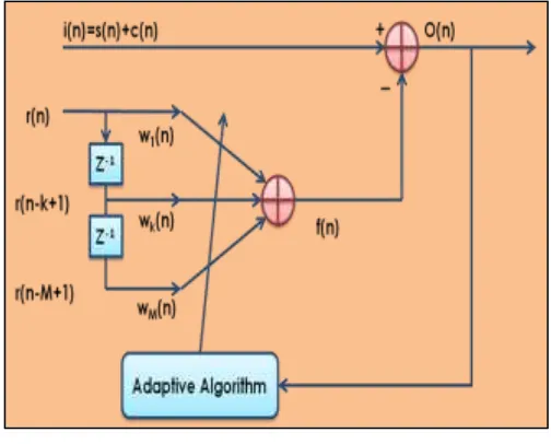
D. Adaptive Noise Reduction in UNANR algorithm
The UNANR model of the system performs the function of adaptive noise estimation. The UNANR model of order M, as shown in figure 2, is a transversal, linear, finite impulse response (FIR) filter. The response of the filter f(n) at each time instant (sample) n can be expressed as,
𝑓(𝑛) = ∑𝑀𝑚=1𝑊𝑚(𝑛)𝑟(𝑛 − 𝑚 + 1) 10
Where 𝑊𝑚 (n) represents the UNANR coefficients, and r(n − m + 1) denotes the reference input noise at the present
(m = 1) and preceding m − 1, (1 < m ≤ M), input samples. In order to provide unit gain at DC, the UNANR coefficients should be normalized such that
∑𝑀𝑚=1𝑤𝑚(𝑛) = 1 11
http://www.gjaets.com
(C) Global Journal of Advance Engineering Technology and Science
The adaptation process of the UNANR model is designed to modify the coefficients that get convolved with the reference input in order to estimate the noise present in the given speech signal. To provide the estimated speech signal component, ŝ(n), at the time instant n, the output of the adaptive noise-reduction system subtracts the response of the UNANR model f(n) from the primary input i(n), i.e.,
𝑠̂(𝑛) = 𝑂(𝑛) = 𝑖(𝑛) − 𝑓(𝑛) 12
where the primary input includes the desired speech component and the additive white noise, i.e.,
𝑖(𝑛) = 𝑠(𝑛) + 𝑐(𝑛) 13
Squaring both sides of yields:
𝑠̂2(𝑛) = 𝑖2(𝑛) + 𝑓2(𝑛) − 2𝑖(𝑛)𝑓(𝑛
= [𝑠(𝑛) + 𝑐(𝑛)]2+ 𝑓2(𝑛) − 2[𝑠(𝑛) + 𝑐(𝑛)]𝑓(𝑛)
= 𝑠2(𝑛) + 2𝑠(𝑛) 𝑢(𝑛) + 𝑢2(𝑛) + 𝑓2(𝑛) − 2[𝑠(𝑛) + 𝑐(𝑛)]𝑓(𝑛) 14
Different from the MMSE criterion, the goal of the UNANR coefficient adaptation process is considered to be the minimization of the instantaneous error ε(n) between the estimated signal power ŝ2(n) and the desired signal power s2(n), i.e.
𝜀(𝑛) = 𝑠̂2− 𝑠2(𝑛) = 𝑐2(𝑛) + 2𝑠(𝑛)𝑐(𝑛) + 𝑓2(𝑛)2[𝑠(𝑛)𝑐(𝑛)]𝑓(𝑛) 15
Such a goal can be achieved by optimizing the UNANR coefficients according to the steepest-descent algorithm. The process of convergence in the multidimensional coefficient space follows a deterministic search path provided by the negative gradient direction as:
−𝛻𝑤𝑘𝜀(𝑛) = −
𝜕𝑓2(𝑛)
𝜕𝑤𝑘
+ 2𝜕[𝑠(𝑛) + 𝑐(𝑛)]𝑓(𝑛) 𝜕𝑤𝑘
= −2𝑟(𝑛 − 𝑘 + 1) ∑ 𝑤𝑚(𝑛)𝑟(𝑛 − 𝑚 + 1) − 2𝑖(𝑛)𝑟(𝑛 − 𝑘 + 1) 𝑀
𝑚=1
= −2𝑟(𝑛 − 𝑘 + 1)[∑𝑀𝑚=1𝑤𝑚(𝑛)𝑟(𝑛 − 𝑚 + 1) − 𝑖(𝑛)] 16
By substituting into the standard steepest descent algorithm [13], we may derive the UNANR adaptation rule as
wk(n + 1) = wk(n) − η∇wkε(n)
= wk(n) − 2ηr(n − k + 1)[∑ wm(n)r(n − m + 1) − i(n)] M
m=1
= wk(n) + 2ηr(n − k + 1)[∑Mm=1wm(n)r(n − m + 1)17
Where η (η > 0) represents the learning rate that indicates the search magnitude in the negative gradient direction. Before the UNANR model provides its response f (n +1) referring to at each time instant (n+1), the estimated coefficients ŵk(n + 1) should be normalized so as to meet the requirement. The UNANR coefficient normalization formulation is given by:
ŵk(n + 1) =
wk(n+1)
∑Mk=1wk(n+1) 18
SIMULATION RESULTS& CONCLUSION
This project is all about the speech enhancement of voice signal using different adaptive filters. The speech signal is first mixed with a noise signal then it is modulated with two of the analog modulation techniques i.e. AM Then AWGN is chosen as a communication channel in configuration with one of the modulation technique. Then at the receiver side demodulation if performed and filtered with adaptive filters. The filters which are used are: LMS, NLMS and UNANR.
MATLAB is a numerical computing environment that especially effective to calculate and simulate the technical problems. This programming language is very powerful allows matrix manipulation, plotting of functions and data, implementation of algorithms, creation of user interfaces, and interfacing with other programming languages (C, C++, Fortran and Java). One of the most beneficial features is graphical visualization which helps us have confidence in results by monitoring and analyzing resultant plots. In addition, MATLAB implement Simulink, the software package models, simulates, and analyzes dynamic systems.
A. Simulation results and analysis for speech enhancement using adaptive filters for online voice data
http://www.gjaets.com
(C) Global Journal of Advance Engineering Technology and Science
When AM is used with AWGN channel
Consider the case of online input speech signal from microphone. In this case AM is selected to transmit the whole speech signal after addition of background noise at the transmitter side. AWGN channel is selected as a communication channel for transferring the speech signal. In AWGN channel, channel noise gets added to the speech signal. At the receiver side first AM demodulation is performed then speech signal is passed through one of the adaptive filter. First, LMS filter is selected and PSNR and RMSE signal parameters are recoded. Second, NLMS filter is selected for the same received demodulated speech signal. And at the last UNANR filter is selected for the same received demodulated speech signal. Graphs have been plotted to check the performance of the adaptive filters. Graphs are plotted between SNR v/s PSNR and SNR v/s RMSE.
In the Graph-1 for AM modulation technique with AWGN channel, performance of LMS, NLMS and UNANR are shown and graph is plotted between SNR and PSNR.
From the given graph it is seen that NLMS and UNANR perform much better than the LMS filter. Though performance of NLMS and UNANR are in same pattern but UNANR gives best results.
Graph-1: Adaptive filtering for AM with AWGN channel (SNR v/s PSNR) for online voice
Graph-2: Adaptive filtering for AM with AWGN channel (SNR v/s RMSE) for online voice
In the Graph-2 for AM modulation technique with AWGN channel, performance of LMS, NLMS and UNANR are shown and graph is plotted between SNR and RMSE. From the given graph it is seen that NLMS and UNANR
-5 0 5 10 15 20 25 30 35 40
10 12 14 16 18 20 22 24
Performance analysis of adaptive filters for AM Modulation with AWGN Channel
SNR(dB)
P
S
N
R
(d
B
)
LMS UNANR NLMS
-5 0 5 10 15 20 25 30 35 40
0.005 0.01 0.015 0.02 0.025 0.03 0.035
Performance analysis of adaptive filters for AM Modulation with AWGN Channel
SNR(dB)
R
M
S
E
http://www.gjaets.com
(C) Global Journal of Advance Engineering Technology and Science
perform much better than the LMS filter. Though performance of NLMS and UNANR are in same pattern but UNANR gives best results.
When FM is used with AWGN channel
In this case FM is selected to transmit the whole online speech signal after addition of background noise at the transmitter side. AWGN channel is selected as a communication channel for transferring the speech signal. In AWGN channel, channel noise gets added to the speech signal. At the receiver side first FM demodulation is performed then speech signal is passed through one of the adaptive filter.
Graph-3: Adaptive filtering for FM with AWGN channel (SNR v/s PSNR) for online voice
Graph-4: Adaptive filtering for FM with AWGN channel (SNR v/s RMSE) for online voice
In the Graph-11 for FM modulation technique with AWGN channel, performance of LMS, NLMS and UNANR are shown and the graph is plotted between SNR and PSNR.
10 15 20 25 30 35 40
-100 -80 -60 -40 -20 0 20 40
Performance analysis of adaptive filters for FM Modulation with AWGN Channel
SNR(dB)
P
S
N
R
(d
B
)
LMS UNANR NLMS
10 15 20 25 30 35 40
0 0.1 0.2 0.3 0.4 0.5 0.6 0.7 0.8 0.9 1
Performance analysis of adaptive filters for FM Modulation with AWGN Channel
SNR(dB)
R
M
S
E
http://www.gjaets.com
(C) Global Journal of Advance Engineering Technology and Science
In the Graph-4 for FM modulation technique with AWGN channel, performance of LMS, NLMS and UNANR are shown and the graph is plotted between SNR and RMSE.
When AM is used with Rician channel
In this case AM is selected to transmit the microphone speech signal after addition of background noise at the transmitter side. Rician fading channel is selected as a communication channel for transferring the speech signal. In Rician fading channel, channel noise gets added to the speech signal. At the receiver side first AM demodulation is performed then speech signal is passed through one of the adaptive filter.
Graph-5: Adaptive filtering for AM with Rician channel (SNR v/s PSNR) for online voice
Graph-6: Adaptive filtering for AM with Rician channel (SNR v/s RMSE) for online voice
In the Graph-5 for AM modulation technique with Rician fading channel, performance of LMS, NLMS and UNANR are shown and graph is plotted between SNR and PSNR.
-5 0 5 10 15 20 25 30 35 40
-450 -400 -350 -300 -250 -200 -150 -100 -50 0 50
Performance analysis of adaptive filters for AM Modulation with Rician Channel
SNR(dB)
P
S
N
R
(d
B
)
LMS UNANR NLMS
-5 0 5 10 15 20 25 30 35 40
0 200 400 600 800 1000 1200 1400 1600 1800 2000
Performance analysis of adaptive filters for AM Modulation with Rician Channel
SNR(dB)
R
M
S
E
http://www.gjaets.com
(C) Global Journal of Advance Engineering Technology and Science
In the Graph-6 for AM modulation technique with Rician fading channel, performance of LMS, NLMS and UNANR are shown and graph is plotted between SNR and RMSE.
When FM is used with Rician channel
In this case FM is selected to transmit the whole speech signal after addition of background noise at the transmitter side. Rician fading channel is selected as a communication channel for transferring the speech signal. In Rician fading channel, channel noise gets added to the speech signal. At the receiver side first FM demodulation is performed then speech signal is passed through one of the adaptive filter.
Graph-7: Adaptive filtering for FM with Rician channel (SNR v/s PSNR) for online voice
Graph-8: Adaptive filtering for FM with Rician channel (SNR v/s RMSE) for online voice
In the Graph-7 for FM modulation technique with Rician fading channel, performance of LMS, NLMS and UNANR are shown and graph is plotted between SNR and PSNR.
10 15 20 25 30 35 40
-50 -40 -30 -20 -10 0 10 20 30
Performance analysis of adaptive filters for FM Modulation with Rician Channel
SNR(dB)
P
S
N
R
(d
B
)
LMS UNANR NLMS
10 15 20 25 30 35 40
0 0.2 0.4 0.6 0.8 1 1.2 1.4 1.6
Performance analysis of adaptive filters for FM Modulation with Rician Channel
SNR(dB)
R
M
S
E
http://www.gjaets.com
(C) Global Journal of Advance Engineering Technology and Science
In the Graph-8 for FM modulation technique with Rician fading channel, performance of LMS, NLMS and UNANR are shown and graph is plotted between SNR and RMSE.
REFERENCES
1. B. L. Sim, et al., “A parametric formulation of the generalized spectral subtraction method”, IEEE Trans. on Speech and Audio Processing, vol. 6, pp. 328-337, 1998.
2. M. Yasin et al. “Performance Analysis of LMS and NLMS Algorithms for a Smart Antenna System” International Journal of Computer Applications Vol.- 4. No.9, August 2010.
3. I. Y. Soon, et al. “Noisy speech enhancement using discrete cosine transform”, Speech Communication, vol. 24, pp. 249-257, 1998.
4. Md Zia Ur Rahman et al., “Filtering Non-Stationary Noise in Speech Signals using Computationally Efficient Unbiased and Normalized Algorithm” , International Journal on Computer Science and Engineering, Vol. 3 No. 3 Mar 2011.
5. Sayed. A. et al. “A Family of Adaptive Filter Algorithms in Noise Cancellation for Speech Enhancement” International Journal of Computer and Electrical Engineering, Vol. 2, No. 2, April 2010.
6. Priyanka Gupta et al. “Performance Analysis of Speech Enhancement Using LMS, NLMS and UNANR algorithms” IEEE 2015 (IC4_5230).
7. B. Widrow, et al. “Adaptive noise cancelling: Principles and applications” , Proc. IEEE, vol. 63, pp.1692-1716, Dec. 1975.
8. L. Stasionis, et al. “Selection of an Optimal Adaptive Filter for Speech Signal Noise Cancellation using C6455 DSP”, Electronics and Electrical Engineering. Kaunas: Technological, 2011.
9. Md Zia Ur Rahman et al. “Filtering Non-Stationary Noise in Speech Signals using Computationally Efficient Unbiased and Normalized Algorithm” International Journal on Computer Science and Engineering (IJCSE), Vol. 3 No. 3 Mar 2011.
10. Suleyman S. Kozat et al. “Unbiased Model Combinations for Adaptive Filtering”, IEEE Trans. on Signal Processing, Vol. 58, No. 8, August 2010.
11. Anuradha R. Fukane et al. “Noise estimation Algorithms for Speech Enhancement in highly non-stationary Environments” IJCSI International Journal of Computer Science Issues, Vol. 8, Issue 2, March 2011.