Efficient Generation of Power In Medium Voltage Direct Current Systems: Variable Speed Operation and Rectifier Considerations

University of South Carolina

Scholar Commons

Theses and Dissertations

1-1-2013

Benthic Boundary Layer Processes: Bedform

Evolution and Bottom Turbulence

Timothy Robert Nelson University of South Carolina

Follow this and additional works at:https://scholarcommons.sc.edu/etd

Part of theGeology Commons

This Open Access Dissertation is brought to you by Scholar Commons. It has been accepted for inclusion in Theses and Dissertations by an authorized administrator of Scholar Commons. For more information, please [email protected].

Recommended Citation

B

B

L

P

:

B

E

B

T

by

Timothy Robert Nelson

Bachelor of Science University of Kentucky, 2004

Master of Science

University of South Carolina, 2011

Submitted in Partial Fulfillment of the Requirements

For the Degree of Doctor of Philosophy in

Geological Sciences

College of Arts and Sciences

University of South Carolina

2013

Accepted by:

George Voulgaris, Major Professor

Alexander E. Yankovsky, Committee Member

Scott M. White, Committee Member

John C. Warner, Committee Member

A

Financial support for this work was partially provided by the National Science

Foundation (NSF OCE-0451989, OCE-0535893, and OCE-1132130, awarded to George

Voulgaris) and by the South Carolina Coastal Erosion Project, a cooperative study

supported by the US Geological Survey and the South Carolina Sea Grant Consortium

(Sea Grant Project no: R/CP-11). The Georgia data set was collected onboard the R/V

Savannah of the Skidaway Institute of Oceanography while the Long Bay data set was

collected onboard the R/V Dan More with assistance from the US Geological Survey

field support personnel. Additional support was provided in the form of instructional

assistantships through the University of South Carolina.

I would like to express my personal gratitude to my advisor, Dr. George

Voulgaris, for the opportunity to work in his lab and his guidance throughout graduate

school. I also express my thanks to my committee members Dr. Alexander Yankovsky,

Dr. Scott White, and Dr. John Warner for their helpful feedback. Previous and current

members of the CPSD lab have been invaluable with data collection, interpretation, and

have been there to answer any questions.

I would also like to thank my family, without whom I would not have finished.

My parents, Robert and Marijo Nelson, and grandfather, Donald Keil, have always been a

constant source of encouragement and motivation throughout my life and always

encouraged me to follow my dreams. I would also like to thank my in-laws, Dwayne and

degree. My deepest heart felt gratitude goes to my awesome wife Tania Nelson, who has

always encouraged me to pursue my goals, provided tremendous support through rough

days, and has been very understanding of the long work hours and months apart while

working on research. Her constant support, encouragement, and love have kept me going

A

Bedform roughness, caused by ripples on the seabed, plays an important role in

controlling sediment dynamics in the nearshore region. In this dissertation, the temporal

and spatial evolution of ripples from two field sites located in the South Atlantic Bight,

offshore Long Bay, SC and Georgia are used to relate wave-induced ripple geometry

(wavelength and orientation) to near bed directional wave velocities. 2-D spectral

analysis techniques were developed to automate detection of ripple wavelength, direction,

and irregularity. This analysis showed that magnitude, direction, and duration of wave

forcing controls ripple geometry and irregularity. During highly energetic events, ripple

geometry changes rapidly and the ripples align with the main wave direction. During

periods of low energy conditions, close to the critical conditions for initiation of sediment

motion, ripple evolution occurs at a much slower rate often leading to irregularities such

as terminations and bifurcations along the ripple crest. Under constantly changing wave

direction, the rippled bed becomes highly disorganized.

Equilibrium ripples were found to occur only when either strong wave forcing

was present or the forcing remained constant for a long duration. These equilibrium

ripples, when combined to a database of existing published ripple measurements, were

found to have a wavelength that scales with the wave orbital semi-excursion and

sediment grain diameter. Ripple steepness was found to remain relatively constant and it

development of a new equilibrium ripple predictor suitable for application in a wide

range of wave and sediment conditions.

In order to describe the temporal variability between equilibrium states, a 2-D

time-variable ripple prediction model developed. This new model allowed for the

prediction of ripple wavelength, height, and orientation. Since ripple irregularity is

associated with directionality, the new model also predicts the irregularity of the rippled

seabed and second order ripples (i.e. cross-ripples). This model was tested against

existing time-dependent models and found to improve predictions of wavelength, height,

and orientation, especially for relict ripples.

Turbulence was measured via the eddy correlation and inertial dissipation

methods from which drag coefficients were calculated. The data reveal a trend of

decreasing drag for increasing ripple irregularity and increasing ripple height. In similar

fashion, suspended sediment concentrations were calculated from ABS systems and it

was found that convective sediment resuspension extended to greater elevation above the

T

C

ACKNOWLEDGEMENTS ... iii

ABSTRACT ...v

LIST OF TABLES ...x

LIST OF FIGURES ... xi

CHAPTER 1:INTRODUCTION ...1

1.1BACKGROUND ...1

1.2SCOPE OF DISSERTATION ...4

CHAPTER 2:PREDICTING WAVE-INDUCED RIPPLE EQUILIBRIUM GEOMETRY ...8

2.1INTRODUCTION ...9

2.2EXISTING EQUILIBRIUM MODELS ...13

2.3DATA AVAILABILITY ...24

2.4RESULTS ...34

2.5DISCUSSION ...46

2.6CONCLUSIONS ...58

CHAPTER 3:TEMPORAL AND SPATIAL EVOLUTION OF WAVE-INDUCED RIPPLE GEOMETRY: REGULAR VS.IRREGULAR RIPPLES ...60

3.1INTRODUCTION ...60

3.2DATA COLLECTION...63

3.3METHODOLOGY ...66

3.5DISCUSSION ...89

3.6CONCLUSIONS ...101

CHAPTER 4:PREDICTING RIPPLE TEMPORAL AND SPATIAL EVOLUTION ...103

4.1INTRODUCTION ...103

4.22-DTRANSIENT RIPPLE MODEL DESCRIPTION ...107

4.3RESULTS ...114

4.4DISCUSSION ...127

4.5SUMMARY AND CONCLUSIONS ...135

CHAPTER 5:TURBULENCE AND BOTTOM ROUGHNESS IN THE PRESENCE OF BEDFORMS ..137

5.1INTRODUCTION ...137

5.2BED SHEAR STRESS ESTIMATION METHODS ...138

5.3DATA DESCRIPTION ...143

5.4ANALYSIS ...163

5.5SUMMARY AND CONCLUSIONS ...171

CHAPTER 6:THE INFLUENCE OF THE RIPPLE GEOMETRY AND SHAPE ON SUSPENDED SEDIMENT CONCENTRATION ...176

6.1INTRODUCTION ...176

6.2EXTRACTION OF ABSDATA THEORY ...178

6.3DATA DESCRIPTION ...185

6.4ANALYSIS ...198

6.5SUMMARY AND CONCLUSIONS ...209

CHAPTER 7:CONCLUSIONS ...211

7.3FUTURE DIRECTIONS ...214

REFERENCES ...216

L

T

Table 2.1 Equilibrium ripple predictors examined in this study ...14

Table 2.2 Definitions and subscripts used for wave statistics ...15

Table 2.3 Data sources used in this study ...26

Table 2.4 Normalized RMS errors between measurements and predictions ...57

Table 3.1 Long Bay and Georgia event descriptions ...75

Table 4.1 Model errors for wavelength and orientation ...130

L

F

Figure 2.1 Long Bay, South Carolina equilibrium ripple time series ...31

Figure 2.2 Georgia equilibrium ripple time series ...31

Figure 2.3 Hydrodynamic forcing and ripple dimensions histograms ...33

Figure 2.4 Mobility number ...35

Figure 2.5 Mobility number normalized by non-dimensional sediment parameter...37

Figure 2.6 Shields parameter ...38

Figure 2.7 Ratio of Shields parameter to critical Shields parameter ...39

Figure 2.8 Period parameter ...40

Figure 2.9 Ratio of wave semi excursion to sediment grain size...42

Figure 2.10 Equilibrium ripple fit against the Traykovski [2007] predictor ...44

Figure 2.11 Equilibrium ripple fit against the Faraci and Foti [2002] predictor ...45

Figure 2.12 Equilibrium ripple fit against the Pedocchi and García [2009a] predictor ....47

Figure 2.13 New equilibrium predictor fits ...51

Figure 2.14 Scatter plots of equilibrium ripple wavelength against predicted values ...54

Figure 2.15 Scatter plots of equilibrium ripple height against predicted values ...55

Figure 3.1 Location of experimental sites ...64

Figure 3.2 Example of sonar imagery analysis ...69

Figure 3.3 Long Bay hydrodynamics and bed morphology ...73

Figure 3.4 Long Bay events I to V ...76

Figure 3.6 Georgia events I and II ...81

Figure 3.7 Ripple height decay ...82

Figure 3.8 Georgia events III to VI ...86

Figure 3.9 Influence of organisms on the seabed ...88

Figure 3.10 Soulsby and Whitehouse [2005] model predictions for Georgia event VI ...93

Figure 3.11 Ripple classification scheme ...95

Figure 3.12 Regular and irregular ripple predictions ...99

Figure 4.1 Model performance against synthetic data ...115

Figure 4.2 Seabed imagery and corresponding 2-D FFT spectra ...119

Figure 4.3 Time series of seabed spectral width for Long Bay and Georgia ...120

Figure 4.4 Equilibrium ripple fits for Long Bay and Georgia ...121

Figure 4.5 Model performance for Long Bay data set ...124

Figure 4.6 Model performance for Georgia data set ...126

Figure 4.7 Model predicted vs. measured wavelength and orientation for Long Bay ...129

Figure 4.8 Model predicted vs. measured wavelength and orientation for Georgia ...131

Figure 4.9 Ripple steepness predictions...132

Figure 5.1 Long Bay hydrodynamics and bedform geometries ...144

Figure 5.2 Georgia hydrodynamics and bedform geometries ...145

Figure 5.3 Ripple height and steepness...147

Figure 5.4 Tripod interference ...148

Figure 5.5 Eddy correlation shear velocities ...150

Figure 5.8 Standard error of covariance for EC method ...155

Figure 5.9 Turbulence spectra ...156

Figure 5.10 Calculated inertial subrange slope ...157

Figure 5.11 Comparison of sensor 1 and 2 inertial dissipation shear velocities ...158

Figure 5.12 Inertial dissipation shear velocities ...159

Figure 5.13 Comparison of inertial dissipation and eddy correlation shear velocities ....160

Figure 5.14 Stability parameter and shear production vs. dissipation ...161

Figure 5.15 Shear velocity vs. current speed ...163

Figure 5.16 Histograms of wave orbital velocity, current speed, and drag coefficient ...165

Figure 5.17 Variation in drag coefficient for various parameters of ripple geometry ...167

Figure 5.18 Variation in drag coefficient for ripple type ...168

Figure 5.19 Variation in drag coefficient for ripple height ...169

Figure 5.20 Variation in drag coefficient for ripple wavelength ...170

Figure 5.21 Variation in drag coefficient for ripple steepness...172

Figure 5.22 Variation in drag coefficient for ripple asymmetry ...173

Figure 5.23 Variation in drag coefficient for ripple orientation ...174

Figure 6.1 Long Bay grain size distribution ...186

Figure 6.2 Long Bay ABS calibration voltages and system constant ...189

Figure 6.3 Average Long Bay ABS system constant ...189

Figure 6.4 Georgia ABS calibration voltages ...191

Figure 6.5 Georgia ABS system constant ...192

Figure 6.6 Georgia hydrodynamic and sediment concentration time series ...196

Figure 6.8 Reference concentrations and predictions for Long Bay ...201

Figure 6.9 Long Bay and Georgia reference concentrations and predictions ...202

Figure 6.10 Concentration and grain size suspension profiles for Georgia ...205

Figure 6.11 Mean concentration profiles for Long Bay ...206

Figure 6.12 Convective vs. diffusive profiles for Long Bay ...207

CHAPTER

1

I

1.1. Background

As surface gravity waves propagate from deep water into shallow water, their

orbital motions begin to interact with the seabed sediment. As the wave orbital motions

increase, the bed sediment begins to move back and forth forming parallel ridges on the

seabed [Bagnold, 1946; Sleath, 1984]. These features play an important role in boundary

layer processes. As the ripple steepness (height (η) to wavelength (λ) ratio) increases, a

vortex forms on the lee side of the ripple. This erodes the ripple and traps sediment

eroded from the crest. Upon flow reversal, the vortex is ejected up and over the ripple

crest and the sediment is convected to greater heights than if the bed were flat [e.g.

Thorne et al., 2003]. A rippled bed increases the roughness of the seabed, which alters

the mean current profile [Grant and Madsen, 1986] and increases nearbed turbulence.

The enhanced turbulence increases the capability of the flow to keep sediment in

suspension, thereby increasing the vertical distribution of sediment in suspension and

resulting in greater sediment transport by mean flows.

The roughness due to ripples, termed form roughness, has been related to the

ripple height and wavelength taking the form η2_{/λ [Grant and Madsen, 1982; Nielsen,}

1993]. Assuming constant steepness the form roughness can be written as a function of η

alone [Wikramanayake and Madsen, 1994]. The form roughness was also found to be a

[2000] and Madsen et al. [2010]. This roughness can lead to significant wave energy

attenuation (up to 93%) for large ripples present on wide continental shelves [Ardhuin et

al., 2003].

Ripples are also a source and/or sink of nutrients and contaminants [e.g., Precht

and Huettel, 2004; Rocha, 2008 and references therein], which are released to the

overlying water column when the ripple adjust geometries due to a change wave or

current forcing. Furthermore, a pressure gradient forms between the high-pressure side

and low-pressure side of the ripple, forcing fluid through the pore space and flushing out

trapped nutrients. Ripples also improve the detection of buried objects by enhancing the

penetration of acoustic energy into the seabed [Chotiros et al., 2002; Jackson et al., 2002;

Thorsos and Richardson, 2002].

Ripples can form in various shapes and sizes depending on the strength and

duration of the forcing. Once the forcing is large enough to mobilize sediment, ripples

will continue to grow until a stable “equilibrium” geometry is obtained at which point the

sediment removed from the ripple is the same as that added. As long as the flow remains

the same strength, the ripple will not change in wavelength, height, or orientation.

However, when the forcing changes, the ripple is no longer in equilibrium with the flow

and begins to adjust towards a new equilibrium configuration. The amount of time

required for the ripple to attain the new geometry depends on the strength of the flow and

whether or not the flow is steady [Davis et al., 2004; Voropayev et al., 1999; Soulsby and

Whitehouse, 2005; Traykovski, 2007; and references therein].

settings [e.g. Yalin and Russell, 1962; Kennedy and Falcon, 1965; Lofquist, 1978; and

others] as field measurements were difficult to obtain. Subsequently divers [e.g., Miller

and Komar, 1980] conducted surveys followed by the deployment of underwater

cameras. Over the past two decades, acoustic imaging via stationary sector scanning

sonar systems have been used [e.g., Hay and Wilson, 1994; Traykovski et al., 1999; and

others]. These new systems have allowed regular sampling over long deployments and

have resulted in numerous databases of ripple geometries. As more data has been

collected numerous methods have been developed to predict the equilibrium geometry for

a specific forcing and sediment type [e.g., Nielsen, 1981; Van Rijn; 1993;

Wikramanayake and Madsen; 1994; Grant and Madsen, 1982]; the various methods

differ and often result in a wide range of predictions.

When ripples do not obtain equilibrium prior to the flow strength becoming too

weak to mobilize sediment, the ripple becomes “frozen” and the geometry no longer

changes due to waves or currents. These relict ripples can remain on the seabed for hours

to months until the flow strength increases. While the flow does not alter the geometry,

the ripple height does decay due to biological and diffusive processes [Hay 2008;

Voulgaris and Morin, 2008]. Since these features can remain present on the seabed in a

stable configuration for a long duration, their geometry can continue to influence

turbulence and the mean flow structure. The prediction of this value is not as simple as

assuming the previous equilibrium condition, since the ripple was likely not in

equilibrium with the flow but in a transient stage.

During the transient stage, ripples actively adjust from one configuration to

focused on the evolution of only ripple height and wavelength and these studies have

found that the time required for adjustment depends on the strength of the flow and

duration [Davis et al., 2004, Traykovski, 2007; references therein]. These studies have led

to the development of time dependent models that predict the evolution of ripple

wavelength and height from one equilibrium geometry to another. However, these

predictors ignore the influence of a change in ripple orientation due to a new forcing

direction. The model of Soulsby and Whitehouse [2005] predicts a gradual change in

orientation; however, this adjustment does not result in a change in ripple height or

wavelength. Furthermore, the Soulsby and Whitehouse [2005] model cannot predict the

presence of multiple ripple trains and does not provide information about the irregularity.

In order to predict the spatial geometry and irregularity of transient and relict

ripples, the response of ripple height and wavelength to a change in orientation needs to

be taken into account. Since seabed roughness has been shown to depend on both ripple

height, wavelength, and orientation, all of these parameters need to be accurately

calculated.

1.2. Scope of this Dissertation

The focus on this dissertation is the prediction of the temporal and spatial ripple

evolution of ripple geometry and the influence of ripple irregularity on seabed roughness

and sediment resupsension. In chapters 2 through 4, the temporal and spatial evolution of

ripple geometry is examined. A new equilibrium ripple geometry model is developed in

chapter 2. In chapter 3, the spatial configurations during various hydrodynamic forcing

addresses the ripple evolution observed in chapter 3. In chapters 5 and 6, the influence of

ripple shape and geometry on turbulence and suspended sediment concentration is

examined. A brief description of each chapter is given below.

1.2.1. Chapter 2

In this chapter, a new equilibrium ripple model is developed through the

compilation of existing ripple geometries published in literature and two new field sites

further discussed in chapter 3. The analysis focuses on the performance of existing

predictors and the fit of the combined data set to various hydrodynamic parameters. From

this analysis a new equilibrium predictor is developed which best describes the data set

for the range of hydrodynamics present in the data set. The questions addressed in the

chapter are:

(a) How well do existing equilibrium ripple models perform against the combined

database?

(b) Is there a difference between ripple geometry due to regular vs. irregular

waves?

(c) Which parameters scale best with equilibrium ripple geometry?

1.2.2. Chapter 3

In this chapter, the temporal and spatial evolution of ripples is described for a

variety of storm conditions. The spectral characteristics are used to describe the ripple

irregularity and provide a quantitative means of defining ripple shape. The main

questions addressed in the chapter are:

(a) Can ripple shapes be defined quantitatively from the seabed spectra?

(c) How do ripples respond to a change in wave direction?

1.2.3. Chapter 4

In this chapter, a 2-D time variable ripple model is developed to predict the

transient, relict, and equilibrium ripple geometries as a function of time as well as predict

multiple ripple trains and seabed irregularity. The main questions addressed in this

chapter are:

(a) Can a 2-D spectral time dependent model accurately predict the spatial and

temporal ripple evolution?

(b) What are the strength and weakness of the model and is there an improvement

over existing methods of predicting ripple geometry?

1.2.4. Chapter 5

In this chapter, shear stresses are calculated using 3-D velocity time series. Drag

coefficients are then calculated and compared to the ripple geometry and shape to

determine which ripple characteristics are most important for calculating form drag. The

main questions addressed in this chapter are:

(a) How do the estimates of shear stress using the eddy correlation and inertial

dissipation method compare to each other?

(b) Which ripple characteristic (η, λ, orientation, or shape) or combination is most

responsible for the shear stress experienced by currents?

1.2.5. Chapter 6

In this chapter, acoustic backscatter is converted to suspended sediment

the vertical extent of convective and diffusive sediment resuspension. The main questions

addressed in this chapter are:

(a) Does the spatial configuration of ripple influence the near bed reference

concentration?

(b) Does the spatial configuration of ripples influence the shape of the sediment

CHAPTER

2

P

W

-I

R

E

G

1_{Nelson, T. R., G. Voulgaris, and P. Traykovski. 2013. Journal of Geophysical Research -}

Oceans, 118, 3202–3220.

2.1. Introduction

In the coastal ocean, ripples are formed by surface gravity waves travelling in

water depths shallow enough for the oscillatory motion to be felt by the bed sediments.

Once these oscillatory motions become large enough for the sediment grains to mobilize,

the seabed begins to organize into a series of parallel ridges oriented perpendicular to the

direction of wave propagation. These initial ripples have a small steepness (defined as the

ratio of ripple height to wavelength) and are commonly known as rolling grain ripples

[Bagnold, 1946]. Once the ripple steepness becomes greater than approximately 0.1, a

vortex (eddy) forms on the lee side of the ripple that traps any sediment eroded from the

ripple surface. Upon flow reversal, this sediment is ejected higher into the water column

[Bagnold, 1946] contributing to increased sediment resuspension. In addition to their

effect on resuspension, ripples play an important role in bottom friction as they affect

turbulence levels and mean flow structure in the benthic boundary layer [e.g., Grant and

Madsen, 1986] and also contribute to enhancing wave attenuation [e.g., Ardhuin et al.,

2003]. More recently, Madsen et al. [2010] showed that wave-induced ripples could also

alter the direction of the mean current close to the seabed, possibly having implications

on the overall direction of sediment transport.

Ripples can also act as a source (or sink) of seabed nutrients which are released to

the overlying water column (or injected into the seabed) when they adjust their size,

shape or are eroded during sheet flow conditions [e.g., Precht and Huettel, 2004]. Even

pressure (lee) sides of the ripple can contribute to fluid permeating the ripple body

thereby flushing out nutrients or contaminants trapped in the space between the

sedimentary particles that constitute the ripple [Huettel et al., 1998; Rocha, 2008].

Furthermore, the presence of ripples affects the use of acoustics in the marine

environment as they facilitate the penetration of acoustic waves in the seabed [Chotiros et

al., 2002; Jackson et al., 2002; Thorsos and Richardson, 2002] a condition that improves

the detection of buried objects. On the other hand, they provide a backscattering surface

that complicates seabed classification using acoustic backscattering techniques [e.g.,

Voulgaris et al., 1992; Collins and Voulgaris, 1993].

Because of their importance, a number of studies have been carried out aiming at

predicting the ripple dimensions for a given wave forcing. Earlier studies focused on

identifying the geometric characteristics of ripples (wavelength and height) for a given

wave orbital velocity, wave period and sediment size [e.g., Komar, 1974; Clifton, 1976;

Nielsen, 1981; Grant and Madsen, 1982; and references therein] and produced models

that predict ripple wavelength and height assuming that a final form has been achieved

(equilibrium ripple geometry). More recently, time-variable ripple prediction models

[e.g., Traykovski, 2007; Soulsby et al., 2012] have been developed that are able to predict

ripple dimensions at any time independently if the ripples are in equilibrium or not. These

models, based on sediment transport principles, assume that when the seabed is not in

equilibrium with the hydrodynamic forcing, the ripple reorganizes itself in order to

achieve the equilibrium conditions. As the wave forcing changes in time so does the

depends on the definition of the equilibrium ripple predictor. To date a large number of

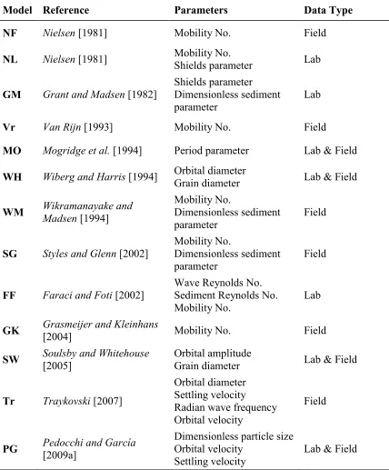
equilibrium models have been described in the literature. Table 1 shows the references of

13 most commonly used predictors spanning the years 1981 to 2009 as well as the type of

data they used for deriving their corresponding model.

The basis for many of the equilibrium ripple predictors is a set of dimensionless

parameters based on the flow properties and sediment characteristics. This approach was

first used by Yalin and Russell [1962] and further developed by others [Carstens et al., 1969; Mogridge and Kamphuis, 1972; Dinger, 1974; Pedocchi and García, 2009a]. The

parameters commonly include wave bottom orbital velocity (ub), wave period (T), median

sediment grain diameter (D50), sediment density (ρs), density of fluid (ρw), and gravity

(g). This has led to the development of the following non-dimensional parameters:





2 3

50 , b 50 , 1 50 , 1 ,

T  D u D  s gD  s 

 _{  } 

  _(2.1)

where s=ρs/ρw, ν is the kinematic viscosity of the fluid and ϕ is the angle of repose which

for sand is approximately equal to 32°. Various combinations of the above

non-dimensional numbers constitute the basis for many of the parameters commonly used in

sediment dynamics such as the mobility number, the wave Reynolds number, the

non-dimensional sediment parameter, the wave period parameter, and the ratio of the wave

orbital semi excursion to the sediment grain size (Ab/D50). A detailed description of the

derivation of these parameters can be found in Pedocchi and García [2009a] while the

corresponding equations are further described in section 2.2.

The plethora of equilibrium ripple predictors, the different scaling used between

them and the lack of agreement amongst them emphasizes the point that the problem has

used in the development of these models, with some of them being obtained in the field

and others in the laboratory; the quality of the data and the accuracy of the assumption

that the data used represent real equilibrium conditions.

Many of the early studies were primarily conducted in laboratory settings where

the hydrodynamics can be easily controlled and ripples consistently observed [e.g., Yalin

and Russell, 1962; Kennedy and Falcon, 1965; Carstens et al., 1969; Lofquist 1978). Later on, use of divers allowed for field observations under conditions conducive to the

diver’s safety and water visibility [e.g., Inman, 1957; Miller and Komar, 1980].

Subsequently, such observations were automated using underwater cameras which

allowed for regular sampling intervals but were hindered by reduced visibility during

energetic conditions [e.g., Boyd et al., 1988; Powell et al., 2000; Xu, 2005, and references

therein]. During the past two decades, the use of a stationary sector scanning sonar

system has allowed for continuous sampling during long deployments regardless of water

visibility [e.g., Hay and Wilson, 1994; Traykovski et al.,1999; Voulgaris and Morin,

2008; Warner et al., 2012] and wave activity levels. This proliferation of ripple

measurements and the collection of additional data allow for testing the performance of

existing models, their improvement, and possibly the development of a new model that

better predicts wave-induced ripples in the marine environment.

The objectives of this study are to: (i) assemble all existing data (field and

laboratory) of equilibrium ripples in a common database with commonly described

hydrodynamic forcing; (ii) enrich this database with additional information that has

is attempted by collecting existing data of ripple measurements from the published

literature as well as including data from two new field experiments. All data assembled

are presented in an electronic tabular form (see auxiliary material) for use by other

investigators and enrichment over time as new data become available.

The manuscript organization is so that section 2.2 presents a brief overview of the

most widely used equilibrium ripple predictors. This is followed with a presentation of

the ripple database and the source of the data (section 2.3). In section 2.4, an evaluation

of the existing predictors against all the data assembled is carried out, while a discussion

of their performance together with a new formulation is presented in section 2.5. Finally,

in section 2.6 the conclusions of the study are presented.

2.2. Existing Equilibrium Models

In this section, selective existing equilibrium models (see Table 2.1) are briefly

presented. The main criterion for their selection was their wide application in the

literature and their diversity in terms of forcing parameters used. All of the models

presented relate the ripple height and/or wavelength to hydrodynamic conditions usually

normalized by parameters describing the sedimentary particles. At this junction it should

be noted that different investigators have been defining the bottom orbital velocity

parameter differently depending on the method they used to make their estimates (i.e.,

from direct velocity time-series or wave height measurements) and the statistical

representation adopted. For example ub in Wikramanayake and Madsen [1994]

corresponds to standard deviation (σ) of oscillatory velocity, while in Grant and Madsen

[1982] and Styles and Glenn [2002] the same parameter corresponds to amplitude of

derived from significant wave height measurements correspond to 2∙σ [e.g., Traykovski et

al., 1999; Wiberg and Sherwood, 2008]. In order to avoid confusion, the parameters used

Table 2.1.Equilibrium ripple predictors examined in this study.

Model Reference Parameters Data Type

NF Nielsen [1981] Mobility No. Field

NL Nielsen [1981] Mobility No.

Shields parameter Lab

GM Grant and Madsen [1982] Shields parameter Dimensionless sediment parameter

Lab

Vr Van Rijn [1993] Mobility No. Field

MO Mogridge et al. [1994] Period parameter Lab & Field

WH Wiberg and Harris [1994] Orbital diameter

Grain diameter Lab & Field

WM Wikramanayake and _{Madsen [1994]}

Mobility No.

Dimensionless sediment

parameter Field

SG Styles and Glenn [2002]

Mobility No.

Dimensionless sediment parameter

Field

FF Faraci and Foti [2002]

Wave Reynolds No. Sediment Reynolds No.

Mobility No. Lab

GK Grasmeijer and Kleinhans _[2004] Mobility No. Field

SW Soulsby and Whitehouse _[2005] Orbital amplitude _{Grain diameter} Lab & Field

Tr Traykovski [2007]

Orbital diameter Settling velocity

Radian wave frequency Orbital velocity

Field

PG Pedocchi and García

Dimensionless particle size

through the adoption of appropriate subscripts are used that reveal the method of

estimation as well as the relationship between different parameters (see Table 2.2).

Table 2.2. Definitions and subscripts used for wave statistics.

Subscript Velocitya _{Wave height}

rms ub,rms=(σu2+σv2)1/2 0.5∙Hsig

eq(br) ub,eq=[2 ∙ (σu2+σv2)]1/2 Hrms=∙Hsig/√2

1/3 ub,1/3=2 ∙ (σu2+σv2)1/2 Hsig

1/10 ub,1/10=1.27 ∙ 2 ∙ (σu2+σv2)1/2 H1/10=1.27∙H1/3 a_σ

u2and σv2 denote variance of wave induced velocity.

In the remainder of this section, the existing equilibrium models are described in

sub-sections organized by the main parameter used in the model.

2.2.1. Mobility Number

One of the most common non-dimensional parameters used to determine ripple

geometry is the mobility number (ψ), which represents the ratio of mobilizing forces

acting on the sediment to the stabilizing forces:





2

50

1

b

u s g D

  _    _ (2.2)

where s is the normalized sediment density, g is the acceleration due to gravity and D50 is

the median particle size.

Nielsen [1981], proposed two sets of equations based on field/irregular and

laboratory/regular wave conditions denoted as NF and NL, respectively. The equations

developed for the regular monochromatic wave generated ripples were based on the

Mogridge and Kamphuis [1972], Dingler [1974], Nielsen [1979] and used laboratory data

from the Danish Hydraulic Institute. Nielsen [1981] found these ripples to be best

described by the equations:

,1/3 0.275 0.022 1/3 b

A

     (2.3)

0.34 ,1/3 2.2 0.345 1/3

b

A





where Ab is the wave orbital amplitude (=2π∙ub/T) and T is the wave period.

For field conditions, Nielsen [1981] used data collected from Inman [1957],

Dingler [1974], and Miller and Komar [1980] to propose the following set of equations:

1.85

,1/3 21 1/3 , 1/3 10

b

A







(2.5)



 



,1/3 693 0.37 1/3 1000 0.75 1/3

b

A exp ln ln

 _  _{ }  _{ }  

  (2.6)

For ψ1/3 < 10, Nielsen [1981] recommends using the ripple height from equation (2.3).

Nielsen [1981] also proposed a set of equations for ripple steepness based on the Shields

parameter, which is further discussed in section 2.3.

Van Rijn [1993] (Vr), also noted the potential scaling of ripple geometry with the

mobility number. He used ripple dimensions measured under irregular waves from Inman

[1957], Dingler [1974], Ribberink and Van Rijn [1987], Nieuwjaar and Van der Kaay

[1987] and Van Rijn [1987] and he suggested that equilibrium ripple geometry can be

predicted by:





0.22 , 10 2.8 10 250 , 1 0 250 b A             

 (2.7)

1/3 0.18 , 10



Grasmeijer and Kleinhans [2004] (GK) analyzed the ripple measurements of

Inman [1957], Van Rijn et al. [1993], Van Rijn and Havinga [1995], Grasmeijer and Van

Rijn [1999] and Hanes et al. [2001] as well as their own data collected off the coast of

Egmond aan Zee, Netherlands, and to suggest that:

0.5

1/3 1/3 ,1/3 1

1/3 1/3

0.275 0.022 , 10 2 , 10

b

A  



 

   

  _{ }

 (2.9)

1/3 0.221

1/3 1/3

0.14 , 10

0.078 0.355 , 10

        _{   }

 (2.10)

One commonality between the latter two models (i.e., Vr and GK) is that wave

steepness is assumed to be constant (0.14 and 0.18 for the GK and Vr models,

respectively) for low energy flows while it decreases under more energetic wave activity.

2.2.2. Mobility Number & Dimensionless Sediment Parameter

Another non-dimensional parameter used to determine ripple geometry is the ratio

of the mobility number (ψ) and the dimensionless sediment parameter (S*) with the latter

being defined as:

 

*

1

4

S



s

  

g D





This parameter was first proposed by Wikramanayake and Madsen [1994] and

later adopted by Styles and Glenn [2002]. In addition to taking into account the sediment

properties and orbital wave forcing, this parameter also accounts for water viscosity (ν)

and therefore requires knowledge of the water temperature, salinity and pressure (i.e.,

Wikramanayake and Madsen [1994] (WM) utilized the data from the field

measurements of Inman [1957], Miller and Komar [1980] and Nielsen [1984] and

suggested the following equations to predict ripple height and wavelength:









0.27 / , / 3

0.52 / , / 3

rms rms b rms rms rms S S A S S         _    

 (2.12)

and









1.70 / , / 3

2.10 / , / 3

rms rms b rms rms rms S S A S S         _    

 (2.13)

Equations (2.12) and (2.13) were later revised by Styles and Glenn [2002] (SG)

who incorporated additional field data from Wiberg and Harris [1994] and Traykovski et

al. [1999] to derive an improved fit between data and model so that:









0.30 / , / 2

0.48 / , / 2

eq eq b eq eq eq S S A S S         _       (2.14)









1.95 / , / 2

2.80 / , / 2

eq eq b eq eq eq S S A S S         _       (2.15)

where ψeq is the mobility number attained from calculating ub using the root mean square

(rms) wave height (or √2 times the variance of flow velocity). At this juncture, it should

be noted that equations (2.14) and (2.15) vary slightly from those in the original

manuscript of Styles and Glenn [2002] due to a typographical error in the original

manuscript [Styles, pers. comm.].

2.2.3. Shields Parameter Based Equilibrium Models

the wave Shields parameter (θ) [Shields, 1936]. For regular laboratory waves, Nielsen

[1981] suggested:

1.5 1/3

0.182 0.24

 









while for irregular field waves, he proposed:

4 1/3 0.342 0.34

     (2.17)

where θ is defined as:





2

50

0.5 f uw b s 1 g D

    _    _ (2.18)

with the wave friction coefficient (fw) defined as [Jonsson, 1966]:













0.194

50 50

50

5.213 2.5 / 5.977 , / 2.5 1.57

0.3 , / 2.5 1.57

b b

w

b

exp D A A D

f A D   _{  }  _{ }       

 _(2.19)

Grant and Madsen [1982] (GM) utilized data from Carstens et al. [1969] and found a relationship between the Shields parameter and ripple dimensions that defines

increasing ripple wavelengths with increasing Shields parameter value up to 1.8∙S*2 and

decreasing wavelengths thereafter. This led to a new set of equations for the prediction of

equilibrium ripples:









0.22 / , / 1.8

0.48 / , / 1.8

eq cr eq cr

b eq

eq cr eq cr

S A S S             _{  }        

 _(2.20)









0.16 / , / 1.8

0.28 / , / 1.8

eq cr eq cr

eq cr eq cr

S S S              _{  }        

 _(2.21)

2.2.4. Period Parameter

Mogridge et al. [1994] (MO) used the data of Bagnold [1946], Inman [1957],

Yalin and Russell [1962], Kennedy [1965], Horikawa [1967], Carstens et al. [1969], Mogridge [1972], Dingler [1974], Miller and Komar [1980], and Willis [1993] to

develop a set of equations that provide an upper limit on the ripple dimensions rather than

an actual prediction. These upper limits were related to a newly defined parameter χ as

follows:

0.03967 8.542 10.822 50 10

D 

 _  _(2.22)

0.02054

7

50 _{13.373 13.772 7} 1,394 , 1.5 10

10 , 1.5 10

D               

 _(2.23)

where χ relates sediment size to wave period as follows:





50

w D s g T

      (2.24)

While Nielsen [1981] argued that this parameter does not have any physical

meaning, Mogridge et al. [1994] suggested that the wave period directly reflects

velocities, accelerations, and forces of the oscillatory motion. Mogridge et al. [1994]

found η/D50 to be accurately described by a single equation; however, the ripple

wavelength diverges at χ values smaller than 1.5×10-5_{. They found that field data best}

conforms to a constant λ/D50 value of 1,394.

2.2.5. Orbital Excursion and Grain Size

Another parameter widely used to predict ripple dimensions is the wave orbital

excursion (do=2Ab) normalized by the sediment grain diameter (do/D50). Clifton [1976]

grain size (do /D50). For smaller values of do /D50, these orbital ripples have a wavelength

that scales with the wave orbital diameter.

Wiberg and Harris [1994] proposed a set of equations based on

orbital-suborbital-anorbital classification scheme using laboratory and field data from Inman [1957],

Kennedy and Falcon [1965], Carstens et al. [1969], Mogridge and Kamphuis [1972], and Dingler [1974]. The original Wiberg and Harris [1994] model requires an iterative

approach but Malarkey and Davies [2003] presented a modification that simplifies the

estimation of ripple characteristics:





,1/3 1 2 3 ,1/3

o o

d  exp C_  C C ln d  _

  _(2.25)





 

0.62 , / 20

0.62 0.01

535 , 20 / 100

535 5

535

o o ano

o

o ano

d d

d ln d

D exp ln d

D ln D                          

 , d_o,1/3/_ano 100

      _

 _(2.26)

where do,1/3/ηano is calculated using equation (2.25) with λ=λano=535∙D50, C1=7.59,

C2=33.60, C3=10.53, d o,1/3 is the significant wave orbital diameter, (ano) indicates the

anorbital ripple geometry and the equilibrium η is found using λ in equation (2.25).

Soulsby and Whitehouse [2005] (SW) used data from an extensive database of

published ripple dimensions, including the ones mentioned above, to suggest that scaling

of ripple geometry characteristics with the ratio of wave orbital semi-excursion of the

highest 1/10 velocities (Ab,1/10=1.27∙Ab,1/3) to the median particle diameter (D50) provides

the least scatter suggesting:









1.5

3 4

,1/10 1 1.87 10 ,1/10/ 50 1 2 10 ,1/10/ 50

b b b

A A D exp A D

     

 

 

 

 _        _









50 ,1/10

0.15 1 exp 5000 D A_b

    _  _

(2.28)

2.2.6. Orbital Excursion (do) and ws/ω

Similar to the predictors described above, Traykovski [2007] also noted that

ripples do tend to scale with orbital diameter. However, his predictor assumes that the

cutoff for orbital ripples (i.e., where ripples scale with the orbital diameter) occurs at a

value of ub,1/3/ws ≤ 4.2. Above this value, the ripples scale as a function of sediment

settling velocity (ws) and wave radian frequency (ω=2π/T). Traykovski [2007] found

strong agreement between ripples observed off the coast of Martha’s Vineyard

[Traykovski et al., 1999; Traykovski, 2007], using the following set of equations:

,1/3 ,1/3

,1/3

0.75 , / 4.2 6.3 / , / 4.2

o b s

s b s

d u w

w u w





 



  _{ }

 _(2.29)

where ws is the particle settling velocity calculated from Gibbs et al. [1971]. Assuming a

constant value for ripple steepness of η/λ = 0.16, the ripple equilibrium height is obtained

as:

,1/3 ,1/3

,1/3

0.12 , / 4.2 1.008 / , / 4.2

o b s

s b s

d u w

w u w





 



  _{ }

 _(2.30)

It is worth noting that according to equations (2.29) and (2.30), for ub,1/3/ws>4.2,

ripple geometry depends solely on wave period and sediment settling velocity. This

follows the observations of Mogridge et al. [1994] and might explain some of the scatter

and different trends observed in their predictor.

2.2.7. Reynolds Numbers

,1/3 ,1/3

w b b

Re



u



A



,1/3 50

d b

Re



u



D



Using ripple geometry data from wave tank experiments with both

monochromatic and irregular waves, they developed the following expressions for ripple

wavelength and height:

0.68 ,1/3 12.0613

b d w

A Re Re



(2.33)









,1/3 1 0.022 1 3 0.275 0.0076 0.1681

b w

A exp Re

 _{  } _ _{  } 

  _(2.34)

Although they found the measured ripple steepness to agree with Nielsen [1979],

they also noticed that the average steepness was 0.18, which corresponds to fully

developed vortex ripples. They suggested that ripple steepness must depend on the angle

of repose (ϕ) and recommended, as in Nielsen [1979, 1981], that:

0.32 tan

    (2.35)

which leads to η/λ=0.185 if an angle of repose of 30° is assumed.

2.2.8. Orbital Velocity / Settling Velocity

Pedocchi and García [2009a] used published ripple dimension data as well as

data from a wave tunnel experiment [Pedocchi and García, 2009b] to suggest that ripple

dimensions should be related to the ratio of ub,1/3/ws for three different grain size regimes

based on the particle Reynolds number (Rep). The latter relates to the dimensionless

particle size parameter (S*) as follows:





50 *

1 4

p

Re  s gD   S

(2.36)













0.65 0.050 / 1 , 13

0.65 0.040 / 1 , 9 13

0.65 0.054 / 1 , 9

b s p

b s p

b s p

u w Re

D u w Re

u w Re

     _{    }  _ _   _{ } _{ }   _     _{    }  _ _

 _(2.37)













0.1 0.055 / 1 , 13

0.1 0.055 / 1 , 9 13

0.1 0.055 / 1 , 9

b s p

b s p

b s p

u w Re

D u w Re

u w Re

     _{    }  _ _   _{ } _{ }   _     _{    }  _ _  (2.38)

where ws is the particle settling velocity calculated using the method of Dietrich (1982).

These equations are divided into three grain size regions with Rep=13 corresponding to

220 μm and Rep=9 corresponding to 177 μm at 20°C.

2.3. Data Availability

2.3.1. Existing Data Sources

Numerous experiments on oscillatory flow ripples have been carried out over the

years resulting in a large number of ripple wavelength and height data for a variety of

wave conditions and sediment sizes. Various subsets of these data were used in the

development of the equilibrium prediction models described in section 2.2. As part of this

study, all data available (see Table 2.3) are compiled into a single database to be used for

the production of a more comprehensive formulation for ripple equilibrium dimensions

that is not experiment or site specific. The ripple geometry data found in the literature

include descriptions of hydrodynamic forcing, sediment type and ripple dimensions;

orbital velocity (ub,1/3), wave period (T), median grain diameter (D50), water temperature

(Temp), water density (ρw), sediment density (ρs), water depth (h), salinity (S), ripple

wavelength (λ) and ripple height (η). For the experiments where wave forcing was listed

as wave height alone, the significant (1/3) bottom orbital velocity was calculated using

linear wave theory:

 

,1/3 1/3 2 sinh b

u H    _ kh _

(2.39)

where ω is the wave radial frequency, H1/3is the significant wave height, k is the

wavenumber, and h is the local water depth.

Another parameter, which is often omitted but required by several of the

predictors presented in section 2.2, is the water viscosity (ν). When water temperature,

salinity, and water depth data are provided, the viscosity is calculated from these values,

otherwise a water temperature of 20°C and a salinity of 0 is assumed for laboratory

experiments. For field experiments, temperature and salinity information obtained at a

nearby buoy from the national data buoy center (http://www.ndbc.noaa.gov/) is used.

When no historical data exist, an average (climatological) value of water temperature for

the specified month(s) of the experiment is taken and if no salinity is recorded, a value of

35 psu is assumed.

2.3.2. New Data Sources

In addition to the existing data described above, new data sets from two

experimental sites, representing different wave environments and sediment

characteristics, are also included in this database and subsequent analysis. Both sites are

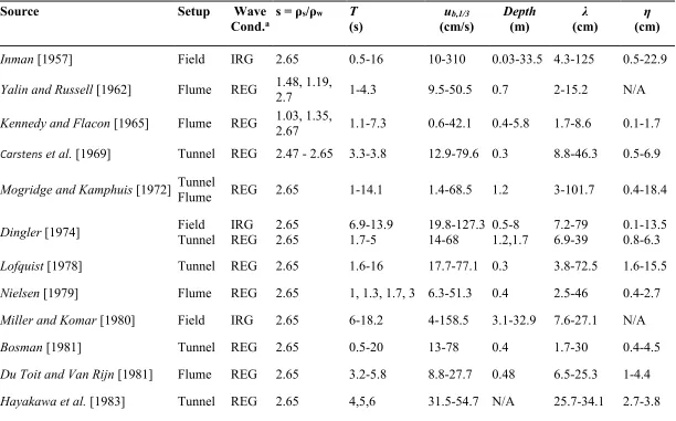
Table 2.3. Data sources used in this study.

Source Setup Wave

Cond.a

s = ρs/ρw T

(s) ub,1/3 (cm/s) Depth (m) λ (cm) η (cm)

Inman [1957] Field IRG 2.65 0.5-16 10-310 0.03-33.5 4.3-125 0.5-22.9

Yalin and Russell [1962] Flume REG 1.48, 1.19, _2.7 1-4.3 9.5-50.5 0.7 2-15.2 N/A

Kennedy and Flacon [1965] Flume REG 1.03, 1.35,

2.67 1.1-7.3 0.6-42.1 0.4-5.8 1.7-8.6 0.1-1.7

Carstens et al. [1969] Tunnel REG 2.47 - 2.65 3.3-3.8 12.9-79.6 0.3 8.8-46.3 0.5-6.9

Mogridge and Kamphuis [1972] Tunnel _Flume REG 2.65 1-14.1 1.4-68.5 1.2 3-101.7 0.4-18.4

Dingler [1974] Field Tunnel IRG REG 2.65 2.65 6.9-13.9 1.7-5 19.8-127.3 14-68 0.5-8 1.2,1.7 7.2-79 6.9-39 0.1-13.5 0.8-6.3

Lofquist [1978] Tunnel REG 2.65 1.6-16 17.7-77.1 0.3 3.8-72.5 1.6-15.5 Nielsen [1979] Flume REG 2.65 1, 1.3, 1.7, 3 6.3-51.3 0.4 2.5-46 0.4-2.7 Miller and Komar [1980] Field IRG 2.65 6-18.2 4-158.5 3.1-32.9 7.6-27.1 N/A Bosman [1981] Tunnel REG 2.65 0.5-20 13-78 0.4 1.7-30 0.4-4.5 Du Toit and Van Rijn [1981] Flume REG 2.65 3.2-5.8 8.8-27.7 0.48 6.5-25.3 1-4.4 Hayakawa et al. [1983] Tunnel REG 2.65 4,5,6 31.5-54.7 N/A 25.7-34.1 2.7-3.8

Nielsen [1984] Field IRG 2.65 5.3-14.4 39.1-113.6 0.8-1.8 5-150 0.5-20

Steetzel [1984] Tunnel REG

IRG 2.65 3-7 20-50 N/A 13-31.5 2-4.5

Sakakiyama et al. [1985] Flume REG 2.65 3-12 17-197 N/A 14.3-148 1.9-11.7 Nieuwjaar and van der Kaay

[1987] Tunnel IRG 2.65 2.4,2.5 21.2-47.6 N/A 8.5-9.3 1.1-1.8

Ribberink et al. [1987] Tunnel IRG 2.65 2-5 38.5-71.3 N/A 8-13.5 1-1.8 Boyd et al. [1988] Field IRG 2.65 3.1-11.4 6.4-121.6 9.6-12.5 7-24 N/A Van Rijn [1987] Tunnel IRG 2.65 4.6-6.3 62.2-178.2 N/A 20 0.1-2 Southard et al. [1990] Duct REG 2.65 3.1-19.3 10-100 0.2 12-196 2.1-23.9 Van Rijn [1993] Flume IRG 2.65 2.2-2.7 13.7-36.1 0.5 6-20 0.6-2.9 Ribberink and Al-Salem [1994] Tunnel REG 2.65 2-12 20-150 0.8 8.4-270 0.3-35

Van Rijn & Havinga [1995] Basin REG

IRG 2.65 2.1-2.3 14.4-29.9 0.4 5.9-11.1 0.6-1.4 Li & Amos [1998] Field IRG 2.65 8-12.8 1.9-28.8 38.7-40 7.7-15.4 0.8-2.2 Grasmeijer and Van Rijn [1999] Flume IRG 2.65 2.3 27-52.1 0.3-0.6 3.8-8.3 0.5-1.3 Hume et al. [1999] Field IRG 2.65 11 20-75 25 40-90 3-13 Traykovski et al. [1999] Field IRG 2.65 5.1-14.3 4.6-49.2 11.8-13.7 36.7-107 N/A Doucette [2000] Field IRG 2.65 4.7-12.2 17-102.8 0.3-1.7 5-70 0.5-11

Khelifa and Ouellet [2000] Basin REG 2.65 0.9-1.4 8.2-25.5 0.3 2.8-12.1 0.4-1.7 Williams et al. [2000] Flume REG 2.65 3.5-5 19-69 6.5 8-35 1.5-6 Faraci and Foti [2001] Flume REG

IRG 1.2, 2.65 1.3-4.2 5.4-86 0.2,0.3 3.7-12 0.4-2.1 Hanes et al. [2001] Field IRG 2.65 7.1-19.7 9.2-271.8 1.6-6.8 6-270 0.4-9.9 O’Donoghue and Clubb [2001] Tunnel REG

IRG

2.65 2-15 18-106 0.6 6-121

0.9-19.4 Ardhuin et al. [2002] Field IRG 2.65 11.4-13.8 37-67

19.7-27.6 77-137 N/A Doucette [2002] Field IRG 2.65 2.2-12.2 15.6-59.1 0.2-1.1 8-91 2-14 Faraci and Foti [2002] Flume REG

IRG 2.65 1.3-4.2 12.7-35 0.3 4.4-10.7 0.7-2.1 Sleath and Walbridge [2002] Tunnel REG 2.65 2.8-6.8 8-164 0.3 10-50 1.7-9 Thorne et al. [2002] Flume IRG 2.65 4-6 25.7-65.8 4.5 26.2-51.3 4-6.5 Grasmeijer and Kleinhans [2004] Field IRG 2.65 4-10.5 23-98.5 2 19-200 0.7-10 Williams et al. [2004] Flume IRG 2.65 4-6

13.1-102.6

4,4.5 20-104 1-7

Dumas et al. [2005] Tunnel REG 2.65 7.9-11

20.1-165.3 0.7 6.5-723.8 0.4-53.2 Smith & Sleath [2005] Tray REG 2.65 0.9-3.8 15.6-49 0.4 3.5-30.7 0.3-4.1 Xu [2005] Field IRG 2.65 8.8-18.3 15.6-43.8 15 4.6-7.5 N/A Brown [2006] Flume REG

IRG

2.65 4,6,8 26.5-66.8 4.6 5.5-23 0.2-2.3

Doucette and O’Donoghue [2006] Tunnel REG _IRG 2.65 2-12.5 29.8-146.6 0.5 8.7-82.3 1.3-12.8

O’Donoghue et al. [2006] Tunnel REG

IRG 2.65 3.1-12.5 27-88 0.5,0.8 11.4-110.7 1.5-13.9 Traykovski [2007]

Martha's Vineyard Coastal Observatory 2002 2005 Field Field IRG IRG 2.65 2.65 1-12.9 6.2-11.6 5.5-133.1 12-80.9 12-13.9 12.3-13.7 10-127 39.4-127.8 N/A 2.9-16.6

Pedocchi and García[2009b] Tunnel REG 2.65 2-25 20-100 0.6 5-180 0.6-19 This Study

Long Bay, SC Georgia Shelf Field Field IRG IRG 2.65 2.65 4.8-12.7 6.5-12.3 6.6-43.9 3.1-45.6 8.2-10.6 26.1-29 7-22.4 9.5-75.8 N/A N/A

a_{REG (IRG) denote regular (irregular) wave conditions.}

respectively. The first field data set is from the shelf on the northern part of South

Carolina (USA) off Long Bay (33° 43.35’N, 78° 46.75’W) (Figure 2.1). These data were

collected as part of the U.S. Geological Survey’s South Carolina Coastal Erosion Study,

which took place from October 2003 to April 2004 [Sullivan et al., 2006; Schwab et al.,

2009; Warner et al., 2012]. The seabed sediment at this site consists of fine to medium

quartz sand with a median grain diameter (D50) of 177 μm. Data from the period 30

January 2004 to 15 March 2004 is used in this study as this provides the most complete

record of hydrodynamic and bedform wavelength data. The second data set is from the

continental shelf off the coast of Georgia, USA (31° 22.343’N, 80° 34.073’W) (Figure

2.2). The seabed at this site consists of medium to coarse sand with a mean diameter of

388 μm. Two periods of simultaneous hydrodynamic and bedform imagery data

collection is used, corresponding to 16 September 2007 to 7 October 2007 and 13

December 2007 to 15 February 2008. These periods include several sediment

mobilization events where bedforms change dimension and orientation (Figure 2.2). The

detailed description of the experimental setup, hydrodynamic conditions, ripple evolution

description as well as the methodologies used are presented in detail in chapter 3 and in

Voulgaris and Morin [2008]. It should be noted that these data sets do not contain any

ripple height observations and are limited to wavelength information only.

2.3.3. Equilibrium Ripple Criterion

Some of the data sources contain measurements of mega ripples with wavelengths

of up to 8 m; since this study focuses on wave ripples only, any ripples with wavelengths

Figure 2.1. Time series of data collected in Long Bay, South Carolina (USA) during 2004: (a) significant wave orbital velocity (black) and wave period (gray); (b) wave Shields parameter (black) and critical Shields parameter (gray); (c) measured ripple wavelength. The shaded areas indicate periods when 0<dθ/dt<0.1∙θ1/3 (t)/Tk(t) and

θ1/3>1.5θcr (see text).

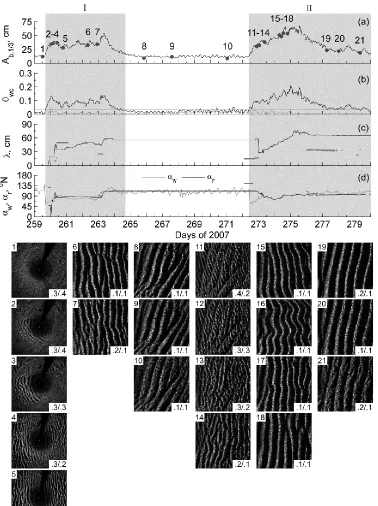
Figure 2.2. Time series of data collected in the South Atlantic Bight off Georgia (USA) during 2007-2008: (a) significant wave orbital velocity (black) and wave period (gray); (b) wave Shields parameter (black) and critical Shields parameter (gray); and (c) measured ripple wavelength. The shaded areas indicate periods when

0<dθ/dt<0.1∙θ1/3 (t)/Tk(t) andθ1/3>1.5θcr (see text).

experiments carried out at high water temperature (~60°C) [e.g., Southard et al., 1990;

Dumas et al., 2005]. The following criteria were used to ensure that the data used

represent equilibrium conditions with the flow. Since laboratory experiments are run until

Shields parameter greater than the critical Shields parameter for sediment motion

(θ1/3>θcr), is assumed to represent ripples in equilibrium with the flow. For field

conditions, where an objective definition of equilibrium is difficult without information

of the time history of the ripple evolution, only ripple data corresponding to θ1/3>2∙θcr are

considered to be in equilibrium. For the cases where time history of the ripple evolution

is known (Traykovski et al. [1999], Traykovski [2007] and the data discussed in section

2.3.2), equilibrium ripples were identified as those recorded during periods where the

hydrodynamic forcing (i.e., excess Shields parameter) does not change significantly over

the time required for a ripple to adjust itself to the given hydrodynamic forcing. This

corresponds to the time scale (Tk) given in Traykovski [2007, equation (9)] and it is a

function of the Shields parameter (θ1/3). Thus only ripple data corresponding to

conditions where 0<dθ1/3/dt<0.1∙θ1/3(t)/Tk(t) are assumed to be in equilibrium with the

flow. A further criterion of θ1/3>1.5∙θcr was applied to eliminated low energy conditions

where the bed may only experience intermittent sediment mobilization during a wave

group and hence would require more time than what the time scale Tk predicts.

The database developed from all sources of data described in the previous two

sections includes ripple data from experiments conducted with both

regular/monochromatic waves and irregular/random waves, with the former consisting of

data from laboratory experiments only. After applying the wavelength and equilibrium

criteria, the regular wave data set left consists of 1,145 measurements of wavelength and

1,049 measurements of ripple steepness. The irregular wave data set consists of all field

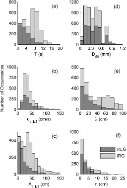
dimensions (height and wavelength), hydrodynamic conditions (wave period, orbital

velocity and bottom excursion), and grain sizes incorporated in this data set are shown in

Figure 2.3. The combination of regular and irregular wave data results in a total of 2,910

measurements of ripple wavelength and 1,748 measurements of ripple steepness.

Figure 2.3. Frequency distribution of range of values for parameters representing hydrodynamic forcing and ripple dimensions for the ripple data sets compiled for this study (N=2,968). Data

2.4. Results

In this section, all previously published and the newly collected data that have

passed the equilibrium criteria are used to evaluate the predictors presented in section 2.2.

2.4.1. Mobility Number based Equilibrium Models

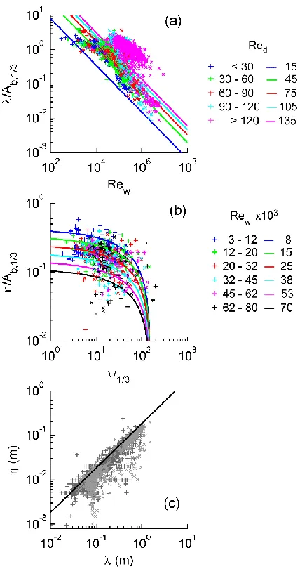
The predictions of equilibrium ripple length, height and steepness using the

mobility number based models (i.e., NF, NL, Vr and GK) are plotted against the

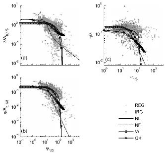
observations in Figure 2.4. All ripple dimensions have been normalized by the bottom

orbital semi-excursion (Ab,1/3).

It is worth noting that all four models converge for ψ1/3 < 10 predicting a nearly

constant value indicating a sole dependence of ripple dimensions on Ab. However, this

trend is not supported by the data, which show a gradually increasing λ/Ab ratio for

decreasing ψ1/3. The ripple wavelength data (see Figure 2.4a) suggests either an inverse

relationship between normalized wavelength and ψ1/3 or a constant value that should be

larger than that predicted by these models. For ψ1/3 > 10, the models start deviating from

each other with the irregular wave data suggesting two trends. One trend follows the

predictors of NL, Vr, and to an extent, that of GK while the remaining data follow that of

NF and yield a smaller λ/Ab,1/3 ratio value for the same ψ1/3. This deviation was also noted

by Nielsen [1981], who attributed it to differences between laboratory/regular vs.

field/irregular waves. However, this is not the case in here, as ripples under different

wave forcing appear to follow either trend without a specific reference to

regular/irregular forcing or sediment size.