An Earley Type Parsing Algorithm for Tree Adjoining Grammars

(1)

A N E A R . L E Y - T Y P E P A R . S I N G A L G O R . I T H M

F O R . T R . E E A D J O I N I N G

G R _ k M M A R . S

*

Y v e s S c h a b e s a n d A r a v i n d K . J o s h i

Department of Computer and Information Science University of Pennsylvania

Philadelphia PA 19104-6389 USA

schabes~liac.cis.upenn.edu joshi~cis.upenn.edu

A B S T R . A C T

We will describe an Earley-type parser for Tree Adjoining G r a m m a r s (TAGs). Although a CKY- type parser for TAGs has been developed earlier (Vijay-Shanker and :Icshi, 1985), this i s the first practical parser for TAGs because as is well known for CFGs, the average behavior of Earley-type parsers is superior to t h a t of CKY-type parsers. The core of the algorithm is described. Then we discuss modifications of the parsing algorithm t h a t can parse extensions of TAGs such as constraints on adjunction, substitution, and feature structures for TAGs. We show how with the use of substitution in TAGs the system is able to parse directly C F G s and TAGs. T h e system parses unification formalisms t h a t have a C F G skeleton and also those with a T A G skeleton. Thus it also allows us to embed the essential aspects of PATR-II.

1

I n t r o d u c t i o n

Although formal properties of Tree Adjoining G r a m m a r s (TAGs) have been investigated (Vijay- Shanker, 1987)--for example, there is an

O(ns)-

time CKY-like algorithm for TAGs (Vijay-Shanker and Joshi, 1985)--so far there has been no at- t e m p t to develop an Earley-type parser for TAGs. This paper presents an Earley parser for TAGs and discusses modifications to the parsing algorithm t h a t make it possible to handle extensions of TAGs such as constraints on adjunction, sub-

*This work i s partially supported by ARO grant DAA29-84-9-007, DARPA grant N0014-85-K0018, NSF grants MCS-82-191169 and DCR-84-10413. The authors would like to express their gratitude to Vijay-Shankc~r for his helpful comments relating to the core of the algorithm, Richard Billington and Andrew Chalnlck for their graphi- cal TAG editor which we integrated in our system and for their programming advice. Tb,m~ are also due to Anne Abeill~ and Ellen Hays.

stitution, and feature structure representation for TAGs.

TAGs were first introduced by Joshi, Levy and Takahashi (1975) and Joshi (1983). We describe very briefly the Tree Adjoining G r a m m a r formal- ism. For more details we refer the reader to Joshi (1983), Kroch and Joshi (1985) or Vijay-Shanker

(1987).

D e f i n i t i o n 1 ( T r e e A d j o i n i n g G r a m m a r ) : A TAG is a 5-tuple

G -- (VN, VT,S,I,A)

where

VN

is a finite set of non-terminal symbols,

VT

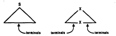
is a finite set of terminals, S is a distinguished non- terminal, I is a finite set of trees called i n i t i a l t r e e s and A is a finite set of trees called a u x i l i a r y t r e e s . T h e trees in I U A are called e l e m e n t a r y t r e e s .

I n i t i a l t r e e s (see left tree in Figure 1) are characterized as follows: internal nodes are labeled by non-terminals; leaf nodes are labeled by either terminal symbols or the empty string.

S

Li~minill$

x

/ x \

tofnflnld$

J

Ltef rntnll|$

Figure h Schematic initial and auxiliary trees

A u x i l i a r y t r e e s (see right tree in Figure 1) are characterized as follows: internal nodes are labeled by non-terminals; leaf nodes are labeled by a terminal or by the e m p t y string except for exactly o n e node (called the f o o t n o d e ) labeled by a non-terminal; furthermore the label of the foot node is the same as the label of the root node.

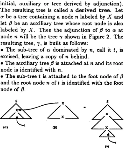
[image:1.612.323.519.485.546.2]

(2)

initial, auxiliary or tree derived by adjunction). The resulting tree is called a d e r i v e d t r e e . Let c~ be a tree containing a node n labeled by X and let fl be an auxiliary tree whose root node is also labeled by X. Then the adjunction of fl to a at node n will be the tree 7 shown in Figure 2. The resulting tree, 7, is built as follows:

* The sub-tree of a dominated by n, call it t, is excised, leaving a copy of n behind.

• The auxiliary tree fl is attached at n and its root node is identified with n.

• The sub-tree t is attached to the foot node of # and the root node n of t is identified with the foot node of ft.

$

%,

(ct} (1~)

$

Figure 2: The mechanism of adjunction

Then define the t r e e s e t of a TAG G,

T(G)

to be the set of all derived trees starting from initial trees in I. Furthermore, the s t r i n g l a n g u a g e generated by a TAG, L(G), is defined to be the set of all terminal strings of the trees in

T(G).

TAGs factor recursion and dependencies by ex- tending the domain of locality. They offer novel ways to encode the syntax of natural language grammars as discussed in Kroch and Joshi (1985) and Abeill~ (1988).

In 1985, Vijay-Shanker and Joshi introduced a CKY-like algorithm for TAGs. They therefore es-

tablished

O(n 6)

time as an upper bound for pars-

ing TAGs. The algorithm was implemented, but in our opinion the result was more theoretical than practical for several reasons. First the algorithm assumes that elementary trees are binary branch- ing and that there are no empty categories on the frontiers of the elementary trees. Second, since it works on nodes that have been isolated from the tree they belong to, it isolates them from their domain of locality. However all important linguistic and computational properties of TAGs follow from this extended domain of locality. And most

importantly, although it runs in

O(n 6)

worst time,

it also runs in

O(n s)

best time. As a consequence,

the CKY algorithm is in practice very slow. Since the average time complexity of Earley's parser depends on the grammar and in practice

runs much better than its worst time complexity, we decided to try to adapt Earley's parser for CFGs to TAGs. Earley's algorithm for CFGs (Earley, 1970, Aho and Ullman, 1973) is a bottom- up parser which uses top-down information. It manipulates states of the form A -* a.fl[i] while using three processors: the predictor, the comple- tot and the scanner. The algorithm for CFGs runs in

O(IGl2n s)

time and in

O(IGI n2)

space in all cases, and parses unambiguous grammars in O(n 2) time (n being the length of the input, IGI the size of the grammar).

Given a context-free grammar in any form and an input string al " ' a n , Earley's parser for CFGs maintains the following invariant:

The state

A --* a./3[i]

is in states set Skiff

S ::b 6A'r, 6 : b a l " "ai and a ~ ai+l ""ak

The correctness of the algorithm is a corollary of this invariant.

Finding a Earley-type parser for TAGs was a difficult task because it was not clear how to parse TAGs bottom up using top-down information while scanning the input string from left to right. In order to construct an Earley-type parser for TAGs, we will extend the notions of dotted rules and states to trees. Anticipating the proof of correctness and soundness of our algorithm, we will state an invariant similar to Earley's original invariant. Then we present the algorithm and its main extensions.

2

D o t t e d

s y m b o l s ,

d o t t e d

t r e e s , t r e e t r a v e r s a l

The full algorithm is explained in the next section. This section introduces preliminary concepts that will be used by the algorithm. We first show how dotted rules can be extended to trees. Then we introduce a tree traversal that the algorithm will mimic in order to scan the input from left to right. We define a d o t t e d s y m b o l as a symbol asso-

ciated with a dot

above

or

below

and either to

the

left

or to

the right

of it. The four positions of the

dot are annotated by

In, lb, ra, rb

(resp. left above,

left below, right above, right below): laura l b ~ r b • Then we define a d o t t e d t r e e as a tree with exactly one dotted symbol.

[image:2.612.81.298.91.351.2]

(3)

START "'~ f END

i'A,; o

E F G H I

2.1 2.2 2.3 &1 3.2

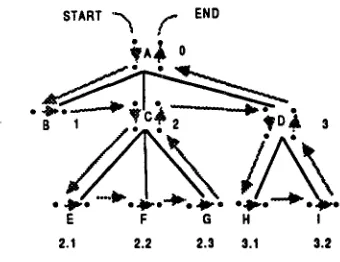
Figure 3: Example of a tree traversal

• if t h e dot is at position la of an internal node, we move the d o t down to position lb,

• if the dot is at position lb of an internal node, we move t o position la o f its leftmost child, • if the dot is a t position la o f a leaf, we move the dot to the right to position ra of the leaf,

• if the dot is at position rb of a node, we move

the dot up to position ra of the same node,

• if the dot is at position ra of a node, there are

t w o cases:

- if the node has a right sibling, then move the dot to the right sibling at position la.

- if the node does not have a right sibling, then move the dot to its parent at position rb.

This traversal will enable us to scan the frontier of an elementary tree from left to right while try- ing to recognize possible adjunctions between the above and below positions of the dot.

3

T h e a l g o r i t h m

We define an appropriate d a t a structure for the algorithm. We explain how to interpret the structures t h a t the parser produces. T h e n we describe the algorithm itself.

3.1

D a t a s t r u c t u r e s

T h e algorithm uses two basic d a t a structures: state and states set.

A s t a t e s s e t S is defined as a set of states. T h e states sets will be indexed by an integer: Si with i E N . T h e presence of any state in states set i will m e a n t h a t t h e input string al...al has been recognized.

A n y tree ~ will be considered as a function from tree addresses to symbols of the g r a m m a r (terminal and non-terminal symbols): if z is a valid address in a, then a ( z ) is the symbol at address z

in the tree a.

D e f i n i t i o n 2 A s t a t e s is defined as a 10-tuple,

[a, dot, side,pos, l, ft, fr, star, t~, b~] where: • a: is the name of the d o t t e d tree.

• dot: is the address of the dot in the tree a.

• side: is the side of the symbol the dot is on;

side E {left, right}. • pos: is the position of the dot;

pos E {above, below}.

• star. is an address in a. T h e corresponding node in a is called the starred node.

• ! (left), ft (foot left), f r (foot right), t~ (top left of starred node), b~ ( b o t t o m left of starred node) are indices of positions in the input string ranging over [O,n], n being the length of the input string. T h e y will be explained further below.

3.2

I n v a r i a n t o f t h e a l g o r i t h m

T h e states s in a states set Si have a c o m m o n prop- erty. T h e following section describes this invariant in order to give an intuitive interpretation of what the algorithm does. This invariant is similar to Earley's invariant.

Before explaining the main characterization of the algorithm, we need to define the set of nodes on which an adjunction is allowed for a given state.

D e f i n i t i o n 3 T h e set of nodes 7~(s) on which an adjunction is possible for a given state

s - [a, dot, side, pos, l, f h f i , s t a r , t~,b~], is defined as t h e union of t h e following sets of nodes in a :

• the set of nodes t h a t have been traversed on the left and right sides, i.e., the four positions of the dot have been traversed;

• the set of nodes on the p a t h from t h e root node to the starred node, root node and starred node included. Note t h a t if there is no star this set is empty.

D e f i n i t i o n 4 ( L e f t p a r t o f a d o t t e d t r e e ) T h e left part of a d o t t e d tree is the union of the set of nodes in the tree t h a t have been traversed on the left and right sides and the set of nodes t h a t have been traversed on the left side only.

We will first give an intuitive interpretation of the ten c o m p o n e n t s of a state, and then give the necessary and sufficient conditions for membership of a state in a states set.

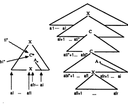
We interpret informally a state

[image:3.612.78.248.77.208.2]

(4)

"' 7

C ~

^"

Tit!,

_al _... _all _atl+l _.... _ah'

Figure 4: Meaning of s E Si

• l is an index in the input string indicating where the tree derived from a begins.

• ft is an index in the input string corresponding to the point just before the foot node (if any) in the tree derived from a.

• f i is an index in the input string corresponding to the point just after the foot node (if any) in the tree derived from a . T h e pair fi and f i will mean t h a t the foot node subsumes the string al,+,...ay,.

• star:, is the address in a of the deepest node that subsumes the dot on which an adjunction has been partially recognized. If there is no adjunction in the tree a along the path from the root to the dotted node, star is unbound.

• t~ is an index in the input string corresponding to the point in the tree where the adjunction on the starred node was m a d e . If star is unbound, then t~ is also unbound.

• b~ is an index in the input string corresponding to the point in the tree just before the foot node of the tree adjoined at the starred node. The pair t~ and b~ will mean t h a t the string as far as the foot node of the auxiliary tree adjoined at the starred node matches the substring alT+l...ab7 of the input string. If star is unbound, then b~ is also unbound.

• s E Si means that the recognized part of the dotted tree a, which is the left part of it, is consistent with the input string from al to aa and from at to aI, and from ay. to ai, or from a I to al and from az to al when the foot node is not in the recognized part of the tree.

We are now ready to characterize the membership of s in S~:

I n v a r i a n t 1

A state s = [a, dot, side,pos, l, f h fr, star, t~, b~] is in Si if and only if there is a derived tree from an initial tree such that (see Figure 4):

1. The tree a is part of the derivation.

2. The tree derived from a in the derivation tree, ~, has adjunctions only on nodes in 7~(s). 3. The part of the tree to the left of the dot in the tree derived spans the string al ... ai.

4. The tree derived from a, E, has a yield that starts just after ah ends at ay, before the foot node (if ay, is defined), and starts after the foot node just after ay, (if aI, is defined).

5. If there are adjunctions on the path from the dotted node to the root of a, then star is the address of the deepest adjunction on that path and the auxiliary tree adjoined at that node star has a yield that starts just after a,~ and stops at its foot node at ab t.

T h e proof of this invariant has as corollaries the soundness, completeness, and therefore the correctness of the algorithm.

3 . 3 T h e r e c o g n i z e r

The Earley-type recognizer for TAGs follows:

Let G be a TAG.

Let al...a, be the input string.

program recognizer

b e g ~

So = { [a, O,

left,

above, 0

. . . -] ]a is an initial tree } F o r i := 0 t o n d o

begin

Process the states of S i , performing one of

the f o l l o w i n g s e v e n o p e r a t i o n s on each state

s = [c~, dot, side,pos, l, f,, fr, star, t~, b~]

until no m o r e states can be added: I. S c - ~ e r

2. M o v e dot d o w n

S . M o v e d o t up

4. Left Predictor 5. Left Completor 6. Right Predictor 7. Right Completor

If Si+1 is empty and i < n, return rejection.

e n ~

If there is in S. a state

s = [ a , O , right, above,O . . . . , - ]

such that ~ is an initial tree then return acceptance.

[image:4.612.64.280.75.256.2]

(5)

T h e algorithm is a general recognizer for TAGs. Unlike the C K Y algorithm, it requires no condi- tion on the g r a m m a r : the trees can be binary or not, the elementary (initial or auxiliary) trees can have the e m p t y string as frontier. It is an off-line algorithm: it needs to know the length n of the input string. However we will see later t h a t it can very easily be modified to an on-line algorithm by the use of an end-marker in the input string.

We now describe one by one the seven processes. T h e current states set is presumed to be S / a n d the state to be processed is

s = [a, dot, side, pos, l, fZ, fr, star, tT].

Only one of the seven processes can be applied

to a given state. T h e side, the position, and the

address of the dot determine the unique process

that can be applied to the given state.

D e f i n i t i o n 5

(Adjunct(a, address))

Given

a T A G G, define

Adjunct(a, address) as

the set

of auxiliary trees t h a t can be adjoined in the ele- m e n t a r y tree ct at t h e node n which has the given address. In a T A G w i t h o u t any constraints on adjunction, if n is a non-terminal node, this set consists of all auxiliary trees t h a t are rooted by a node with same label as t h e label of n.

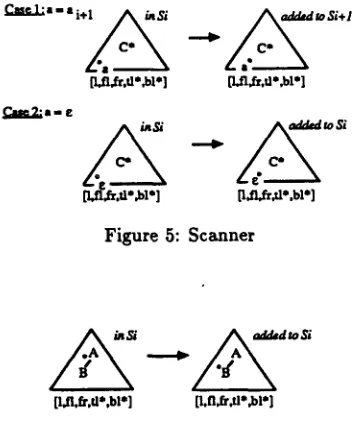
3 . 3 . 1 S c a n n e r

T h e scanner scans the input string. Suppose t h a t the dot is to t h e left of and above a terminal symbol (see Figure 5). T h e n if the terminal symbol matches the next input token, the p r o g r a m should record t h a t a new token has been recognized and try to recognize the rest of the tree.

Therefore "the scanner applies to

s = [a, dot, left, above, 1, ft, L , star, t[, b[]

s u c h t h a t

,',(dot)

i s a t e r m i n a l symbol and

~(dot)

= ~ + I or

~(dot)

is the empey symbol

• Case 1: a ( d o t ) = ai+l

The s c a n n e r adds

[~, dot, right, above, 1, f,, f i , star, t[ , b[ ] "co

SI+I

•

• Case 2:

a(dot)

=

The s c a n n e r adds

[tr, dot, right, above, l, ft, fr, star, t[ , b[ ] t o

S,.

3.3.2 - M o v e D o t D o w n

Move dot down (See Figure 6), moves the dot down, f r o m position

lb

of the d o t t e d node to posi-

C~e 1:a = a i ÷ ~

[1£1/T, tl*~l*]

C ~ l e 2." i m E

~toSi+l

[1~1~,d',b1"]

Bjl~,tl'.bl']

Figure 5: Scanner

[l,fl,fr,tl*,bi*]

[l.flJr,tl*~ol*]

Figure 6: Move dot down

tion

la

of its leftmost child.

It t h e r e f o r e applies ¢o

s = [~, d ~ , left, below, l, ~ , f , , star, t[, b[]

s u c h t h a t ~ h e n o d e w h e r e t h e d o ~ i s h a s a l e f ~ m o s t c h i l d a t a d d r e s s u .

I t a d d s [a, u,

left, above, I, ~ , re, star, t[ , b~ ] t o

S,.

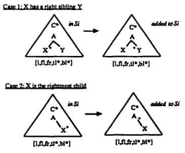
3 . 3 . 3 M o v e D o t U p

Move dot up (See Figure 7), moves the dot "up", f r o m position

ra

of the d o t t e d node to position

la

of its right sibling if it has a right sibling, other- wise to position

rb

of its parent.

It therefore applies to

s = [a,

dot, ~ g h t , above, l, ~, f i , star, t[, b[]

s u c h t h a t t h e n o d e on which t h e d o t i s h a s a p a r e n t n o d e .

• Case 1: the node where the dot is

has a right sibling at address r.

I t adds

[ct, r, left, above, l, fz, fr, star, t~ , b~]

~o S,.

• Case 2 : t h e node w h e r e t h e d o t i s i s

~he rightmost child of the parent

node p .

It a d d s

[image:5.612.328.505.78.290.2]

(6)

[l~lJr, tl*,bl*]

a d d ~ m S /

[l,fl,f~',tl *,bl*]

Clme 92 X ii thv r l o h l r n ~ child

[image:6.612.59.544.59.734.2] [image:6.612.75.258.80.232.2]

[l.fl,fi',tl',bl'] [l.fl,fr, tl*.bl']

Figure 7: M o v e dot up

3 . 3 . 4 L e f t P r e d i c t o r

Suppose t h a t there is a dot to the left of and above a non-terminal symbol A (see Figure 8). T h e n the algorithm takes two paths in parallel: it makes a prediction of adjunction on the node labeled by A and tries to recognize the adjunction (stepl) and it also considers the case where no adjunction has been done (step2). These operations are performed by the L e f t P r e d i c t o r .

It applies t o

s = [~, dot, left, above, 1, h , fr, aar, t~, b~]

such that

~(dot)

is a non-terminal.

• S t e p I. It adds the states

(LS,0,1eft, above, i . . .

-]

[B E A d j u n a ( ~ , dot) } t o Si.

• S t e p 2.

- - Case 1: t h e d o t is n o t on t h e f o o t n o d e .

I t adds t h e s t a t e

[~, dot, left, below, 1, ~ , fi , star, t~ , b~ ]

t o

S,.

- - Case 2: t h e d o t i s on t h e f o o t n o d e . N e c e s s a r i l y , s i n c e t h e f o o t node h a s n o t b e e n a l r e a d y t r a v e r s e d , ~ and

fr

are

unspecified. It adds the state

[~, dot, left, below, l, i, - , star, t~ , b~ ] t o

S,.

3.3.5 L e f t C o m p l e t e r

Suppose t h a t the auxiliary t h a t we left-predicted has been recognized as far as its foot (see Fig- ure 9). T h e n the algorithm should try to recognize

[I. n. fr. tl.. bl.] ~, (i.-.-.-.-] J

[1, fl, fr, tl" ,bl*] [1, ft. fr, tl", bl*]

£---'A

[l.-.-.tl-~l.] [ki.-.tt.~l']

Figure 8: Left Predictor

[ r , f l ' , f r ' , t l * ' , b l * ' ]

[l.i.-.tl*,bl*] [ r , f l ' , f r ' , l . i ]

Figure 9: Left completer

w h a t was pushed under the foot node. (A star in the original tree will signal t h a t an adjunction has been made and half recognized.) This operation is performed by the L e f t C o m p l e t e r .

It applies to

s = [a, dot, left, below, l, i, - , star, t~, b~]

s u c h t h a t t h e d o t i s on t h e f o o t n o d e . F o r a l l

I I I t I ,n St

s = L 8, dot , left, above, l , f;, f~, s t a r ,

t t , bt ] i n Sz s u c h t h a t a E

Adjunct(B, dot')

Case I: dot' is on the foot node of B. Then necessary, f[ a n d f~ are unbound.

LS, dot',left, below, l ' , i , - , d o t ' , l , ~

to S,.

Case 2: dot ~ i s n o t on t h e f o o t node o f

B.

(7)

Case l

[tl*,bl*,-,tl*',bl*']

~ * ~ 1 " 1

/--.--. A .=..=~ [tI* ,bl" ,l,tl*',bl*']

Case 2

aldd to~Z.

[image:7.612.44.532.69.663.2]

p.~.tl*.bl*]

Figure I0: Right Predictor

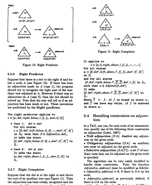
3 . 3 . 6 R i g h t P r e d i c t o r

Suppose that there is a dot to the right of and below a node A (see Figure I0). If there has been an adjunction m a d e on A (case I), the program should try to recognize the right part of the auxiliary tree adjoined at A. However if there was no adjunction on A (case 2), then the dot should be moved up. Note that the star will tell us if an adjunction has been m a d e or not. These operations are performed by the Right predictor.

The r i g h t p r e d i c t o r a p p l i e s t o

s = [a, dot, right, below, l, fz, fr, star, tT, bT]

• Case 1:

dot = star

For all s t a t e s

, t $;

s = [/3, dot', left, below, t~, bT, - , star ~-, t t , b t ].

in

Sb 7

s u c h t h a t ~ ¢

A d j u n c t ( a , dot),

i t a d d s t h e s t a t e

L O, dot', right, below,tT, * "

bz , , , s t a r ' , t z ,b I ] t o

*' *'

s,.

• C a s e 2:

dot ~ star

It a d d s t h e s t a t e

[a,

dot, right, above, l, fl, fr, star, tT , bT ] t o

S,.

3.3.7 R i g h t C o m p l e t o r

Suppose that the dot is to the right ot and above the root of an auxiliary tree (see Figure 11). Then the adjunction has been totally recognized and the program should try to recognize the rest of the tree in which the auxiliary tree has been adjoined. This operation is performed by the Right Completor.

[l',fl',fr',tl *'.bl *']

[I,fl,t~e,-I

~ a d d t d to$i

[l',.~',~'r',tl*'.bl *']

Figure 11: Right C o m p l e t o r

It applies t o

s = [a, 0,

right, above, l,

fz, L, -, -, -]

F o r all states

s!

=

[/3,

dot',

left, above,

l',

f[ ,

fir,

star',

t~', b~']

inS,

and for all states

LS,

dot',right,

below,

t',T,,~,dot',Z,

fd in aS,

such that a E

Adjunct(E,

dot')

I t adds

Lff , dot', right, above, l',-~l , 7~r, star', t;', 6;']

to

S,.

N h e r e 7 = f , i f f i s bound i n s t a t e s t , and f c a n h a v e a n y v a l u e , i f f i s unbound i n s t a t e e l .

3.4

H a n d l i n g c o n s t r a i n t s on adjunc-

tion

In a T A G , one can, for each node of an elementary tree, specify one of the following three constraints on adjunction (Joshi, 1987):

• Null adjunction (NA): disallow any adjunction on the given node.

• Obligatory adjunction (OA): an auxiliary tree must be adjoined on the given node.

• Selective adjunction

(SA(T)): a set T

of auxiliary trees that can be adjoined on the given node is specified.

T h e algorithm can be very easily modified to handle those constraints. First, the function

A d j u n c t ( a , address)

m u s t be modified as follows:

• A d j u n c t ( a , address)

= ~, if there is

N A

on the

node.

• A ~ u n c t ( a , address) as

previously defined, if there is

O A

on the node.

• A d j u n c t ( a , address) = T,

if there is

S A ( T )

on the node.

(8)

S~pl

0

s °

, . . i • ' s " d 3

I

~

o

2.3

(p)

Figure 12: L =

{a'~bnec"~ln >__

O}

m a k e ma,~ tt~t no , . , ' ~

i~ po m b l o on tl~ root o f ~n inifi"~ ~ m ~ S.

I

/ \ - . / ' \

$ Z

Figure 13: Use of end marker in T A G

only if there is no obligatory adjunction on the node at address

dot in

the tree a.

3.5

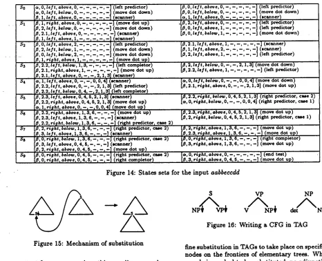
A n example

W e give one example that illustrates h o w the recognizer works. T h e g r a m m a r used for the example generates the language L =

{a"b"ecndn]n >

0}. The input string given to the recognizer

is:

aabbeccdd.

The grammar is shown in Fig-

ure 12. The states sets are shown in Figure 14. Next to each state we have printed in paren- theses the name of the processor that was applied to the state. The input is recognized since

[a, O, right, above,

0 . . . - ] is in states set

sg.

3 . 6

Remarks

U s e of m o v e dot u p a n d m o v e dot d o w n M o v e dot d o w n and m o v e dot up can be eliminated in the algorithm by merging the original dot and the position it is m o v e d to. However for explana- tory purposes we chose to use these two processors in this paper.

Off-llne vs on-line

T h e algorithm given is an off-line recognizer. It can be very easily modified to work on line by adding an end marker to all initial trees in the

grammar (see Figure 13).

Extracting a parse

The algorithm that we describe in section 3.3 is a recognizer. However, if we include pointers from a state to the other states which caused it to he

placed in the states set, the recognizer can be mod-

ified to produce all parses of the input string.

3.7 Correctness

T h e correctness of the parser has been proven and is fully reported in Schahes and Joshi (1988). It consists of the proof of the invariant given in section 3.2. O u r proof is similar in its concept to the proof of the correctness of Earley's parser given in A h o and Ullman 1973. T h e "ofily if" part of the invariant is proved by induction on the number of states that have been added so far to all states sets. T h e "if" part is'proved by induction on a defined rank of a state. T h e soundness (the algorithm rec- oguizes only valid strings) and the completeness (if a string is valid, then the algorithm will recognize it) are corollaries of this invariant.

3.8 Implementation

T h e parser has been implemented on Symbolics Lisp machines in Flavors. More details of the actual implementation can be found in Schabes mad Joshi (1988). T h e current implementation has an O(IGlZn 9) worst case time complexity and

O(IGln

6)

worst case space complexity. W e have not as yet been able to reduce the worst case time complexity to O([G[Zn6). W e are currently at- tempting to reduce this bound. However, the main purpose of constructing an Parley-type parser is to improve the average complexity, which is crucial in practice.

4

E x t e n s i o n s

W e describe h o w substitution is defined in a T A G . W e discuss the consequences of introducing substitution in T A G s . T h e n we show h o w substitution can be parsed. W e extend the parser to deal with feature structures for T A G s . Finally the relation- ship with PATR-II is discussed.

4.1 Introducing

substitution

in

T A G s

[image:8.612.65.275.75.252.2]

(9)

So

.$1

$2

$a

S4 S5 S6

$7

ss

s9

[a, O, left, above, 0 . . . - ] (left predictor)

[¢~, O, l e f t , below, O, - , - , - , - , -~ (move dot down)

[~! Zp l e f t , ahoy% 01 - - , - - r - - , - - , - - 2 (scanner)

1, right, abo~e, 0, --, - , --, --, - ] (move dot up)

2, l e f t , below, 0, --, --, --, --, - ] (move dot down) [~, 2.1, left, above, O, - , - , - , - , - ] (scanner)

z, l e / t t . b o v e , Z, , , ,

,-] ~sc~ner)

l e f t ° h a . 2 - - , - - - i ( l e f t

[/~, 2, l e f t , below, 1 . . . - ] (move dot down)

O, left, below, 2, --, --, - , --, --] (move dot down)

[~', 1, right, above, 1, - t --1--, --,--] ~move dot

up)

[0, 2.2, l e f t , below, 1, 3, --,--, --,--] ~left completor) [/~, 2.1, right, above, I, --, --, --, --, --] (move dot up)

[~, O, l e f t , above, 0, - . . . . - ] (left predictor)

f/J, O, l e f t , below, 0, - , - , - , - , - ] (move dot down)

-]

~scanner)

[ct, 11 le~t l aboo% 0 r -1 --I --P - , (left predictor)

,[~, 2, l e f t , above, O, - , - , - , - ,

[13, O, l e f t , above, 1, - , - , - , - , - ] (left predictor)

[0, O, left, below, 1, - , --, --, - , --] (move dot down)

[/~, 2.1, left, aboue, 1, --, --, - , - , - ] (scanner)

[B, 1, l e f t , above, 2, - , --, --, - , --] (scanner) [/~, 2, l e f t , above, 1, --, - , --, --, - ] (left predictor) [0, 2, l e f t , below, 0, - , - , 2, 1,3] (move dot down)

[~, 2.2, l e f t , above, 1, - , - , - , - , - ] (left predictor) [p, 2.1, le/t, abate, O, - , - , 211, a I (scanne 0

[o, 1, left, above, O, --, --, O, O, 4] (manner) [~, 2.2, f e l l abo~e, O, - , - , 2, 1, 3] (left predictor) [~, 2.2, le)'t, below, O, 4, --, 2, 1,3] (left completor) [0, 2.3, l e f t , abooe, O, 4, 5, 2 , 1 , 3 ] (scanner)

[~, 2.2, right, above, 0, 4, 5, 2, 1, 3] (move dot u p )

[a~ 1, right, above t O r --t --w 01014] (move dot up) [0, 2.2, right, above, 1, 3, 6, - , - , - ] (move dot up) [~, 2.3, l e f t , above, 1, 3, 6, --, - , - ] (scanner)

[~, 2.2, right, below, 1~ 3~ 6~ -~ - r - ] (right predictor r case 2) [0, 2, right, below, 1,3, 6 , - - , - , - - ] (right predictor, case 2)

B I 3, l e p , above, 1,3, 6, - I --I--1 (scanner)

~, O, right, below, I, 3, 6, --, --, - ] (right predictor, case 2)

[~, 3, l e f t , above, 0, 4, 5, --, --, --] (scanner) (move dot

up)

[~1 21 fish'1 oh°re10, 41 51 --, --I -- (right predictor, case 2)

[~, O, right, below, O, 4, 5, - , - ,

[~, O, rlqht l above, O, 4, 5, --, --, --] (right completor)

[a, 0, l e f t , beio~, 0, --, --, 0, 0, 4] (move dot down) [0, 2.1, right, above, 0, --, --, 2, 1,3] (move dot up)

[[3, 2.2, right, below, 0, 4, 5, 2,1,3] (right predictor, case 2) [a, 0, right, below, O, - , - , O, O, 4] (right predictor, case 1) [0, 2.8, right, above, 0, 4, 5, 2, 1, 3] (move dot up)

LS, 2, right, below, O, 4, 5, 2,1,3] (right predictor, case 1)

[0, 2, right, above, 1,3, 6, --, --, --] (move dot up)

I

B r 2.31 right I above, 113, 61 --I --~--] (move dot up)

/3, O, right, above, I, 3, 6, --, --, --] (right completor)

[0, 3, right, abo~e, 1,3, 6, --, --, --] (move dot up)

[o, O, right, above, O, --, --, --, - , - ] (end test)

[~, 3, r i g h t , above, O, 4, 5, - , --, --] (move dot up)

Figure 14: States sets for the input aabbeccdd

/\

Figure 15: Mechanism of substitution

context free grammar since this encoding uses ad- junction.

Substitution is the basic operation used in CFG. A CFG can be viewed as a tree rewriting system. It uses substitution as basic operation and it con- sists of a set of one-level trees. Substitution is a less powerful operation than adjunction.

However, recent linguistic work in TAG gram- mar development (Abeilld, 1988) showed the need for substitution in TAGs as an additional opera- tion for obtaining appropriate structural descrip- tions in certain cases such as verbs taking two sen- tential arguments (e.g. "John equates solving this problem with doing the impossible") or compound categories. It has also been shown to be useful for lexical insertion (Schabes, Abeind and Joshi, 1988). It should be emphasized that the intro- duction of substitution in TAGs does not increase their generative capacity. Neither is it a step back from the original idea o f TAGs.

D e f i n i t i o n 6 ( S u b s t i t u t i o n in T A G ) We de-

$ VP NP

Figure 16: Writing a CFG in TAG

fine substitution in TAGs to take place on specified nodes on the frontiers of elementary trees. When a node is marked to be substituted, no adjunction can take place on that node. Furthermore, sub- stitution is always mandatory. Only trees derived from initial trees rooted by a node of the s a m e la- bel can be substituted on a substitution node. The resulting tree is obtained by replacing the node by the tree derived from the initial tree. Substitution is illustrated in Figure 15.

We conventionally mark substitution nodes by a down arrow (1).

As a consequence, we can now encode directly a CFG in a TAG with substitution. The resulting TAG has only one-level initial trees and uses only substitution. An example is shown in Figure 16.

4.2

Parsing s u b s t i t u t i o n

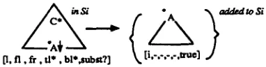
[image:9.612.44.510.76.454.2]

(10)

[I, fl, ft. fl*, bl*,subs~?] ~ . [i,-.-,-.-.W~e]

Figure 17: Substitution Predictor

T h e left predictor is restricted to apply to nodes to which adjunction can be applied.

A flag

subst? is

added to the states. When set, it indicates that the tree (initial) has been predicted for substitution. We use the index ! (as in Earley's original parser) to know where it has been predicted for substitution. When the initial tree that has been predicted for substitution has been totally recognized, we complete the state as Earley's original parser does.

A s t a t e s is now an l l - t u p l e

• [~, dot, side,poe, l, fl, fr, star, t~, b~, subst?]:

where

subst?

is a boolean that indicates whether the tree has been predicted for substitution. The other components have not been changed.

We add two more processors to the parser.

S u b s t i t u t i o n P r e d i c t o r

Suppose that there is a dot to the left of and above a non-terminal symbol on the frontier A that is marked for substitution (see Figure 17). Then the algorithm predicts for substitution all initial trees rooted by A and tries to recognize the initial tree. This operation is performed by the s u b s t i t u t i o n p r e d i c t o r .

It applies t o

s - [~,

dot, left, above, l, f l, fr , star, t~ i b~ , subst?]

such that

a(dot)

is a non-terminal on t h e

frontier of ~ .hieh is m a r k e d for

subst itut ion: It adds the states

{[fl, O, left, above, i, - , - , - , - , - , true]

]/~ i s an L n i t i a l tree s . t . # ( O ) --

or(dot)}

to

Si.

S u b s t i t u t i o n C o m p l e t o r

Suppose that the initial tree that we predicted for substitution has been recognized (see Figure 18). Then the algorithm should try to recognize the rest of the tree in which we predicted a substitution. This operation is performed by the s u b s t i - t u t i o n c o m p l e t o r .

[i'.fl',fr',tl*'.bl*',subst?']

_ .

[I.fl,fr.-.-,=uel [r,fl',fr',tl*',bl *',subst?']

Figure 18: Substitution completor

It a p p l i e s to

s = [ a , O , rioht,above, l, , , , , , t r u e ]

F o r all states s =

[/3, dot', left, a~-v~o e,- l',jt,jr,star',"

"

t~', b~', subst?']

i n Sa s . t .

#(dot')

i s marked f o r

s u b s t i t u t i o n and

l~(dot) = a(O).

I t a d d s the following stats to

Si:

[/3, dot', right, above, 1', f[ , f~, star', t~' , b~ ', subst?'] .

C o m p l e x i t y

The introduction of the substitution predictor and the substitution completor does not increase the complexity of the overall TAG parser.

I f we encode a CFG with substitution in TAG, the parser behaves in O(IGl~n s) worst case time

and O([GIn 2)

worst case space like Earley's original parser. This comes from the fact that when there are no auxiliary trees and when only substitution is used, the indices

f t , f i , t ~ , b ~

of a state will never be set. T h e algorithm will use only the substitution predictor and the substitution eom- pletor. Thus, it behaves exactly like Earley's original parser on CFGs.

4.3

P a r s i n g f e a t u r e s t r u c t u r e s for

T A G s

[image:10.612.72.263.77.125.2]

(11)

t br t U u " m

br

f t f

..- I, Ubr

Figure 19: Updating of features

A

NP V p (a)

I

/ \

PRO V PP

/ \

to go to the movies

S.top::gtsnsed> = +

S,bottom::<tensed> = V.boRom::<tensed> V.bottom::<tensed> = -

F e a t u r e s t r u c t u r e s in T A G s

As defined by Vijay-Shanker (1987) and Vijay- Shanker and 30shi(1988), to each adjunction node in an elementary tree two feature structures are attached: a top and a bottom feature structure. The top feature corresponds to a top view in the tree from the node. The b o t t o m feature corresponds to the bottom view. When the derivation is com- pleted, the top and b o t t o m features of all nodes are unified. If the top and bottom features of a node do not unify, then a tree must be adjoined at that node.

This definition can be trivially extended to substitution nodes. To each substitution node we at- tach two identical feature structures (top and bottom).

The updating of features in case of adjunction is shown in Figure 19.

U n i f i c a t i o n e q u a t i o n s

As in PATR-II, we express with unification equations dependencies between DAGs in an elementary tree. The system therefore consists of a TAG and a set of unification equations on the DAGs associated with nodes in elementary trees.

An example of the use of unification equations in TAGs is given in Figure 20. Note that the top and b o t t o m features of node S in (~ can not be unified. This forces an adjunction to be performed on S. Thus, the following sentence is not accepted:

* t o g o 1;o 1;he m o v i e s .

The auxillm-y tree 81 can be adjoined at S in or: J o h n wan1;s 1;o go 1;o 1;he m o v i e s .

But since the bottom feature of S has tensed value - in c~ and since the bottom feature of S has tensed value -4- in/32, /31 can not be adjoined at node S in a:

"Bob 1;hinks 1;o g o I;o 1;he movies.

But/~2 can be adjoined in 81, which itself can be

adjoined in a:

Bob t h i n k s John wan1;s 1;o go I;o 1;he

$

A

N P VP ([~1)

A / \

John V S 1

I

wltnu

S.top::<tensed> . +

S.bottorn::<lensed=, . V . b o l l o m : : < t e n s e d > S _ l . b o n o m : : < t e n s e d > . , V . b o t t o m : : < t e n s e d - S l > V . b o t l o m : : < t e n s e d . S l > ,. -

V.boRom::<tensed> . +

S

A

NP VP QB2)

A / \

Bob V S I

l

~ k s

S.top::<tensed> . +

S . b o t t o m : : < t e n s e d > . V . b o t l o m : : < t e n s e d > S 1 . b o t t o m : : < l e n s e d > . V . b o t t o m : : < l e n s e d - S l > V . b o n o m : : < t e n s e d - S l > . +

V . b o n o m : : < l e n s e d > ,. ÷

Figure 20: Example of unification equations

m o v i e s .

[image:11.612.84.293.60.181.2] [image:11.612.347.507.86.489.2]

(12)

P a r s i n g a n d t h e r e l a t i o n s h i p w i t h P A T r t - I I

By adding to each state the set of DAGs corresponding to the top and bottom features of each node, and by making sure that the unification equations are satisfied, we have extended the parser to parse TAGs with feature structures.

Since we introduced substitution and since we are able to encode a CFG directly, the system has the main functionalities of PATtt-II. The system parses unification formalisms that have a CFG skeleton and a TAG skeleton.

5

C o n c l u s i o n

We described an Earley-type parser for TAGs. We extended it to deal with substitution and feature structures for TAGs. By doing this, we have built a system that parses unification formalisms that have a CFG skeleton and also those that have a TAG skeleton. The system is being used for Tree Adjoining Grammar development (AbeiU~, 1988). This work has led us to a new general parsing strategy (Schabes, Abeill~ and Joshi, 1988) which allows us to construct a two-stage parser. In the first stage a subset of the elementary trees is ex- tracted and in the second stage the sentence is parsed with respect to this subset. This strategy significantly improves performance, especially as the grammar size increases.

R e f e r e n c e s

Abeill~, Anne, 1988. A Computational Grammar for

French in TAG. In Proceeding of the 12 th International

Conference on Computational Linguistics.

Aho, A. V. and Ullman, J. D., 1973. Theory of

Parsing, Translation and Compiling. Vol I: Parsing.

Prentice-Hall, Englewood Cliffs, NJ.

Earley, J., 1970. An Efficient Context-Free Parsing

Algorithm. Commun. ACM 13(2):94-102.

Joshi, Aravind K., 1985. How Much Context- Sensitivity is Necessary for Characterizing Structural Descriptions - - Tree Adjoining Grammars. In Dowry,

D.; Karttunen, L.; and Zwicky, A. (editors), Natural

Language P r o c e s s i n g - Theoretical, Computational and Psychological Perspectives. Cambridge University Press, New York. Originally presented in 1983.

2oshi, Aravind K., 1987. An Introduction to Tree Ad- joining Grammars. In Manaster-Ramer, A. (editor),

Mathematics of Language. John Benjamins, Amster- dam.

Joshi, A. K.; Levy, L. S.; and Takahashi, M., 1975.

T~ee Adjunct GraJnmars. J. Comput. Syst. Sci. 10(1).

Kroch, A. and Joshi, A. K., 1985. Linguistic Relevance

of Tree Adjoining Grammars. Technical Report MS- CIS-85-18, Department of Computer and Information Science, University of Pennsylvaain.

Schabes, Yves and Joahi, Aravind K., 1988. An

Earley.type Parser for Tree Adjoining Grammars.

Technical Report, Department of Computer and In- formation Science, University of Pennsylvania.

Schabes, Yves; Abeill~, Anne; and Joshi, Aravind K , 1988. New Parsing Strategies for Tree Adjoining

Grammars. In Proceedings of the 12 th International

Conference on Computational Linguistics.

Shieber, Stuart M., 1984. The Design of a Computer

Language for Linguistic Information. In 22 ~ Meet-

ing of the Association for Computational Linguistics,

pages 362-366.

Shieber, Stuart M., 1986. An Introduction to Unifi-

cation.Based Approaches to Grammar. Center for the Study of Language and Information, Stanford, cA.

Vijay-Shanker, K., 1987. A Study of Tree Adjoining

Grammars. PhD thesis, Department of Computer and Information Science, University of Pennsylvania.

Vijay-Shanker, K. and Joshi, A. K., 1985. Some Com- putational Properties of Tree Adjoining Grammars.

In 23 rd Meeting of the Association for Computational

Linguistics, pages 82-93.

Vijay-Shanker, K. and Joshi, A.K., 1988. Feature Structure Based Tree Adjoining Grammars. In Pro-