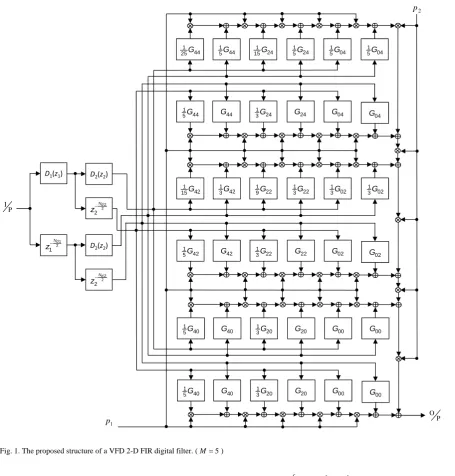
Abstract—In this paper, a new structure is proposed for the
computational design of variable fractional-delay (VFD) 2-D FIR digital filters. Based on the Taylor series expansion of the desired frequency response, a prefilter-subfilter cascaded structure can be derived. For the 1-D differentiating prefilters and the 2-D quadrantally symmetric subfilters, they can be designed simply by the least-squares method. Design example shows that the required number of independent coefficients of the proposed system is much less than that of the existing structure, while the performance of the designed VFD 2-D filters is still better under the cost of larger delays.
Index Terms— Farrow structure, variable fractional-delay filter, 2-D FIR filter, least-squares method, 2-D quadrantally symmetric filter, subfilter.
I. INTRODUCTION
onventionally, the transfer function of a variable fractional-delay (VFD) 2-D FIR digital filter is given by
(
)
1 2(
)
1 2 1 2
1 2
1 2 1 2 1, 2 1 2
0 0
, , , ,
N N
n n
n n n n
H z z p p h p p z− z−
= =
=
∑ ∑
(1)where
(
)
(
)
1 21 2
1 2
1 2 1 2 1 2 1 2
0 0
, , , , .
M M
m m
n n
m m
h p p h n n m m p p
= =
=
∑ ∑
(2) Hence, (1) can be represented by(
)
(
)
1 21 2 1 2
1 2 1 2 1 2 1 2
0 0
ˆ
, , , ,
M M
m m
m m
m m
H z z p p G z z p p
= =
=
∑ ∑
(3)where the 2-D subfilters
(
)
1 2(
)
1 2 1 2
1 2
1 2 1 2 1 2 1 2
0 0
ˆ , , , , ,
N N
n n
m m
n n
G z z h n n m m z− z −
= =
=
∑ ∑
(4)and the system can be implemented by a 2-D Farrow structure [1].
Manuscript received October 8, 2012; revised November 10, 2012. This work was supported by the National Science Council, Taiwan, under Grants NSC 101-2221-E-390-011.
Jong-Jy Shyu and Yu-Shiang Chen are with Department of Electrical Engineering, National University of Kaohsiung, Kaohsiung, Taiwan (Phone:886-7-5919236; Fax:886-7-5919374; e-mail: [email protected], [email protected]).
Soo-Chang Pei and Yun-Da Huang are with Graduate Institute of Communication Engineering, National Taiwan University, Taipei, Taiwan (e-mail:[email protected], [email protected]).
VFD digital filters belong to the branch of variable digital filters which are applied to where frequency characteristics need to be adjusted online without redesigning the system. For the past decade, several works have been proposed for the design of variable digital filters [1]-[17] due to their wide applications in signal processing and communication systems. By the function, they are generally classified into two main categories. One is the filters with variable magnitude characteristics such as cutoff frequencies or magnitude responses [2]-[8], and the other is the filters with variable fractional delay [1][9]-[17].
In this paper, the design of VFD 2-D FIR digital filters will be investigated. Comparing with the conventional 2-D Farrow structure presented recently in [1], a prefilter-subfilter cascaded structure is proposed. The structure is developed based on the Taylor series expansion of the desired frequency response. In [1], there are four types of 2-D quadrantally symmetric/ antisymmetric filters [18][19] to be designed. But, only two 1-D differentiating prefilters and one type of 2-D quadrantally symmetric subfilters are needed to be designed in this paper. By the closed relationships among the proposed structure, the required number of independent coefficients of the designed sysem is much less than that in [1] while the performance of the designed filters is still better than that in [1] under the cost of larger delays. The phenomenon will become significant for wider band VFD 2-D filter design by using higher-order 1-D prefilters and lower-order 2-D subfilters.
This paper is organized as following. In Section II, the proposed prefilter-subfilter cascaded structure is derived from the Taylor series expansion of the desired frequency response. And the design of the mentioned prefilters and subfilters for even M is presented in Section III. For simplicity, the general least-squares method is applied, and design example will be presented to demonstrate the effectiveness of the presented method. Finally, the conclusions are given in Section IV.
II. THE PROPOSED STRUCTURE
For designing a VFD 2-D FIR filter, the desired frequency response is given by
(
)
(
)
1(1 1) 2(2 2)1, 2, 1, 2 1, 2
j I p I p
d
H ω ω p p =M ω ω e− ⎡⎣ω + +ω + ⎤⎦ (5) where M
(
ω ω1, 2)
is the desired magnitude response, I1 andA New Structure and Design Method for Variable
Fractional-Delay 2-D FIR Digital Filters
Jong-Jy Shyu, Soo-Chang Pei, Yun-Da Huang and Yu-Shiang Chen
2
I are the prescribed group-delays with respect to ω1- axis and ω2- axis , respectively, and p p1, 2∈ −
[
0.5, 0.5]
. For simplicity, only quadrantally symmetric magnitude response(
1, 2)
M ω ω is considered in this paper. By Taylor series expansion,
( )
(
)
(
)
(
)
(
)
1 2
1 1 2 2
1 2
1 2
1 2
1 1 2 2
1 2
0 0
1 1 2 2
1 2
0 0
! !
! !
m m
j p p
m m
m m
M M
m m
j p j p
e
m m
j p j p
m m
ω ω ω ω
ω ω ∞ ∞ − + = = = = − − = ⋅ − − ≈ ⋅
∑
∑
∑
∑
(6)for sufficiently large M. In this paper, the case for odd M is considered first, and the case for even M will be discussed in Section IV. Let M =2Mˆ +1, then (6) becomes
( )
( ) (
( )
)
(
)
( ) (
( )
)
( ) (
(
)
)
(
)
( ) (
(
)
)
( )
(
( ) (
) (
)
)
(
)
( )
1 1 2 2
1 1 1
1
1 1
2 2 2
2 2 2 1 2 1 2 1 2 1 2
ˆ 2 ˆ 2
1 1 1 1
1 1
1 1 1
0 0
ˆ 2 ˆ 2
2 2 2 2
2 2
2 2 2
0 0
ˆ ˆ 2 2
1 1 2 2
1 2
0 0
1 1
1 1
2 ! 2 1 2 !
1 1
2 ! 2 1 2 !
1
2 ! 2 ! 1
j p p
m m m
M M
m
m m
m m m
M M m m m m m M M m m m m m m e p p j p
m m m
p p
j p
m m m
p p m m j p ω ω ω ω ω ω ω ω ω ω ω − + = = = = + = = + ⎡ − ⎤ ⎢ ⎥ ≈ − + − × + ⎢ ⎥ ⎣ ⎦ ⎡ − ⎤ ⎢ − + − ⎥ + ⎢ ⎥ ⎣ ⎦ = − − + −
∑
∑
∑
∑
∑ ∑
(
) (
)
( ) (
)
(
)
( )
(
( ) (
) (
)
)
(
)(
)
( )
(
)(
)
(
( ) (
) (
)
)
1 2 1 21 2 1 2
1 2
1 2 1 2
1 2
ˆ ˆ 2 2
1 1 2 2
1 1 2
0 0
ˆ ˆ 2 2
1 1 2 2
2 2
2 1 2
0 0
1 2 1 2
ˆ ˆ 2 2
1 1 2 2
1 2 1 2
0 0
2 1 2 ! 2 !
1
2 1 2 ! 2 !
1
(7)
2 1 2 1 2 ! 2 !
m m
M M
m m
m m m m
M M
m m
m m m m
M M
m m
p p
m m m
p p
j p
m m m
j j p p
p p
m m m m
ω ω ω ω ω ω ω ω ω = = + = = + = = + − + − + + − − × − + +
∑ ∑
∑ ∑
∑ ∑
By (5) and (7), the transfer function of the VFD 2-D FIR filter is represented by
(
)
(
)
( )
(
)
( )
(
)
( ) ( )
(
)(
)
1 22 2 1 2
1 2 1 2
2
2 1 2
1 2 1 2
1
2 1 2
1 2 1 2
1 2 1 2
ˆ ˆ
2 2
2 ,2 1 2 1 2
1 2
0 0
ˆ ˆ
2 1 2
1 1 2 ,2 1 2 1 2
2
1
0 0
ˆ ˆ
2 2 1
2 2 2 ,2 1 2 1 2
1
2
0 0
1 1 2 2
1 2 , , , , 1 , 2 1 1 , 2 1 1
2 1 2 1
Nd Nd
Nd Nd M M m m m m m m M M m m m m m m M M m m m m m m
H z z p p
z z G z z p p
z D z G z z p p
m
z D z G z z p p
m
D z D z
G m m − − = = − + = = − + = = = + + + + + × + +
∑ ∑
∑ ∑
∑ ∑
(
)
1 21 2 1 2
ˆ ˆ
2 1 2 1
2 ,2 1 2 1 2
0 0 , (8) M M m m m m m m
z z p +p +
= =
∑ ∑
and the proposed structure is shown in Fig. 1. In (8), the quadrantally symmetric subfilters
(
)
1 2
2m,2m 1, 2
G z z are
characterized by
(
)
(
)
1 21 2 1 2
1 2
2 ,2 1 2 1 2 1 2
0 0
, ,
g g
N N
n n
m m m m
n n
G z z g n n z− z −
= =
=
∑ ∑
(9)where Ng is assumed to be even while the Type III linear-phase prefilters D zi
( )
i , i=1, 2, are characterized by( )
( )
0
, : even, 1, 2.
di N
n
i i i i di
n
D z d n z− N i
=
=
∑
= (10)After mathematical management, the frequency response of (8) can be represented by
(
)
(
)
(
)
(
)
1 2
1 2
1 2
2 2 2 2
1 2
1 2 1 2
, , ,
ˆ , , ,
N N
Nd g Nd g
j j
j j
H e e p p
e e H p p
ω ω ω ω ω ω − + − + = (11) where
(
)
(
)
( )
(
)
( )
(
)
( ) ( )
(
)(
)
(
)
1 2 1 2 1 2 1 2 1 2 1 2 1 2 1 2 1 2 1 2 21 2 1 2
ˆ ˆ
2 2
2 ,2 1 2 1 2
0 0
ˆ ˆ
2 1 2
1 1 2 ,2 1 2 1 2
1
0 0
ˆ ˆ
2 2 1
2 2 2 ,2 1 2 1 2
2
0 0
1 1 2 2
ˆ
2 ,2 1 2
1 2
0
ˆ , , ,
ˆ , 1 ˆ ˆ , 2 1 1 ˆ ˆ , 2 1 ˆ ˆ 1 ˆ ,
2 1 2 1
M M m m m m m m M M m m m m m m M M m m m m m m m m m
H p p
G p p
jD G p p
m
jD G p p
m D D G m m ω ω ω ω
ω ω ω
ω ω ω
ω ω ω ω = = + = = + = = = = + + + + − × + +
∑ ∑
∑ ∑
∑ ∑
1 2 1 ˆ2 1 2 1
1 2 0 , M M m m m
p +p +
=
∑ ∑
(12a)
(
)
2 2(
)
(
) (
)
1 2 1 2
1 2
2 ,2 1 2 1 2 1 1 2 2
0 0
ˆ , ˆ , cos cos ,
Ng Ng
m m m m
n n
G ω ω g n n nω nω
= =
=
∑∑
(12b)
( )
2( )
( )
1
ˆ
ˆ sin , 1, 2,
Ndi
i i i i
n
D ω d n nω i
=
=
∑
= (12c)(
)
(
)
(
)
(
)
(
)
1 2 1 2 1 2 1 2 1 2 1 2 2 21 1 2
2 2 2
1 2
2 1 2
2 2 2
1 2 1 2
2 2 2
, , 0,
2 , , 1 , 0,
ˆ ,
2 , , 0, 1 ,
4 , , 1 , ,
g g
g g g
g g g
g g g
N N m m
N N N
m m
m m N N N
m m
N N N
m m
g n n
g n n n
g n n
g n n n
g n n n n
⎧ = = ⎪ ⎪ − ≤ ≤ = ⎪ = ⎨ ⎪ − = ≤ ≤ ⎪ ⎪ − − ≤ ≤ ⎩ (12d)
( )
(
2)
ˆ 2 Ndi , 1, 2.
i i
d n = d −n i= (12e)
Obviously, the integers I1 and I2 in (5) can be set as
2 2
g
di N
N i
III. DESIGN OF 2-DVFDFIRDIGITAL FILTERS WITH ODD M
In this paper, it will be dealt with first for the design of the prefilters D z1
( )
1 and D2( )
z2 , and then they are applied for the design of the subfilters(
)
1 2
2m,2m 1, 2
G z z . Design examples will be given to demonstrate the effectiveness of the presented method.
A. Design of the prefilters D z1
( )
1 and D2( )
z2By (7) and (8), the prefilters D z1
( )
1 and D2( )
z2 are usedas differentiators with magnitudes −ω1 and −ω2, respectively, and their specifications depend on the magnitude response
(
1, 2)
M ω ω in (5). For example, when the designed filter is an elliptically low-pass VFD filter with
(
)
2 2 1 2 2 2 1 2 2 2 1 2 2 2 1 2
1 2
1, 1,
,
0, 1,
p p
s s
M
ω ω
ω ω
ω ω
ω ω
ω ω
⎧ + ≤ ⎪
= ⎨
⎪ + ≥ ⎩
(13)
the prefilters D z1
( )
1 and D2( )
z2 are designed with passband edges ωp1 and ωp2, respectively, while their stopband edges are ωs1 and ωs2, respectively.Defining
( ) ( )
( )
2ˆ 1 , ˆ 2 , , ˆ di , T N i= ⎢⎡⎣di di di ⎤⎥⎦
d L (14a)
( )
sin( )
, sin 2( )
, , sin( )
2 , diT N i ωi = ⎢⎡⎣ ωi ωi ωi ⎤⎥⎦
s L (14b)
I P
1
p
2
p
O P
D1(z1) D2(z2)
− 2 2
2
Nd
z
− 1 2
1
Nd
z D2(z2)
− 2 2
2
Nd
z
1 44 5G 1
44 25G
1 24 5G 1
24 15G
1 04 5G 1
04 5G
44
G
1 44
5G 13G24 G24 G04 G04
1 42 3G 1
42 15G
1 22 3G 1
22 9G
1 02 3G 1
02 3G
42
G
1 42
5G 13G22 G22 G02 G02
40
G
1 40
5G 13G20 G20 G00 G00
40
G
1 40
[image:3.595.75.531.84.561.2]5G 13G20 G20 G00 G00
the magnitude responses Dˆi
( )
ωi of the prefilters can berepresented by
( )
( )
ˆ T , 1, 2
i i i i i
D ω =d s ω i= (15)
where the superscript T denotes a transpose operator. Hence, the objective error functions for designing the prefilters in least-squares sense can be defined by
( )
( )
2( )
20
ˆ ˆ
pi
si
i i i i i i i i
T T
i i i i i i
e D d D d
u
ω π
ω
ω ω ω ω ω
⎡ ⎤ ⎡ ⎤
= ⎣− − ⎦ + ⎣ ⎦ = + +
∫
∫
d
r d d Q d
(16) where 2 2 0 , 3 pi pi
i i i
u d
ω
ω ω ω
=
∫
= (17a)( )
0
2 ,
pi
i i i i d i
ω
ω ω ω =
∫
r s (17b)
( ) ( )
( ) ( )
0 , pi si T Ti i i i i d i i i i i d i
ω π
ω
ω ω ω ω ω ω
=
∫
+∫
Q s s s s (17c)
and the solutions are
1 1
2 , 1, 2.
i i i i
−
= − =
d Q r (18)
B. Design of the subfilters
(
)
1 2
2m,2m 1, 2
G z z
Similarly, by defining
( )
(
)
( )
(
)
00 00 2 2
ˆ ˆ ˆ ˆ 2 2
ˆ 0,0 , ,ˆ , , ,
ˆ 0,0 , ,ˆ , , (19a)
g g g g N N T N N MM MM g g g g ⎡ = ⎢⎣ ⎤ ⎥⎦
g L L
L
( ) ( )
( ) ( )
1 2
2 2
ˆ ˆ ˆ ˆ
2 2 2 2
1 2 1 2 2 1 2 2
1, , cos cos , ,
, , cos cos ,(19b)
c g g
g g
N N
ee
T
N N
M M M M
p p p p
ω ω ω ω ⎡ = ⎢⎣ ⎤ ⎥⎦ L L L
( ) ( )
( ) ( )
1 1 2 1 2 2
ˆ ˆ
2 2
1 1
1 2 1 2 2 1 2 2
, , cos cos , ,
, , cos cos ,(19c)
c g g
g g
N N
oe
T
N N
M M M M
M M
p p
p p p p
ω ω ω ω ⎡ = ⎢⎣ ⎤ ⎥⎦ L L L
( ) ( )
( ) ( )
2 2 2 1 2 2
ˆ ˆ
2 2
1 1
1 2 1 2 2 1 2 2
, , cos cos , ,
, , cos cos ,(19d)
c g g
g g
N N
eo
T
N N
M M M M
M M
p p
p p p p
ω ω ω ω ⎡ = ⎢⎣ ⎤ ⎥⎦ L L L
( ) ( )
( ) ( )
2 21 2 1 2 2 1 2 2
1 1
1 2 1 2 2 1 2 2
, , cos cos , ,
, , cos cos ,(19e)
c g g
g g
N N
oo
T
N N
M M M M
M M
p p p p
p p p p
ω ω ω ω ⎡ = ⎢⎣ ⎤ ⎥⎦ L L L
(
)
( )
( )
( ) ( )
1 2 1 2
1 1 2 2 1 1 2 2
ˆ , , ,
ˆ ˆ ˆ ˆ .
g cT ee g cT oe g cT eo g cT oo
H p p
jD jD D D
ω ω
ω ω ω ω
= + + −
(20) Therefore, the objective error function for designing the
subfilters
(
)
1 22m,2m 1, 2
G z z can be defined by
( )
(
)
(
)
(
)
( )(
)
(
) (
)
( ) ( )
(
) (
)
( )
( )
1 2 1 1 2 22
1 2 1 2 1 2
2
1 2 1 2 1 2
1 2 1 1 2 2
2
1 1 2 2
1 2 1 1 2 2
2
1 1 2 2
, , , , , , ˆ , , , , , cos ˆ ˆ , sin ˆ ˆ (21) g
g c g c
g c g c
r g g Qg
j j d
R
j p p R R T T ee oo R T T oe eo T T
e H p p H e e p p
M e H p p
M p p
D D
M p p
D D
u
ω ω
ω ω
ω ω
ω ω ω ω
ω ω ω ω ω ω ω ω ω ω
ω ω − + = − = − = + − + + − + − − = + +
∫
∫
∫
∫
dv dv dv dv where pR R Rω
=
∫ ∫∫ ∫∫
, (22a)1 2 1 2,
dω ωd dp dp
dv = (22b)
{
}
(
)
(
)
{
1 2 1 2 1 2}
0.5 , 0.5
, passbands and , stopbands (22c)
p
R R Rω p p
ω ω ω ω
= = − ≤ ≤ ∈ ∈ U U and
(
) (
)
(
) (
)
(
)
(
)
21 2 1 1 2 2
2
1 2 1 1 2 2
2
1 2
2
1 2 1 2
, cos , sin ,
, , (23a)
R
R
R
R
u M p p
M p p
M
M d d
ω
ω ω ω ω ω ω ω ω
ω ω
ω ω ω ω
= + + + = =
∫
∫
∫
∫∫
dv dv dv(
) (
)
( ) ( )
(
) (
) ( )
( )
1 2 1 1 2 2 1 1 2 2
1 2 1 1 2 2 1 1 2 2
ˆ ˆ
2 , cos
ˆ ˆ
2 , sin ,
(23b)
ee oo
R
oe eo
R
M p p D D
M p p D D
ω ω ω ω ω ω
ω ω ω ω ω ω
⎡ ⎤ = − + ⎣ − ⎦ ⎡ ⎤ + + ⎣ + ⎦
∫
∫
r c c
c c
dv
dv
( ) ( )
( ) ( )
( )
( )
( )
( )
1 1 2 2 1 1 2 2
1 1 2 2 1 1 2 2
ˆ ˆ ˆ ˆ
ˆ ˆ ˆ ˆ .
(23c)
T
ee oo ee oo
R
T
oe eo oe eo
R
D D D D
D D D D
ω ω ω ω
ω ω ω ω
⎡ ⎤⎡ ⎤ = ⎣ − ⎦⎣ − ⎦ ⎡ ⎤⎡ ⎤ + ⎣ + ⎦⎣ + ⎦
∫
∫
Q c c c c
c c c c
dv
dv
The least-squares solution can be obtained by differentiating (21) with respect to the coefficient vector g and setting the result to zero, which yields
1
1 −
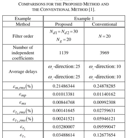
TABLE I
COMPARISONS FOR THE PROPOSED METHOD AND THE CONVENTIONAL METHOD [1].
Example Example 1
Method Proposed Conventional
Filter order 1 2 30
d d
N =N =
20 g
N = N=20
Number of independent coefficients
1139 3969
Average delays 1
-direction:
ω 25
1-direction:
ω 25
1-direction:
ω 10
1-direction:
ω 10
( )
, %
m rms
ε 0.21486344 0.24878285
mp
ε 0.01013381 0.01140162
ms
ε 0.00844768 0.00992308
( )
1,rms % τ
ε 0.00141645 0.02759631
( )
2,rms % τ
ε 0.00241521 0.05946121
1 τ
ε 0.03280007 0.09599047
2 τ
ε 0.03488614 0.12677654
C. Design examples
In this subsection, design examples are presented and the results are compared with those of the conventional method [1]. To evaluate the performance, several measured criterions are defined as below:
(
)
(
)
(
)
1 2
1
2 2
1 2 1 2 1 2
, 2
1 2 1 2
, , , , , ,
, , ,
100% , (25a)
j j
d R m rms
d R
H p p H e e p p
H p p
ω ω
ω ω ε
ω ω
⎡ − ⎤
⎢ ⎥
= ⎢ ⎥
⎢ ⎥
⎢ ⎥
⎣ ⎦
×
∫
∫
dv dv
(
)
(
)
{
(
)
}
1 2
1 2 1 2 1 2
1 2
1 2
max , , , , , , ,
passbands, 0.5 , 0.5 (25b) ,
j j
mp Hd p p H e e p p
p p
ω ω
ε ω ω
ω ω
= −
∈ − ≤ ≤
(
)
(
)
{
(
)
}
1 2
1 2 1 2 1 2
1 2
1 2
max , , , , , , ,
stopbands, 0.5 , 0.5 (25c) ,
j j
ms Hd p p H e e p p
p p
ω ω
ε ω ω
ω ω
= −
∈ − ≤ ≤
(
) (
)
1
1
2 2
1 1 2 1 2 1 1 2 1 2
, 2
1
, , , , , ,
100% , (25d)
d R rms
R
p p p p
p
τ
τ ω ω τ ω ω ε
⎡ − ⎤
⎢ ⎥
= ⎢ ⎥
⎢ ⎥
⎣ ⎦
×
∫
∫
dv dv
(
)
(
)
2
1
2 2
2 1 2 1 2 2 1 2 1 2
, 2
2
, , , , , ,
100% , (25e)
d R rms
R
p p p p
p
τ
τ ω ω τ ω ω ε
⎡ − ⎤
⎢ ⎥
= ⎢ ⎥
⎢ ⎥
⎣ ⎦
×
∫
∫
dv dv
(
)
(
)
{
(
)
}
1 1 1 2 1 2 1 1 2 1 2
1 2
1 2
,
, , , , , ,
max
passbands, 0.5 , 0.5 , (25f ) ,
d p p p p
p p
τ τ ω ω τ ω ω
ε
ω ω
−
=
∈ − ≤ ≤
(
)
(
)
{
(
)
}
2 2 1 2 1 2 2 1 2 1 2
1 2
1 2
,
, , , , , ,
max
passbands, 0.5 , 0.5 (25g) ,
d p p p p
p p
τ τ ω ω τ ω ω
ε
ω ω
−
=
∈ − ≤ ≤
where τdi
(
ω ω1, 2,p p1, 2)
and τ ω ωi(
1, 2,p p1, 2)
denote the desired and actual group delays, respectively, with respect to- direction
i
ω ,i=1, 2. Meanwhile, the numbers of independent coefficients are also taken into account for comparison, which are computed as below:
Proposed method (including scale factors):
( )
2(
)
22
2 1 ˆ 1 4 ˆ 3 ˆ
g N d
N + + M+ + M+ M (26a)
Conventional method [1]:
( )
2(
)
2( )
2 22 1 1 2
N N
c s
M M
+ + + +2
( )
N2+1 N2(
Mc+1)
Ms (26b)where
2 1 2
, for even ,
1 , for odd .
M
c s
M
c s
M M M
M M + M
⎧ = = ⎪
⎨
+ = =
⎪⎩ (27)
To compute the errors in (25), the frequencies ω1 and ω2 are uniformly sampled at step size π 100 , and the variable parameters p1 and p2 are uniformly sampled at step size 1 50 .
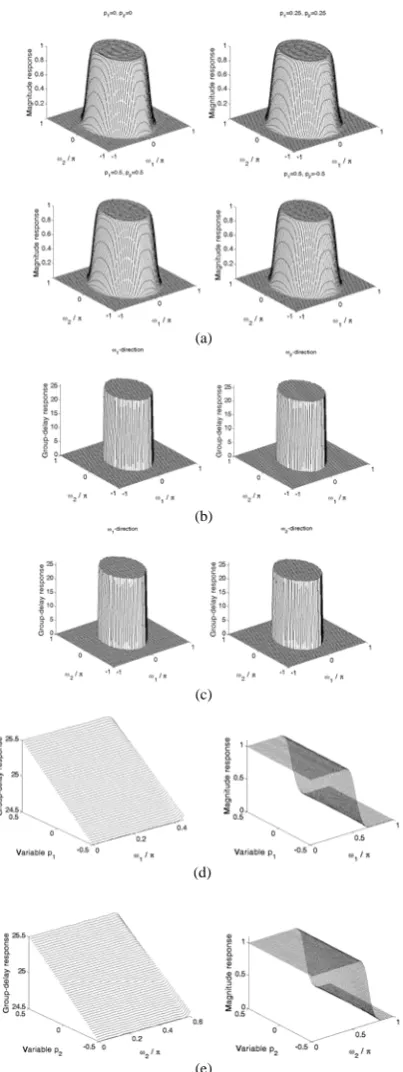
Example 1: In this example, an elliptically symmetric low-pass VFD FIR filter is designed and the desired magnitude response has been given in (13). When ωp1=0.45π , ωp2 =0.6π ,
1 0.7
s
ω = π , ωs2 =0.85π , Nd1=Nd2=30 , Ng =20 ,
5
M = , the obtained magnitude responses for
(
p p1, 2) ( )
= 0, 0 ,(
0.25, 0.25 ,)
(
0.5, 0.5 ,)
(
0.5, 0.5−)
are shown in Fig. 2(a), the group-delay responses at(
p p1, 2) (
= 0.25, 0.25)
and(
0.5, 0.5−)
are shown in Fig. 2(b) and (c), while the variable group-delay responses and magnitude responses for both2 0
ω = , p2=0 and ω1=0, p1=0 are shown in Fig. 2(d)
[image:5.595.319.532.96.330.2]and (e), respectively. The errors defined in (25) are tabulated in Table I, accompanying those of the conventional method with
20
N= .
IV. CONCLUSION
REFERENCES
[1] J.-J. Shyu, S.-C. Pei and Y.-D. Huang, “Two-dimensional Farrow structure and the design of variable fractional-delay 2-D FIR digital FIR filters,” IEEE Trans. Circuits Syst. I, Reg. Papers, vol. 56, no. 2, pp. 395-404, Feb. 2009.
[2] T.-B. Deng and T. Soma, “Design of 2-D variable digital filters with arbitrary magnitude characteristics,” Signal Processing, vol. 43, no. 1, pp. 17-27, Apr. 1995.
[3] R. Zarour and M. M. Fahmy, “A design technique for variable two-dimensional recursive digital filters,” Signal Processing, vol. 17, no. 2, pp. 175-182, June 1989.
[4] T.-B. Deng, “Design of separable-denominator variable 2-D digital filters with guaranteed stability,” Signal Processing, vol. 81, no. 1, pp. 219-225, Jan. 2001.
[5] T.-B. Deng and T. Soma, “Design of zero-phase recursive 2-D variable filters with quadrantal symmetric,” Multidimensional Systems and Signal Processing, vol.6, pp.137-158, 1995.
[6] T.-B. Deng, E. Saito and E. Okamoto, “Efficient design of SVD-based 2-D digital filters using specification symmetry and order-selecting criterion,” IEEE Trans. Circuits Syst.Ⅰ, Fundam. Theory Appl., vol. 50, no. 2, pp. 217-226, Feb. 2003.
[7] T.-B. Deng, “Design of linear-phase variable 2-D digital filters using matrix-array decomposition,” IEEE Trans. Circuits Syst.Ⅱ, Analog Digit. Signal Process., vol. 50, no. 6, pp. 267-277, Jun. 2003.
[8] J.-J. Shyu, S.-C. Pei and Y.-D. Huang, “Design of variable 2-D FIR digital filters by McClellan transformations,” IEEE Trans. Circuits Syst.
Ⅰ, Reg. Papers, vol. 56, no. 3, pp. 574-582, Mar. 2009.
[9] C. W. Farrow, “A continuously variable digital delay elements,” in Proc. 1988 IEEE Int. Symp. Circuits and Systems, vol. 3, June 1998, pp. 2641-2645.
[10] T. I. Laakso, V. Valimaki, M. Karjalainen and U. K. Laine, “Splitting the unit delay: Tools for fractional delay filter design,” IEEE Signal Processing Mag., vol. 13, pp. 30-60, Jan. 1996.
[11] T.-B. Deng and Y. Lian, “Weighted-least-squares design of variable fractional-delay FIR filters using coefficient symmetry,” IEEE Trans. Signal Process., vol. 54, no. 8, pp. 3023-3038, Aug. 2006.
[12] H. Zhao and J. Yu, “A simple and efficient design of variable fractional delay FIR filters,” IEEE Trans. Circuits Syst.Ⅱ, Exp. Briefs, vol. 53, no. 2, pp. 157-160, Feb. 2006.
[13] K. M. Tsui, S. C. Chan and H. K. Kwan, “A new method for designing causal stable IIR variable fractional-delay digital filters,”IEEE Trans. Circuits Syst.Ⅱ, Exp. Briefs, vol. 54, no. 11, pp. 999-1003, Nov. 2007. [14] T.-B. Deng, “Symmetric structures for odd-order maximally flat and
weighted-least-squares variable fractional-delay filters,“ IEEE Trans. Circuits Syst.Ⅰ,Reg. Papers, vol. 54, no. 12, pp. 2718-2732, Dec. 2007. [15] J.-J. Shyu, S.-C. Pei, C.-H. Chan, Y.-D. Huang and S.-H. Lin, “A new criterion for the design of variable fractional-delay FIR digital filters,”
IEEE Trans. Circuits Syst. I, Reg. Papers, vol. 57, no. 2, pp. 368-377, Feb. 2010.
[16] T.-B. Deng and W.-S. Lu, “Weighted least-squares method for designing variable fractional delay 2-D FIR digital filters,“ IEEE Trans. Circuits Syst.Ⅱ, Analog Digit. Signal Process., vol. 47, no. 2, pp. 114-124, Feb. 2000.
[17] C.-C. Tseng, “Design of 1-D and 2-D variable fractional delay allpass filters using weighted least- squares method,” IEEE Trans. Circuits Syst.
Ⅰ, Fundam. Theory Appl., vol. 49, no. 10, Oct. 2002.
[18] S.-C. Pei and J.-J. Shyu, “Symmetric properties of two-dimensional sequences and their applications for designing linear-phase 2-D FIR digital filters,” Signal Processing, vol. 42, no. 3, pp. 261-271, Mar. 1995. [19] R. Zhao and X. Lai, “A fast matrix iterative technique for the WLS design
of 2-D quadrantally symmetric FIR filters,” Multidimensional Systems and Signal Processing, vol.22, pp.303-317, 2011.
(a)
(b)
(c)
(d)
[image:6.595.62.264.84.621.2] [image:6.595.293.549.114.697.2]
(e)
Fig. 2. Design of an elliptically symmetric low-pass VFD FIR filter. (a) Magnitude responses at
(
p p1, 2)
=( )0, 0 , (0.25, 0.25), (0.5, 0.5),(0.5, 0.5− ). (b) ω1- directional and ω2- directional group-delay responses in the passband at