Ghazal Fazelnia
Submitted in partial fulfillment of the requirements for the degree of
Doctor of Philosophy
in the Graduate School of Arts and Sciences
COLUMBIA UNIVERSITY
Ghazal Fazelnia All Rights Reserved
Optimization for Probabilistic Machine Learning
by
Ghazal Fazelnia
We have access to great variety of datasets more than any time in the history. Everyday, more data is collected from various natural resources and digital platforms. Great advances in the area of machine learning research in the past few decades have relied strongly on availability of these datasets. However, analyzing them imposes significant challenges that are mainly due to two factors. First, the datasets have complex structures with hidden interdependencies. Second, most of the valuable datasets are high dimensional and are largely scaled. The main goal of a machine learning framework is to design a model that is a valid representative of the observations and develop a learning algorithm to make inference about unobserved or latent data based on the observations. Discovering hidden patterns and inferring latent characteristics in such datasets is one of the greatest challenges in the area of machine learning research. In this dissertation, I will investigate some of the challenges in modeling and algorithm design, and present my research results on how to overcome these obstacles.
Analyzing data generally involves two main stages. The first stage is designing a model that is flexible enough to capture complex variation and latent structures in data and is robust enough to generalize well to the unseen data. Designing an expressive and interpretable model is one of crucial objectives in this stage. The second stage involves training learning algorithm on the observed data and measuring the accuracy of model and learning algorithm. This stage usually involves an optimization problem whose objective is to tune the model to the training data and learn the model parameters. Finding global optimal or sufficiently good local optimal solution is one of the main challenges in this step.
Probabilistic models are one of the best known models for capturing data generating process and quantifying uncertainties in data using random variables and probability distributions. They are powerful models that are shown to be adaptive and robust and can scale well to large
To remedy this, they require approximate inference strategies that often results in non-convex optimization problems. The optimization part ensures that the model is the best representative of data or data generating process. The non-convexity of an optimization problem take away the general guarantee on finding a global optimal solution. It will be shown later in this dissertation that inference for a significant number of probabilistic models require solving a non-convex optimization problem.
One of the well-known methods for approximate inference in probabilistic modeling is variational inference. In the Bayesian setting, the target is to learn the true posterior distribution for model parameters given the observations and prior distributions. The main challenge involves marginalization of all the other variables in the model except for the variable of interest. This high-dimensional integral is generally computationally hard, and for many models there is no known polynomial time algorithm for calculating them exactly. Variational inference deals with finding an approximate posterior distribution for Bayesian models where finding the true posterior distribution is analytically or numerically impossible. It assumes a family of distribution for the estimation, and finds the closest member of that family to the true posterior distribution using a distance measure. For many models though, this technique requires solving a non-convex optimization problem that has no general guarantee on reaching a global optimal solution. This dissertation presents a convex relaxation technique for dealing with hardness of the optimization involved in the inference.
The proposed convex relaxation technique is based on semidefinite optimization that has a general applicability to polynomial optimization problem. I will present theoretical foundations and in-depth details of this relaxation in this work. Linear dynamical systems represent the functionality of many real-world physical systems. They can describe the dynamics of a linear time-varying observation which is controlled by a controller unit with quadratic cost function objectives. Designing distributed and decentralized controllers is the goal of many of these systems, which computationally, results in a non-convex optimization problem. In this dissertation, I will further investigate the issues arising in this area and develop a convex relaxation framework to deal with the optimization challenges.
components in the observations while too many parameters may cause significant complications in learning or overfit to the observations. Non-parametric models are suitable techniques to deal with this issue. They allow the model to learn the appropriate number of parameters to describe the data and make predictions. In this dissertation, I will present my work on designing Bayesian non-parametric models as powerful tools for learning representations of data. Moreover, I will describe the algorithm that we derived to efficiently train the model on the observations and learn the number of model parameters.
Later in this dissertation, I will present my works on designing probabilistic models in combination with deep learning methods for representing sequential data. Sequential datasets comprise a significant portion of resources in the area of machine learning research. Designing models to capture dependencies in sequential datasets are of great interest and have a wide variety of applications in engineering, medicine and statistics. Recent advances in deep learning research has shown exceptional promises in this area. However, they lack interpretability in their general form. To remedy this, I will present my work on mixing probabilistic models with neural network models that results in better performance and expressiveness of the results.
List of Figures iii
List of Tables vii
Chapter 1: Introduction 1
Chapter 2: Probabilistic Orthogonal Matching Pursuit 4
2.1 Introduction . . . 4
2.2 Probabilistic Orthogonal Matching Pursuit . . . 6
2.3 BNP dictionary learning . . . 11
2.4 Experiments . . . 15
2.5 Conclusion . . . 19
Chapter 3: Beta Process Subspace Analysis 22 3.1 Introduction . . . 22
3.2 Beta Process Subspace Analysis . . . 24
3.3 Example: Tiny Images . . . 25
3.4 Inference for BPSA . . . 27
3.5 Experiments . . . 34
3.6 Conclusion . . . 39
Chapter 4: Mixed Membership Recurrent Neural Networks 40 4.1 Introduction . . . 40
4.2 Background . . . 42
4.3 Mixed Membership RNN Models . . . 44
4.4 Experiments . . . 48
4.5 Conclusion . . . 54
5.2 Background . . . 58
5.3 Convex Relaxation for Variational Inference . . . 63
5.4 Experimental Results . . . 70
5.5 Discussion . . . 74
5.6 Conclusion . . . 74
Chapter 6: Convex Relaxation for Distributed Control Problem 76 6.1 Introduction . . . 77
6.2 Preliminaries . . . 81
6.3 Finite-horizon Deterministic ODC Problem . . . 88
6.4 Infinite-horizon Deterministic ODC Problem . . . 101
6.5 Infinite-Horizon Stochastic ODC Problem . . . 110
6.6 Extension to Dynamic Controllers . . . 117
6.7 Numerical Examples . . . 118
6.8 Conclusions . . . 124
Chapter 7: Conclusion 125
Bibliography 128
Figure 2.1 Denoising images: House, Lena, Barbara, Boat. . . 16 Figure 2.2 (Blue: K-SVD, Red: BPFA) Average SSIM results for different images and
noise settings as a function of number of dictionary elements for K-SVD, each repeated for 20 trials. The red line indicates the results for BPFA which is not a function of the x-axis. The dashed red lines are the number of dictionary elements in BPFA responsible for representing 95%, 97% and 99% of all input data. . . 17 Figure 2.3 Two masks considered. Left: 1D Cartesian sampling with random phase
encodes (30% sample rate shown); Right: 2D random sampling (25% sample rate shown). . . 18 Figure 2.4 (left) Original Shoulder, (middle) Shoulder distorted by Cartesian 35%
mask, (right) Shoulder distorted by Cartesian 35% mask and noise withσ = 0.05. 19 Figure 2.5 PSNR results in the noiseless setting for different MRI, masks and sampling
percentages. PrOMP for EM outperforms MCMC for the same BNP dictionary learning model. . . 20 Figure 2.6 PSNR results with additive sampling noise (σ = 0.05) for the lumbar
MRI, using the Cartesian (left) and Random (right) masks and different sampling percentages. PrOMP outperforms MCMC for the same BNP dictionary learning model. . . 21 Figure 2.7 Stem plots ofπk (sorted) for lumbar MRI with Cartesian 25% sampling
mask. PrOMP (bottom) shows the expectation and MCMC (top) shows the best performing iteration. PrOMP learns a much sparser representation for this model. 21
image. From left to right, subspaces are ordered to show the most used to the least used ones in image representation. . . 26 Figure 3.2 Probabilities of using each dictionary subspace in representing images
ordered form the most probable to the least. . . 27 Figure 3.3 A histogram of number of subspaces used in representing 100,000 randomly
selected images. . . 28 Figure 3.4 Accuracy of the Bessel approximation in Eq. (3.14) and (3.15) (with
δ= 1, D= 25,d= 100). (left) The true and approximate functions, (middle) the absolute error of the approximation, (right) the approximation error as a fraction of the true value. . . 33 Figure 3.5 Images used in our denoising experiments: House, Peppers, Lena, Barbara. 36 Figure 3.6 A histogram of the subspace dimensionality for σ = 15. Many inferred
subspaces are one dimensional, similar to BPFA and K-SVD, but BPSA learns subspaces with other sizes as well. . . 38 Figure 3.7 The average number of vectors used from the dictionary by a patch for
various noise settings. For BPSA, since all vectors in an activated subspace are used, we calculated this number by summing the dimensionality of each subspace used by a patch. . . 38 Figure 3.8 The 13 most probable subspaces learned from the “House” image with
σ= 15. . . 39 Figure 4.1 The unrolled proposed framework we use in our experiments shown for
thedth sequence. Each prediction uses a weighted combination of an RNN and a customer-specific parameter. As the time between observations decreases the RNN prediction is favored more heavily. As the time lag increases the prediction is more biased towards an independent distribution parameterized by φd. (This
difference is indicated by arrow thickness above.) . . . 42 Figure 4.2 MM-RNN graphical model. . . 47
0
reduces to its base LSTM model. An increase in κ indicates that this RNN prediction is being forgotten more quickly as the time between orders increases and the customer-level base distribution is being used instead. As is evident, a combination of sequential/non-sequential modeling gives more accurate predictions. (b) The error between the aisle distribution and predicted distribution for the
last order as a function of time passed since the previous order. We use our basic MM-RNN model (with κ= 0.1) and compare with an LSTM RNN (equivalent to κ= 0). As is evident, the LSTM decreases in predictive performance as more time passes between observations. Whenρ≡0, the model reduces to an exchangeable model on orders, giving further support to our belief in the decreasing sequential value as time lag increases. . . 50 Figure 4.4 (a) Boxplot of MSE using the aisle level data when t0 = 1 for Instacart.
Similar to the product level case, a combination of sequential/nonsequential modeling gives more accurate predictions. (b) Exploratory results on UK retail dataset. Prediction error for the last order of the users as a function of days since their prior purchase. The details of what is being shown is the same as Figure 4.3(b) (please see caption for description), only cross entropy was used here, and the time lag is not truncated at 30 days in the dataset. The wider error bars are due to the fewer customers and greater variation in time lag. . . 52 Figure 5.1 Constructed graph for the optimization problem (5.9) on the left side,
and its tree decomposition on the right side. Some edges are removed for better legibility of the graphs. . . 65
improvement of CRVI over CAVI for 100 simulations using different prior hyper-parameters and initializations. After calculating the respective local optimal variational objective functions, the value found by CAVI is subtracted from the value from CRVI and divided by the values from CAVI to obtain the relative improvement score. As is evident, CRVI gave a significant improvement over CAVI. 72 Figure 5.3 The fraction of agreement in the recoveredZ’s with original Z using CRVI
and K-SVD (here, OMP). The x-axis shows the probability of a 1 in every entry
of the original sparse matrix. . . 73
Figure 5.4 The fraction of correctly recovered 1’s in the original Z using CRVI and K-SVD (here, OMP). The x-axis shows the probability of a 1 in every entry of original sparse matrix. . . 74
Figure 6.1 A minimal tree decomposition for a ladder graph. . . 83
Figure 6.2 picture2 . . . 89
Figure 6.3 picture10 . . . 93
Figure 6.4 The sparsity graph for the infinite-horizon deterministic ODC in the case where K consists of diagonal matrices (the central vertex corresponding to the constant 1 is removed for simplicity). . . 107
Figure 6.5 The ratio λ2 λ1 obtained from the dense SDP relaxation of the finite-horizon ODC Problem (6.26) for 100 random systems. . . 119
Figure 6.6 Optimal degrees of different relaxations for 100 random systems. . . 120
Figure 6.7 picture5 . . . 121
Figure 6.8 Two different structures (decentralized and distributed) for the controller K: the free parameters are colored in red (uncolored entries are set to zero). . . . 122
Figure 6.9 picture6 . . . 122
Figure 6.10 The optimality degree and optimal cost of the near-optimal controller designed for the mass-spring system for two different control structures. The noise covariance matrix Σv is assumed to be equal to σIr, whereσ varies over a wide range. . . 123
Table 2.1 SSIM |PSNR performance. K-SVD sees the ground truth when choosing the number of dictionary elements for each image. . . 14 Table 3.1 SSIM |PSNR for image as a function of noise standard deviation. . . 37 Table 4.1 Quantitative evaluation comparing with other approaches using mean
squared error (MSE) and cross entorpy loss (CEL). Direct imputation approaches perform the worst. LSTM-based approaches tend to outperform GRU-based approaches, while our time-adaptive approach tends to improve performance of these respective architectures. Thus, the proposed MM-RNN approach is able to use time between observations to improve predictive performance. . . 53 Table 5.1 Information about the datasets, running time of the algorithms, and rank of
the found solution using CRVI. We see that CRVI is slower than CAVI (coordinate ascent). However, the rank of the found CRVI solution is near 1 (and less than the theoretical upper bound of 3), indicating a solution nearer the global optimum. This is confirmed in Figure 5.2. . . 71
First and foremost, I would like to thank my Ph.D. advisor, Professor John Paisley. I have been extremely lucky and fortunate to have him as my academic advisor in the past few years. He inspired me with his unique vision, encouraged me with his genuine support, and enlighten me with his wisdom and knowledge. I would like to extend my thanks to Professor John Wright, Professor David Blei, Professor Javad Ghaderi, and Professor Daniel Hsu for being part of my thesis committee and providing invaluable advice. Moreover, I have had the greatest opportunity to be a part of Columbia community that have nurtured me and have become my second home. Ph.D. years have been the toughest years of my life, and none of it could have happened without support and love from my friends and family. I would like to express my deepest gratitudes to my parents, Zhila Mahdian and Saeed Fazelnia. They have given me confidence to believe in my capabilities, guidance to pursue my dreams, and support to wholeheartedly believe that women can achieve anything that men can. They have sacrificed greatly for creating better lives for our family, and I will be forever grateful for that. I would like to thank my siblings, Mohamad and Dorsa, and my uncle Behzad, for always loving me, supporting me, taking care of me, and encouraging me to go distance. Last but absolutely not least, I would like to offer my sincerest thanks to my husband, Saleh. He has been a true loving and supporting partner that anyone could ever wish for. I have been extremely fortunate for having him by my side to believe in me through my failures and disappointments, to give me courage to always do the right thing, and to truly empower me to succeed. His encouragement and vision have been great companions in my Ph.D.. I truly love him, and will always be thankful for his unconditional kindness and immerse support.
and to the love of my life Saleh.
Chapter 1
Introduction
Probabilistic models are one of the most powerful techniques for discovering and describing underlying structures in a dataset [48]. They can infer possible models to explain observed data. This approach is flexible to adjust to different variations in data and is robust to tolerate noise in data. Uncertainty in data is a crucial part for this type of models. Due to their probabilistic nature, they are capable of modeling uncertainty and incorporating it for predicting. Generative models assume a generating process from which the data is drawn. Using them enables us to not only train the model and make prediction on unobserved data but also to quantify our uncertainty about the model assumptions and prediction results. Latent variable models are a subcategory of probabilistic models which assume that data is affected by unobserved factors or latent variables. Latent variables could represent the unobserved structures in the data. Latent variable models include factor analysis models, mixture models, and latent class models among others.
Factor analysis models assume that data can be described via a linear combination of unobservable latent variables called factors. Collection of these factors is called dictionary. Sparse coding seeks to decompose data points into combination of a small subset of patterns selected from the dictionary. The goal of dictionary learning is to simultaneously learn these patterns in the dictionary (factors) and the sparse representation of the signals [2]. In this dissertation, I will present my work on dictionary learning and sparse signal representation with Bayesian nonparametric priors in which the number of factors is learned by the model [41].
I derive probabilistic orthogonal matching pursuit (PrOMP), a stochastic Expectation Maxi-mization (EM) algorithm for learning sparse data representations, and extend the algorithm to the sparse Bayesian nonparametric dictionary learning task using the beta process. The core EM algorithm provides a new way for doing inference in nonparametric dictionary learning models. Our theoretical analysis builds upon the previous theory for Orthogonal Matching Pursuit (OMP) [31, 102, 128]. Like OMP, PrOMP is a greedy algorithm for regression that iteratively selects columns of a matrix according to a score. This score is based on an atypical use of the EM algorithm and thus optimizes a marginal probability distribution [42].
Mixed membership models provide a probabilistic approach to modeling groups of data through a combination of shared and group-specific parameters [3]. A learning algorithm aims to learn the shared components alongside membership assignment weights for representing each data point using the components. In this dissertation, I will present my work on using mixed membership models when learning sequential data. Deep Neural Networks (DNN) have been widely used for modeling sequential data and have shown great performance in capturing recurring patterns in data. Models of sequential data such as the recurrent neural network (RNN) often implicitly treat a sequence as having a fixed time interval between observations and do not account for group-level effects when multiple sequences are observed. I propose a model for grouped sequential data based on the RNN that accounts for varying time intervals between observations in a sequence by learning a group-level parameter to which each sequence reverts as more time passes between observations. Our approach is motivated by the mixed membership framework, and can be used for dynamic topic modeling-type problems in which the distribution on topics (not the topics themselves) are evolving in time [45].
Probabilistic models with Bayesian hierarchical priors are powerful techniques for creating interpretable and expressive models. However, a major challenge in Bayesian modeling is posterior inference. For many models this requires calculating normalizing integrals that neither have a closed form, nor are solvable numerically in polynomial time. There are two fundamental approaches to addressing the posterior inference problem. One uses Markov chain Monte Carlo (MCMC) sampling techniques that are asymptotically exact. However, these methods tend to be slow compared with point-estimates and not scalable to large datasets [46, 58]. Mean-field
variational inference is another approach that approximates the posterior distribution by first defining a simpler family of distributions and then finding a member that is closest to the desired posterior [67] according to the KullbackLeibler (KL) divergence. This turns the inference problem into an optimization problem. This approach introduces new challenges since it mostly results in non-convex optimization problems. In this dissertation, I will present a method to deal with the non-convexities in variational inference (VI) optimization for conjugate prior models that can achieve near globally optimal solutions [43].
The proposed optimization technique is based on convex relaxation and semidefinite program-ming (SDP). In our approach, an SDP relaxation converts a non-convex polynomial optimization of vector parameters to a convex optimization with matrix parameters via a lifting technique. The exactness of the relaxation can then be interpreted as the existence of a low-rank solution to this SDP. In the last part of this dissertation, I will present theoretical details on this method as well as its implications in linear dynamical systems with decentralized controls [39].
The rest of this dissertation is organized as follows. Chapter 2 presents our results for developing inference algorithm in nonparametric Bayesian modeling. It will be followed by Chapter 3 in which I demonstrate our work on Bayesian nonparametric factor analysis model for dictionary learning and sparse representation. In chapter 4 I introduce our work on probabilistic analysis for sequential data modeling using deep learning techniques. Chapter 5 presents my work on convex relaxation process for variational inference which is followed by Chapter 6 that gives more detail about the relaxation technique and its application for linear time varying datasets. I will conclude this dissertation in the Chapter 7 and bring a discussion for the future directions.
Chapter 2
Probabilistic Orthogonal Matching
Pursuit
In this chapter, I presentprobabilistic orthogonal matching pursuit (PrOMP) for learning sparse data representations, and extend the algorithm to the sparse Bayesian nonparametric dictionary learning task using the beta process [42]. Like OMP, PrOMP is a greedy algorithm for regression that iteratively selects columns of a matrix according to a score. This score is based on an atypical use of the EM algorithm and thus optimizes a marginal probability distribution. Our theoretical analysis builds on the previous theory for OMP. We also present experimental results on dictionary learning for the image denoising and compressed sensing magnetic resonance imaging (CS-MRI) problems, where we empirically demonstrate that PrOMP, when used in a dictionary learning algorithm, can lead to improved performance over other sparse dictionary learning and inference approaches by converging to a better local optimal solution. I will expand the applications of PrOMP to more Bayesian nonparametric models in the next chapter.
2.1
Introduction
Sparse data representation is a fundamental problem of signal processing that aims to decompose data into combinations of small subsets of patterns selected from a larger dictionary. Due
to its significant applications in areas such as applied mathematics, statistics, and electrical engineering, this field has received much attention. Various methods for sparse data representation and recovery have been proposed using sparse penalties. For instance, least squares with l1
norm penalties (lasso) [23, 35, 124] are very effective in recovering sparse representation. Many fundamental approaches are build on thisl1 approach [57].
Another important family are matching pursuit (MP) methods, based on iterative greedy algorithms that search for a sparse representation of data [88]. The main idea of MP is to iteratively select columns to incorporate in the representation from a set of given patterns based on correlation with the current residual, after which the residual is updated. This greedy algorithm continues to run until reaching some convergence threshold. For example, orthogonal matching pursuit (OMP) expedites convergence to the final solution by finding the least squares solution on a growing subset of basis functions [102, 128].
The computational simplicity of OMP in addition to its effectiveness for approximating l0
minimization problems have made it a very appealing method for sparse data representation, and inspired many modifications. For example, stagewise orthogonal matching pursuit (StOMP) [31], allows for multiple simultaneous patterns to be included at once. Issues with threshold selection have been addressed in regularized OMP [92] and compressive sampling OMP [91] that are more robust to noisy conditions and are more efficient in resource usage.
In this chapter, I propose probabilistic orthogonal matching pursuit (PrOMP), which builds upon OMP via a probabilistic model. PrOMP follows an identical algorithmic outline as OMP, but with modified scores calculation and weight (posterior) updates to account for the probabilistic approach. We rigorously derive PrOMP using the expectation-maximization (EM) algorithm, meaning our objective is a marginal likelihood on the sparsity pattern. Our approach to EM, while correct, is not typical since the hidden variables used are growing based on the current active set and thus each E-M step does not correspond to the same breakdown of the marginal. We provide a theoretical analysis of PrOMP inspired by [128] for OMP, with the necessary modification.
I then extend this basic model to the dictionary learning problem using a Bayesian non-parametric beta process prior. In this problem, the additional goals are to learn the patterns
themselves based on multiple signals, as well as the number of patterns to use [70, 71, 95]. This approach has proven effective in tasks such as image denoising, inpainting [140], and compressed sensing [64]. Inference for the beta-Bernoulli process has focused on variational methods [95] and Markov Chain Monte Carlo (MCMC) sampling [64, 140] without considering scalability. We address this issue by proposing a novel scalable EM-based algorithm. [2] deals with large data sets by incorporating OMP step used by KSVD, however, our scalable extension is an EM special case of stochastic variational inference [61].
In Section 2.2 I present the problem setup and PrOMP algorithm along with detailed theoretical analysis, making connections to OMP along the way. PrOMP is extended to the sparse dictionary learning problem in Section 2.3 We present the experiments on dictionary learning in Section 5.4.
2.2
Probabilistic Orthogonal Matching Pursuit
I focus on PrOMP for sparse coding of one signal and extend to multiple observations when discussing dictionary learning in Section 2.3. Given a signalx∈Rd and matrixW∈
Rd×K, our goal is to find a sparse representations forx such thatx≈Ws. We do this via the model
x∼ N(Ws, σ2I). (2.1)
Further, we formulate s=zc wherez is a sparse binary coding that indicates the columns of W used in the representation, and c represents corresponding real-valued weights. Their respective probability distributions are
zk∼Bern(πk), c∼ N(0, λ−1I), (2.2)
thusz∈ {0,1}K andc∈
RK. The Bernoulli prior regularization will be a more significant factor for dictionary learning, where eachπk will have a beta prior.
2.2.1 PrOMP via the EM algorithm
In inference procedure, we learn a point estimate for the binary z, and conditional posterior q distribution on c. Following the general regression setup, we assume W is known here and
make the appropriate modifications for dictionary learning. In the EM algorithm, the goal is to maximize p(x,z) over the sparse coding vectorsz withc treated as the marginalized variables. To this end, we can introduce an arbitrary distribution q on these hidden variables and set up the EM objective function on the log marginal distribution,
lnp(x,z) =Eq h lnp(x,z,c) q(c) i | {z } L(z) + Eq h ln q(c) p(c|x,z) i | {z } KL(qkp) . (2.3)
We note that the sparse coding step based on Eq. (2.3) is not as straightforward as it might appear, since ifzk= 0, then the corresponding updated q distribution on ck will revert to the
zero-mean prior, which makes it effectively impossible to setzk in the following iteration. This is
a common problem encountered by Bayesian nonparametric dictionary learning algorithms [115]. However, our less conventional route will be to construct a sequence of the RHS each equal to the LHS. Define the index set A ⊂ {1, ..., K} and let cA denote the subvector ofc defined by
A. Then equivalently, lnp(x,z) =Eq h lnp(x,z,cA) q(cA) i | {z } LA(z) +Eq h ln q(cA) p(cA|x,z) i | {z } KL(qkpA) . (2.4)
We note that the RHS of Eq. (2.3) & (2.4) are equal, yet L 6= LA and KL(qkp) 6= KL(qkpA)
because they correspond to different joint distributions.1 Our key observation is that, by setting q=pA and updating z according toLA in one iteration of EM, we are monotonically increasing
lnp(x,z) regardless of the index set used for that particular iteration. This simply follows from the original proof of EM. We will see here that definingA and updatingLA in a particular way
will lead to an OMP-like algorithm.
For example, letA correspond to dimensions inz set to 1. What the equality in Eq. (2.4) shows is that we can arbitrarily integrate out portions of the vectorc corresponding to those dimensions in which zk = 0 (among other possible options). Furthermore, the conditional
posteriorp(cA|x,z) is easily shown to be Gaussian and the calculation ofLA is straightforward.
We use this observation to derive a two step greedy algorithm for jointly learning z andq(c). 1
Our two step greedy procedure first calculates the E-step in Eq. (2.4) using the current A. It then picks the dimension ofzto set to 1 that increases LA the most. Calling this dimension j, it
finally incrementsA ← A ∪ {j}. The next iteration then recomputes LA based on the augmented
set A. Therefore, each iteration optimizes over a different function LA using a q(cA) that is
growing in dimensionality. If including no dimension ofz can increaseLA, then the algorithm
terminates. Unlike OMP, for which this never can happen and thus termination criteria are necessary, the prior regularization of our Bayesian model allows for automatic termination based on the marginal likelihood.
2.2.2 The PrOMP algorithm
As discussed previously, regardless of the index setA, by settingq(cA) =p(cA|x,z) and updating
zsuch thatLA(z) increases, we are guaranteed to monotonically improve lnp(x,z). Our proposal
is to greedily add columns of W by setting the corresponding dimensions of z to 1 based on how muchLA improves. The score for dimension j is denoted byξj+−ξj−. This is the difference
between LA forzj = 1 (+) or 0 (-). For allj,ξj− will be the same for the current iteration, but
is included as a stopping criterion since it indicates whether there are noj that increasesLA, at
which point the algorithm terminates. The PrOMP outline is shown in Algorithm 1 with the equations below.
For the E-step, we have a Gaussian conditional posterior on the subset of c given by the active dimensions inz,q(cA) =N(cA|µA,ΣA) where
ΣA= (λI+W>AWA/σ2)−1, µA = ΣAW>Ax/σ2. (2.5)
Here we letWA denote the submatrix ofW formed by selecting the columns ofW indexed by
A. For a particular iteration, the likelihood p(x|z,cA) with hidden data cA is also Gaussian
where the appropriate dimensions in c have been integrated out of the joint likelihood term. Since those dimension correspond tozj = 0 (as defined by the setA), the result gives
p(x|cA,zj = 1) = N(x|WAcA, σ2I+λ−1wjw>j ),
Algorithm 1 PrOMP
1: input: Wand values (later, distributions) for each πk
2: output: Coding setAand weight distribution q(cA)
3: SetA=∅
4: For eachj, set ξj±= lnp(x,zj ={0,1}) (Eq. 2.7)
5: whilemaxj ξ+j −ξj− > 0 do
6: Setj0 = arg maxj ξj+−ξj− 7: SetA ← A ∪ {j0},zj0 = 1 and ξ+
j0 =−∞
8: Setq(cA) =p(cA|x,z) (Eq. 2.5)
9: For eachj /∈ A, update (Eq. 2.7)
ξ+j = Eq[lnp(x|cA,zj = 1)] + lnπj,
ξ−j = Eq[lnp(x|cA,zj = 0)] + ln(1−πj)
10: end while
Thus, for a given active setA, the score for activating a particular dimensionj ofz can be found. Define the approximation residual to berA=x−WAµA. Then
ξj+−ξj− = Eq lnp(x,zj = 1|cA) p(x,zj = 0|cA) (2.7) = 1 2σ2 (r>Awj)2+w>j WAΣAWA>wj λσ2+w> j wj −ln(1 +w > j wj λσ2 ) + ln πj 1−πj .
The difference between PrOMP and OMP consists of the following modification: If µA ≡
(W>AWA)−1W>Ax and ξj+−ξ
−
j ≡ (r
>
Awj)2/(wj>wj), then the OMP algorithm results. The
additional values are probabilistic terms accounting for uncertainty incA, as well as the penalty
termπj for dimension j. As mentioned above, in our extension to dictionary learning we will see
2.2.3 Theoretical guarantees for PrOMP
As seen, PrOMP consists of a modification to OMP that accounts for probabilistic uncertainty. Like the extensive theory developed for OMP, we modify these results for PrOMP by considering two general problems: (1) The sparsest representation problem, whose goal is to identify the representation of the input signal that uses the least number of atoms; (2) m-sparse problem in which the signal x is required to have anm-term representation and the goal is to identify m terms in the dictionary to representx.
Theorem 2.1 (Sparsest Representation). Assume that the sparsest representation is unique. Then, PrOMP will find that representation if
max
j /∈Aopt
dkW+A
optwjk2<1, (2.8)
and provided that ln πj
1−πj ≥ln
πj0
1−π0j and kwjk2≤ kwj0k2 for all j and j
0 in the optimal set and
outside the optimal set, respectively.
We note that the condition in Eq. 2.8 has resemblance to the Exact Recovery Condition (ERC) in [128].
Proof 2.1. Let us define WA
opt ,Wj /∈Aopt. According to Algorithm 1, at step k, in order to
select an index, we need to find aj for whichξj+−ξ−j is positive and has the highest value among all of the candidates. Suppose that we have performedk steps of PrOMP and achievedAk. Define
ρ(rAk),
maxj0∈A
opt(ξ + j0 −ξj−0)
maxj∈Aopt(ξ + j −ξ − j ) = (2.9) maxj0∈A optw > j0(rAkr > Ak+WAkΣAkW > Ak) >w j0+f(j0)
maxj∈Aoptw
> j (rAkr > Ak+WAkΣAkW > Ak) >w j+f(j) .
Note that maxj∈Aopt(ξ + j −ξ
−
j ) = maxj∈Aopt\Ak(ξ
+ j −ξ − j ) as we set ξ + j = −∞ if j have been
previously chosen and the search is only over positive score values inside or outside the optimal set. Also, the conditions of this theorem guarantee thatf(j0)< f(j). PrOMP will pick an index from the optimal set at the next step if and only ifρ(rAk)<1. PrOMP will not pick the same
index twice, and j and j0 are not previously chosen. So, in order to have ρ(rAk)<1, it suffices to have maxj0∈A optw > j0(rAkr > Ak+WAkΣAkW > Ak) >w j0
maxj∈Aoptw
> j (rAkr > Ak+WAkΣAkW > Ak) >w j <1. (2.10) Let us definerAkr > Ak+WAkΣAkW > Ak =l >
klk. Note that this decomposition is possible due to the
positive definiteness of the left hand side. The left hand side of Eq. 2.10 equals the following:
klkWAoptk2,∞ klkWAoptk2,∞ = klkWAoptW + AoptWAoptk2,∞ klkWAoptk2,∞ ≤ dklkWAoptk2,∞kW + AoptWAoptk2,∞ klkWAoptk2,∞ =dkW+A optWAoptk2,∞ = max j /∈Aopt dkW+A optwjk2 (2.11)
where k · k2,∞ is the maximum of the column-wise L2 norm for a matrix. Hence, if
maxj /∈AoptdkW +
Aoptwjk2 <1, this guarantees that PrOMP will pick an index from the optimal
set.
Theorem 2.2. [128] Let m indicate the number of columns inWAopt. Then, condition in
Theorem 2.1 holds if
dω1(m−1) +dω1(m)<1. (2.12)
In other words, this condition will recover every signal with m-term representation.
where ω1(m) represents the cumulative coherence function defined as
ω1(m) , maxΛmaxj∈Ω\ΛkW>ΛWjk1 with Λ being an index set of m columns of W, and Ω
showing all the indices . ω1(0) is set to 0. We should point out that the proof of 2.2 follows the
same steps as the ones in [128] noting that L2 norm of a vector is upper bounded by its L1 norm value.
2.3
BNP dictionary learning
In this section, we expand the sparse representation problem to learning the matrix W and probabilitiesπk using Bayesian nonparametrics (BNP) similar to previous approaches, with the
contribution being the novel inference algorithm. Extending the problem toN signals, BNP dictionary learning uses the generative process
xn∼ N(W(zncn), σ2I),
cn∼ N(0, λ−1I), zn,k∼Bern(πk),
wk∼ N(0, η−1I), πk∼beta(αKγ, α(1−Kγ)),
(2.13)
for α, γ > 0 and k = 1, . . . , K in the limit K → ∞.When K is finite but large for practical implementation, this model gives a good approximation in that it will learn a subset of indexesk such thatπk is substantial.
2.3.1 Inference for BNP dictionary learning
In the inference process, we learn point estimates forW and each z={zn}. We propose a new MAP-EM algorithm that uses PrOMP to learn sparse codings ofx={xn} withπ andc={cn}
the hidden variables. Similar to the discussion in Section 2.2, the EM algorithm now aims to maximizep(x,z,W) over z and W using the equality
lnp(x,z,W) = Eq h lnp(x,z,W,c, π) q(c, π) i | {z } L(z,W) + Eq h ln q(c, π) p(c, π|x,z,W) i | {z } KL(qkp) (2.14)
We give an outline in Algorithm 2 and the relevant new equations below. We note that PrOMP requires the modification that lnπj is replaced withEq[lnπj], and similarly for ln(1−πj), since
πj is being marginalized with EM. We discuss these values below.
First we observe that c and π are conditionally independent givenW. Furthermore, thecn
and πk are also conditionally independent in their posterior. Thus we have
q(c, π) = h QN n=1q(cn) i h QK k=1q(πk) i . (2.15)
Since this follows the factorization of p(c, π|x,z,W) we are not doing mean field variational inference.
Algorithm 2 Sparse Dictionary Learning with PrOMP 1: Initialize dictionaryW.
2: whilenot convergeddo
3: Update eachznand q(cn) (Algorithm 1∗)
4: UpdateW andq(π) with EM (Eqs. 2.16 & 2.17) 5: end while ∗Replace ln πj 1−πj withEq ln πj 1−πj
. See Sec. 2.3.1 for discussion.
After performing PrOMP to update each zn andq(cn), we update the global variablesW
and π using a straightforward application of EM as follows: E-Step: For eachk, updateq(πk) = beta(ak, bk), where
ak= αγK + N P n=1 zn,k, bk=α(1−Kγ) + N P n=1 (1−zn,k) (2.16)
and using q(cn) from PrOMP, calculate L(z,W). We note that for PrOMP we now use
Eq πk
1−πk
=ψ(ak)−ψ(bk), whereψ(·) is the digamma function.
M-Step: Letbzn= diag(zn). arg maxWL(z,W) gives
W =h N X n=1 xnµ>nbzn ih ησ2I+ N X n=1 b zn(µnµ>n + Σn)bzn i−1 . (2.17)
After updatingW and eachq(πk), we return to the PrOMP algorithm to sparse code eachxn by
updatingzn andq(cn).
Next, we present some theoretical results when learning dictionary W. We note that this optimizes the function
L(z,W) =− 1 2σ2 N X n=1 kxn−W(znµn)k2 − 1 2σ2 N X n=1 trace(Σn(W>Wznz>n)) −η 2trace(WW >) + const. (2.18)
Lemma 2.1. [108] For a general real-valued matrix M, minimizing trace(M M>) have impact on reducing the rank of M and penalizes its largest singular value.
Proposition 2.1. In light of Lemma 2.1 and Theorem 2.1 for PrOMP, the terms in the second and third lines are penalties with the following properties:
• The first penalty reduces Ck and increases ω1(m), which results in tightening the
approx-imation bound. It also lowers the rank of Wdiag(zn)
√
Σn resulting in more dependency
among columns of this matrix, and more robustness regarding selection of columns when evaluating ξ+j −ξj− in the sparse coding step. In other words, when iteratively performing PrOMP algorithm and dictionary EM update, the chances of changing dictionary elements selected decreases.
• The second penalty term reduces the rank ofW. This results in more dependency between columns of W and limits the candidate dictionary elements since PrOMP will not pick a column of W that is linearly dependent to a column previously selected.
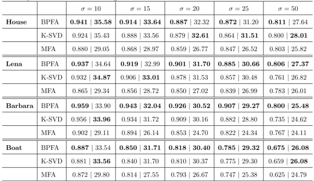
Table 2.1: SSIM |PSNR performance. K-SVD sees the ground truth when choosing the number of dictionary elements for each image.
σ= 10 σ= 15 σ= 20 σ= 25 σ= 50 House BPFA 0.941|35.58 0.914|33.64 0.887|32.32 0.872|31.20 0.811|27.64 K-SVD 0.924|35.43 0.888|33.56 0.879|32.61 0.864|31.51 0.800|28.01 MFA 0.880|29.05 0.868|28.97 0.859|26.77 0.847|26.52 0.803|25.82 Lena BPFA 0.937|34.64 0.919|32.99 0.901|31.70 0.885|30.66 0.806|27.37 K-SVD 0.932|34.87 0.906|33.01 0.878|31.53 0.857|30.48 0.761|26.82 MFA 0.865|29.34 0.856|28.72 0.850|27.02 0.839|26.99 0.783|26.01 Barbara BPFA 0.959|33.90 0.943|32.04 0.926|30.52 0.907|29.27 0.800|25.48 K-SVD 0.956|33.96 0.934|31.72 0.909|30.16 0.882|28.80 0.735|24.62 MFA 0.902|29.11 0.894|26.14 0.853|24.70 0.822|24.34 0.767|24.11 Boat BPFA 0.887|33.54 0.850|31.71 0.818|30.40 0.785|29.32 0.675|26.08 K-SVD 0.881|33.56 0.840|31.70 0.810|30.37 0.775|29.30 0.659|26.08 MFA 0.872|29.80 0.814|27.55 0.793|26.67 0.747|25.38 0.625|24.79
2.4
Experiments
We consider two problems: image denoising and compressed sensing for MRI, which is an application of image denoising. Our experiments show the benefits of PrOMP in the BNP dictionary learning setting compared with K-SVD, the classic dictionary learning algorithm, and also compared with the superior MCMC technique, but applied to an empirically worse inference approach to the same model.
2.4.1 Image Denoising
We compare BPFA using PrOMP with K-SVD [2] and mixtures of factor analyzers (MFA) [49] on an image denoising task. All algorithms performed better than total variation denoising [52], which we omit for space. We observe that BPFA is a Bayesian nonparametric extension of K-SVD that uses OMP instead of PrOMP. MFA is a mixture of non-sparse dictionary learning models (i.e.,z is removed) where each signal chooses one model.
2.4.1.1 Setup
We use four classic test images shown in Figure 2.1. To each image, we add white Gaussian noise with standard deviation σ ∈ {10,15,20,25,50}. To quantitatively assess performance, we use the Structural Similarity Index Measure (SSIM) and PSNR [134] of the denoised image to the ground truth. For K-SVD, we use the code provided by [2] and set the dictionary size to give the best results (more discussed later). In all algorithms, we use the technique in [83] to set the noise parameter. To set the parameters for MFA, we follow the suggestions of [49]. Therefore, all the algorithms are compared under the same noise assumption, which we observed was close to the ground truth. For BPFA, K-SVD and MFA, we extracted 16×16 patches from each image using shifts of one pixel, which overall produced the best results for all algorithms compared with 8×8 and 12×12. We ran the algorithms with the following settings: For BPFAK = 256 and K-SVD K= 200. (Figure 2.2 shows that BPFA used less than 256 elements.). We set η= 2552 and for MFA we set the mixture size to M = 50 and D= 20 to be the subspace size of each mixture.
Figure 2.1: Denoising images: House, Lena, Barbara, Boat.
2.4.1.2 Denoising results
In Table 2.1 we show quantitative results for image denoising. We see that the sparse coding algorithms perform similarly, but overall augmenting with BPFA improved the denoising result over K-SVD. We notice that MFA performs significantly worse than the dictionary learning meth-ods, which shows the advantage of sparse coding versus clustering. However, a key observation is that since K-SVD is not a BNP model, all initialized dictionary elements will be used by the model. Here the number of dictionary elements set for K-SVD changes according to the best result. In practice this would require cross-validation, which is more difficult than our unrealistic approach, which allowed K-SVD to compare with the ground truth when setting this value. We attribute the improvement of BPFA over K-SVD at its best setting to the additional probabilistic structure of the model.
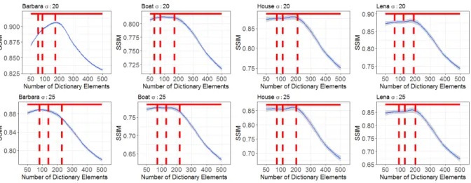
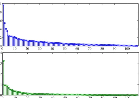
To emphasize this, in Figure 2.2, we show the SSIM results for K-SVD and BPFA for different images and noise settings as a function of dictionary elements set for K-SVD. The results for K-SVD are shown in blue with shaded uncertainty calculated over 20 random initializations. The solid red line shows performance of BPFA. Since BPFA learns the number of dictionary elements we indicate this number with red dashed lines. As it evident, the performance of K-SVD is highly influenced by the number of elements chosen for the dictionary.
Figure 2.2: (Blue: K-SVD, Red: BPFA) Average SSIM results for different images and noise settings as a function of number of dictionary elements for K-SVD, each repeated for 20 trials. The red line indicates the results for BPFA which is not a function of the x-axis. The dashed red lines are the number of dictionary elements in BPFA responsible for representing 95%, 97% and 99% of all input data.
2.4.2 Compressed Sensing MRI
Magnetic resonance imaging (MRI) is a widely used non-invasive medical imaging method that provides high resolutions images from the anatomy [84]. However, its data acquisition process is slow due to physiological and hardware constraints. The data is produced sequentially in the Fourier measurement domain called k-space, and one way to speed up the process is to undersample from this space. However, this violates the Nyquist theorem, and causes aliasing effects in the reconstructed image when the missing values are replaced with zeros. Compressed sensing has had a major impact on MRI (CS-MRI) and allowed for signal reconstruction from very few samples if the signal is sparse in a particular transform domain [84].
Sparse dictionary learning aims learn this transform domain for CS-MRI directly for the data being considered [24, 107]. Let xn ∈ Cd be a patch of an MR image X in a vectorized form. Let F ∈Cu×d be the undersampled Fourier encoding matrix and y=FX∈
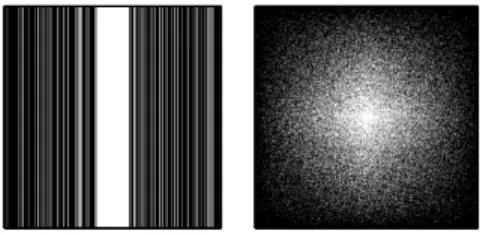
Figure 2.3: Two masks considered. Left: 1D Cartesian sampling with random phase encodes (30% sample rate shown); Right: 2D random sampling (25% sample rate shown).
the sub-sampled set ofk-space measurements. The goal of CS-MRI is to estimate X from the small fraction ofk-space measurements y. The dictionary learning approach to this optimization problem is to find a dictionary W as well as sparse representation sn for each xn such that
xnuWsn and FXb ≈y, with Xb the dictionary learning reconstruction of X.
[64] consider BNP dictionary learning for this task using BPFA, and show that this outper-forms a similar method based on K-SVD [107]. That paper uses MCMC sampling for dictionary learning, which technically should give better results than EM for the same model. However, a major drawback of MCMC, as well as the variational inference approach of [95], is that updating each dimension ofznis conditioned on the current values of the other dimensions. This can lead
to slow mixing, i.e., bad local optimal solutions, because selecting a dictionary element depends on which other elements are currently selected. PrOMP for BPFA (and OMP for K-SVD) are fundamentally different in their sparse coding in that all elements are initialized to zero and greedily selected. We compare this PrOMP version of BPFA with the MCMC sampler used by [64] to illustrate that this greedy EM approach to dictionary learning improves the MCMC approach, which is state-of-the-art for this BNP model.
We experiment on two publicly available 512×512 MRI of a shoulder and lumbar. We apply the masks in Figure 2.3 to subsample MRI in the Fourier domain. We consider various sampling rates for each mask and different sample noise settings. Figure 2.4 shows one example of the reconstruction replacing the missing values with zeros. For all images, we extract 6×6 patches and set other parameters according to [64].
It is well-known that CS inversion is closely related to image denoising, with the noise due to image artifacts from subsampling; [64] provide a discussion on this in the context of dictionary
Figure 2.4: (left) Original Shoulder, (middle) Shoulder distorted by Cartesian 35% mask, (right) Shoulder distorted by Cartesian 35% mask and noise with σ= 0.05.
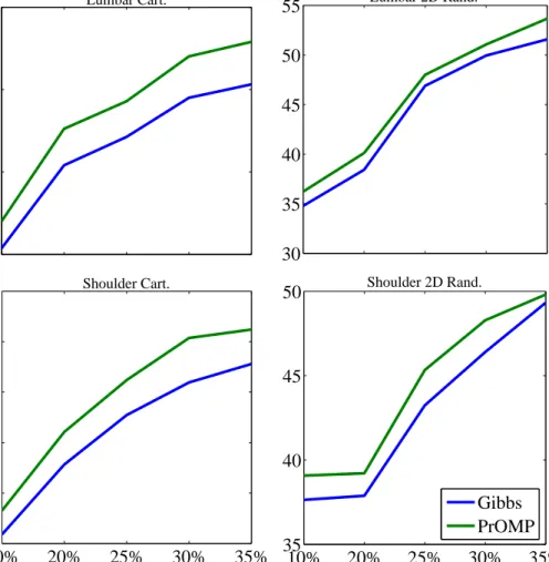
learning for CS-MRI. Therefore, comparing PrOMP-EM with MCMC for CS-MRI is essentially a comparison of how the denoising abilities of these two inference approaches to the same model translates to a particular task. We first consider the noise-free setting. Figure 2.5 compares the results of PrOMP and MCMC Gibbs sampling for different MRI, masks and sampling percentages. It is evident that PrOMP performs better at reconstructing original image. We also evaluate performance on the same setup, but with additive sampling noise with standard deviationσ = 0.05. (The original MRI was scaled to [0,1]. Other settings ofσ showed the same pattern.) For these experiments we use the original noise-free MRI as ground truth. Figure 2.6 shows the PSNR results for lumbar image for different masks, sampling percentages and noise values. It is evident that PrOMP performs better in reconstructing the original image as well as denoising it. Figure 2.7 shows that PrOMP is capable of learning a sparser representation than MCMC with far fewer dictionary elements required.
2.5
Conclusion
I proposed probabilistic orthogonal matching pursuit (PrOMP) for sparse data representation. Our probabilistic approach extends orthogonal matching pursuit (OMP), making it suitable for statistical dictionary learning models with Bayesian nonparametric priors. We derived theory for PrOMP similar to that of OMP, and discussed how PrOMP can improve existing dictionary learning models. We evaluated the performance on image denoising and compresses sensing for
30 35 40 45 Lumbar Cart. 30 35 40 45 50 55 Lumbar 2D Rand. 10% 20% 25% 30% 35% 34 36 38 40 42 44
Sampling %
PSNR
Shoulder Cart. 10% 20% 25% 30% 35% 35 40 45 50Sampling %
Shoulder 2D Rand. Gibbs PrOMPFigure 2.5: PSNR results in the noiseless setting for different MRI, masks and sampling percent-ages. PrOMP for EM outperforms MCMC for the same BNP dictionary learning model. magnetic resonance imaging (CS-MRI), showing that PrOMP for BPFA improves the classic K-SVD model, as well as MCMC sampling for the same BNP dictionary learning model.
10% 20% 25% 30% 35% 26 28 30 32 34 36 Sampling % PSNR 10% 20% 25% 30% 35% 29 30 31 32 33 34 Sampling % Gibbs PrOMP
Figure 2.6: PSNR results with additive sampling noise (σ = 0.05) for the lumbar MRI, using the Cartesian (left) and Random (right) masks and different sampling percentages. PrOMP outperforms MCMC for the same BNP dictionary learning model.
0 10 20 30 40 50 60 70 80 90 100 0 0.2 0.4 0.6 0.8 1 0 10 20 30 40 50 60 70 80 90 100 0 0.1 0.2 0.3 0.4
Figure 2.7: Stem plots of πk (sorted) for lumbar MRI with Cartesian 25% sampling mask.
PrOMP (bottom) shows the expectation and MCMC (top) shows the best performing iteration. PrOMP learns a much sparser representation for this model.
Chapter 3
Beta Process Subspace Analysis
In this chapter, I present a new model for latent subspace analysis in which the number of subspaces and dimensionality of each subspace are inferred using Bayesian nonparametric priors [41]. Latent membership models enable us to discover underlying structures in a dataset where in this chapter the latent members are subspaces.In our formulation, a beta process prior allows for an unbounded number of subspaces, while gamma process priors on the variances of dictionary elements in each subspace allow for unbounded subspace dimensionality. We call our modelbeta process subspace analysis (BPSA), which can be thought of as a subspace extension of a related factor analysis model that uses the beta process. We derive a scalable EM algorithm and demonstrate performance on image denoising tasks and learning on large image dataset.
3.1
Introduction
Latent membership models are useful techniques in discovering and describing underlying structure in a dataset. Latent members of the model are designed such that each observation can be constructed from those members. In this work we focus on learning these latent members in the format of a dictionary that consists of subspaces, as well as sparse coding for the observations using dictionary subspaces.
Sparse coding seeks to decompose a signal into a combination of a small subset of patterns selected from the dictionary. The goal of dictionary learning is to simultaneously learn these
patterns in the dictionary and the sparse representation of the signals [2]. Bayesian nonparametric (BNP) models based on the beta process prior represent one approach to this problem in which model selection parameters such as dictionary size are inferred directly from data [55, 71, 95, 140]. In such models, an infinite collection of beta priors constitute prior distributions on the activation probabilities of a corresponding infinite collection of dictionary elements; Bayesian nonparametric analysis ensures that a finite data set generated from a Bernoulli process will use a finite, but random number of these dictionary elements with probability one.
Typically, sparsely coding data with a dictionary entails learning which dictionaryvectors a signal possesses [2, 71, 95]. Previous works have further used it in classifying images [4, 105, 136] and in encoding data with linear dynamical systems [63]. To a lesser extent, previous work has also been done on representing signals with latent subspaces [22, 49, 65, 77]. This generalization allows for groups of signals to be learned such that dictionary elements within the same subspace capture correlated structure within the signal. Such a representation can result in a more precise and efficient signal representation. Independent subspace analysis (ISA) [65] and mixtures of factor analyzers (MFA) [49] represent two approaches; in ISA, signals are represented as linear combinations of multiple weighted subspaces, while with MFA a signal is assigned via a mixture on subspaces to a single factor analysis model.
In the same spirit that has motivated BNP extensions to factor analysis, MFA and ISA are restricted by the fact that the number of subspaces and the dimensionality of each subspace must be defined in advance. In this work we aim to address these shortcomings using BNP priors. Specifically, we propose a beta-Bernoulli process for sparsely coding signals viasubspaces, while we define gamma process priors on the variances of the Gaussian priors on dimensions in each subspace; posterior inference of the first prior learns the number of subspaces, while inference for the second prior learns the dimensionality of each subspace. We observe that in our model definition, each subspace can have a different dimensionality, which has a significant advantage of side-stepping the combinatorial and local-optima problem this would present for cross-validation.
We refer to our proposed model asbeta process subspace analysis (BPSA). We develop a new scalable EM-based algorithm along the lines of other scalable dictionary learning approaches [87, 114, 115]. Our scalable algorithm can be viewed as a special case of stochastic variational
inference [19, 61]. We show that BPSA is a competitive method for nonparametric dictionary learning on a denoising problem [115, 140].
3.2
Beta Process Subspace Analysis
We propose beta process subspace analysis (BPSA) for nonparametric dictionary learning. We assume that we have a set of signals x={x1, . . . ,xN}, wherexn∈Rd. We model these vectors as Gaussian random variables in which the mean vectors are represented hierarchically as follows. For fixed and large integer valuesK and D, first generate global variables
wki |ηik ∼ N(0, ηkiId), ηki ∼ gamma( δ D,1), πk ∼ beta αγ K, α(1− γ K) . (3.1)
The index values arei= 1, . . . , D andk= 1, . . . , K. Parameters α, γ, δ >0 are positive and set such thatαγ K andδ D. The vector wki ∈Rd corresponds to the ith dimension vector of thekth subspace andId indicates ad-dimensional identity matrix. In principal, we can let
K, D→ ∞, but for inference purposes we let them be finite, but large integer values. Let Wk
be the set of allwik for a particulark organized in a d×D matrix. In the limit K → ∞ the random measure HK =PKk=1πkδWk constructed from these random variables converges to a
beta process, and the larger the value ofK the more accurate the approximation. Similarly, the random measure Gk
D = PD
i=1ηkiδwi
k converges to a marked Poisson process asD→ ∞ with the
measures following a gamma process. We note that a well known property of these two priors is that only a small number ofWk will haveπk > for all >0, and similarly only a small number
ofηki > for a fixedk. We make a more precise statement about these asymptotics for BPSA in Proposition 3.1 below.
For each patchxn, sparse coding then proceeds as follows. First, independently generate
Then, the nth observation xn is drawn xn∼N XK k=1 znk(Wkckn), σ2Id . (3.3)
Sparsity dictionary learning is enforced by the beta prior on eachπk. This prior on πkencourages
znk = 0 for eachn over all but a small number of values of k. Sparse coding results from the
values of k for whichπk is large, but still allows for factors to turn on and off according to the
Bernoulli process. Though the limit asK, D→ ∞ is a doubly-infinite sum of weighted vectors, the following proposition shows that xnhas finite magnitude almost surely.
Proposition 3.1. For a vectorxn generated by BPSA, kxnk2 <∞ almost surely as K, D→ ∞.
Proof 3.1. We analyze this in the known beta and gamma process limits, rather than asymptot-ically. We use the facts thatE[kxnk22]<∞ implies E[kxnk2]<∞, and for a vectorv∼N(µ,Σ),
the expected squared norm is E[kvk22] =µTµ+ trace(Σ). We define the sets F1 ={W,zn,cn}
andF2 ={π,η}. Suppressing some conditioning on the RHS, by the tower property we have
E[kxnk22] =E[E[E[kxnk22|F1]F2]] (3.4) =E kP∞ k=1znk P∞ i=1c k niwki k2 2 +dσ2 =P∞ k=1E[znk] P ∞ i=1E[(c k ni)2]E[kwkik 2 2] +dσ2 =P∞ k=1E[πk] dP∞i=1E[ηik] +dσ2 =d(δγ+σ2). The value P∞
i=1E[ηki] =δ is the expected total measure of a gamma process with parameters δ
and 1, while P∞
k=1E[πk] =γ is the expected total measure of a beta process with parameters α
andγ. The result follows from Chebyshev’s inequality.
3.3
Example: Tiny Images
We show an illustrative example of what BPSA learns on the 80 million tiny images dataset [126]. Each color image is 32×32×3 in size, giving a vectorized dimensionality of d= 3072. For this problem we initialized the model to K = 100 subspaces, each ofD= 10 dimensions. We
randomly initialized the dictionary and ran the scalable inference algorithm described in Section 3.4. In this experiment we were able to process almost of of the images with the algorithm seeing each of these images one time. The algorithm inferred 24 subspaces in this time, pruning away the remaining 76. The number of learned vectors inside each subspace varies between 1 to 9.
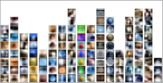
Figure 3.1: Final dictionary learned on Tiny images dataset. Each column represents a subspace and each learned vector of a subspace is reshaped to be shown by an image. From left to right, subspaces are ordered to show the most used to the least used ones in image representation.
Figure 3.1 shows the final learned dictionary. Each column shows a dictionary subspace, and vectors in subspaces are shown as 32×32×3 images. We show the 17 most-used subspaces in this figure (24 were learned in total). These subspaces are shown ordered by their probability of usage from left to right. We scale the vectors of each subspace to better visualize see the learned patterns inside each subspace. It can be observed that our nonparametric model has learned only a portion of the vectors inside each subspace and pruned away the remaining.
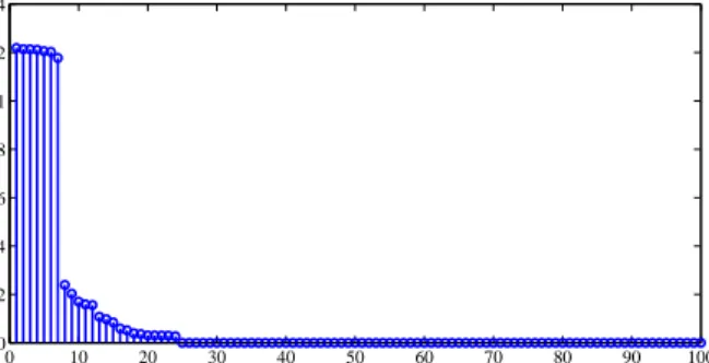
Figure 3.2 shows the ordered probability of using each dictionary subspaces. We notice that only 24 subspaces are learned, while the remaining 76 subspaces have been pruned out by virtue of their having zero probability (i.e., not being used by data).
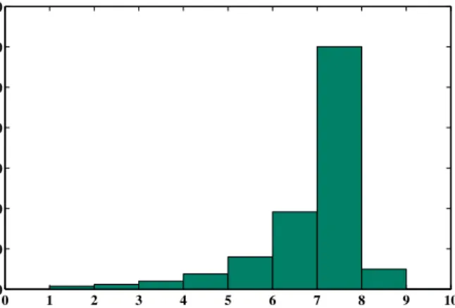
Finally, we randomly selected 100,000 images to investigate how many dictionary subspaces they use in their final representation. In Figure 3.3 we show a histogram of the number of used
0 10 20 30 40 50 60 70 80 90 100 0 0.02 0.04 0.06 0.08 0.1 0.12 0.14
Dictionary Elements (subspaces)
Probability
Figure 3.2: Probabilities of using each dictionary subspace in representing images ordered form the most probable to the least.
subspaces for representing particular images. As seen, almost 60,000 images used 8 subspaces in their representation, with all images using less than 9 total subspaces. Simpler images required significantly fewer subspaces. This initial experiment supports our goal in developing BPSA to nonparametrically and simultaneously learn a sparse set of varying-dimensional subspaces for data representation.
3.4
Inference for BPSA
We derive a MAP-EM algorithm for BPSA that uses a marginalization trick similar to MFA, with the result being similar to the sparse coding algorithm used by K-SVD. We then present a scalable approach for inference using stochastic optimization. We learn point estimates for each Wk andzn, and conditional posterior q distributions on all other model variables. The
conditional independence induced byWk and zn is what makes this an exact EM algorithm,
rather than a mean-field variational approximation using delta-functionq distributions on Wk
and zn (see discussion below).
Let x,z,c,π,η andW indicate sets of all of the respective variables and data. In EM for BPSA, the goal is to maximizep(x,z,W) over the sparse coding vectors zn and subspaces Wk
0 1 2 3 4 5 6 7 8 9 10 0 10,000 20,000 30,000 40,000 50,000 60,000 70,000
Number of used subspaces in coding
Figure 3.3: A histogram of number of subspaces used in representing 100,000 randomly selected images.
hidden variables and set up the EM objective function on the log marginal distribution, lnp(x,z,W) = Eq h lnp(x,z,W,c, π, η) q(c, π, η) i | {z } L(z,W) + Eq h ln q(c, π, η) p(c, π, η|x,z,W) i | {z } KL(qkp) . (3.5)
The conditional posterior distribution factorizes nicely, and so we have an exact forms forq(c, π, η) that mirrors the factorization
p(c, π, η|x,z,W) | {z } q(c,π,η) = QNn=1p(cn|xn,zn,W) | {z } q(cn) × QKk=1p(πk|z) | {z } q(πk) QK k=1 QD d=1p(ηik|wik) | {z } q(ηi k) . (3.6)
All three of the distributions above are in closed form and are in the Gaussian, beta and generalized inverse Gaussian families, respectively. We can update each factorizedq in this way to locally optimize Eq. (3.5) overz and W.
3.4.0.0.1 Connection to variational inference. We can re-frame the MAP-EM objec-tive function of Eq. (3.5) as variational inference by using delta-function q distributions on z and W. In this case, defining the factorization q(c, π, η,z,W) = q(c, π, η)δzδW and writing
p(c, π, η,z,W|x) =p(c, π, η|x,z,W)p(z,W|x), we can derive a variational inference algorithm that is identical to the MAP-EM algorithm described below. The choiceq(W) =δW is reasonable
because the posterior is tied to the data size; with large data sets, or even large individual images, a Gaussianq(W) would be a highly peaked distribution. The other natural choice forq(z) is a set of Bernoulli distributions, as used in [95, 115], but since this effectively acts as a second weight on the dictionary elements, it can lead to scaling issues when combined withq(c). We therefore believe that 0–1 sparse coding forznand allowingq(cn) to capture all weight information is more
appropriate, and so q(z) =δzis a good choice.
3.4.1 Sparse coding EM step
We break the algorithm into two parts: In the first part, we derive a greedy algorithm for jointly learningzn andq(cn). This sparse coding step is not as straightforward as it might appear, since
ifznk = 0, then the corresponding updatedq distribution oncknwill revert to the zero-mean prior,
which makes it effectively impossible to setznk = 1 in the following iteration after computing the
E-step overck
n. To mitigate this, we can integrate out cn when learningzn. We first observe that
lnp(x,z,W) can be directly optimized greedily over z, which would be one approach. However, updatingW is not in closed form here. Since Eq. (3.5) is an equality, one solution is to iteratively (i) update the LHS of (3.5) over z, and then (ii) update the RHS of (3.5) over W and all q
distributions.
We define a similar greedy algorithm, where instead of fully optimizing each zn on the LHS
of (3.5) and then updating the fullq(cn) on the RHS, we construct asequence of EM equalities.
Since the joint likelihood factorizes overxn the objective sums over each data point and so we
can sparsely code each observation independently. We can marginalize out arbitrary subsets of dimensions ofcn to equivalently write
lnp(xn,zn|W) = Eq h ln p(xn,zn,cnA, π|W) p(cnA|xn,zn,W)p(π|z) i = Eq h ln p(xn,zn,cnA, c j n, π|W) p(cnA, cjn|xn,zn,W)p(π|z) i , (3.7) for a particular observation xn and current sparse coding vector zn and using the following
definitions: A ⊂ {1,2, ..., K}, j /∈ AandcnAdenotes the subset ofcn corresponding to subspaces
indexed by A. We have also compressed the EM equality of Eq. (3.5) on the RHS side for space. What the equality in Eq. (3.7) shows is that we can arbitrarily integrate out portions of the vector cn corresponding to subspaces for whichznk = 0. Let A={k:znk = 1}, the set of
Algorithm 3 Sparse coding greedy EM algorithm 1: input:DictionaryWandq(πk) =p(πk|z1, . . . ,zN).
2: output: Sparse codingznandq(cn) (index ignored)
3: foreach patchxdo
4: Setz= 0 and index setA=∅ 5: For allj, initialize
ξ+j = lnp(x|W, zj= 1) +Eq[lnπj]
ξj− = lnp(x|W, zj= 0) +Eq[ln (1−πj)]
6: whilemaxj ξj+−ξ
−
j > 0do
7: Setj0 = arg maxjξ
+
j −ξ
−
j (see Eq. (3.9))
8: AugmentA ← A ∪ {j0}. Setzj0= 1 andξj+=−∞ 9: Updateq(cA) =p(cA|x, z, W) (see Eq. (3.10))
10: For allj /∈ A, update
ξ+j = Eq[lnp(x|cA,W, zj= 1)] +Eq[lnπj],
ξj− = Eq[lnp(x|cA,W, zj= 0)] +Eq[ln (1−πj)]
11: end while
12: end for
active subspaces for observationn. (We will ignore the indexn from now on.) Then our two step greedy procedure (i) calculates the marginal log likelihood in Eq. (3.7) using the equality in the first row, picking the subspace with indexj that increases this value the most, and then (ii) increments the setAby adding indexj, sets the corresponding dimension ofz to one and recomputes the log marginal likelihood using the equality on the second row of Eq. (3.7). This augmented set then is redefined to be the first row and the procedure continues by expanding over new dimensions ofcn. If no subspace increases the marginal likelihood, then sparse coding
terminates. In this way, the Bayesian approach provides an automatic means for determining the number of subspaces appropriate for each observation.
The outline of the greedy sparse coding algorithm is given in Algorithm 1. Using the sequence of equalities constructed as in Eq. (3.7), this algorithm can be shown to monotonically increase the objective in Eq. (3.5) using the standard EM proof.
3.4.1.0.2 Procedure: As mentioned, each step of the sparse coding algorithm consists of two parts: determining which new subspace to add (or terminating) and then recomputing the log marginal likelihood using a new latent variable expansion via EM. To determine which subspace to add, we compute as a score the amount of increase in the objective function in Eq. (3.5) from adding each potential subspace. In Algorithm 1 we refer to this score asξ+j −ξ−j , whereξ+j is the objective function using subspacej and ξj− not using it. Again suppressing observation indexn, the likelihoods used in this calculation are
p(x|cA,W, zj = 1) = N(x|Pk∈AWkck, σ2I+WjWTj),
p(x|cA,W, zj = 0) = N(x|Pk∈AWkck, σ2I).
(3.8)
Letq(cA) =N(cA|µA,ΣA) and define the residual of the approximation given the active set
A to be rA = x−Pk∈AWkµk. Using the matrix inversion lemma and defining the stacked
matrixWA= [Wk]k∈A, the score of subspacej equals
ξj+−ξj− = 1 2σ2r T AWj(σ2I+WjTWj)−1WTjrA + 1 2σ2tr{W T AWj(σ2I+WTjWj)−1WTjWAΣA} −1 2ln|Id+σ −2W jWjT| + Eq[lnπj] − Eq[ln(1−πj)]. (3.9)
The expectationsEq[lnπj] and Eq[ln(1−πj)] are in the next section. The parameters ofq(cA)
are
ΣA= (I+σ12WATWA)−1, µA = σ12ΣAWATx. (3.10)
These are of size D|A| ×D|A| and D|A| ×1, respectively. Parsing Eq. (3.9) shows that the score measures how correlated subspacej is with the residual, and takes into account the prior probability of subspacej, as well as two other probabilistic factors. The running time of this algorithm is comparable to orthogonal matching pursuits.
3.4.2 Dictionary EM steps
After sparse coding the vectors xn withzn, we run EM on cn,η and each Wk, and update the
accumulated during the sparse coding step, it is limited by the matrix inversion in Eq. (3.13) below