2-D inversion of VES data in Saqqara archaeological area, Egypt
Gad El-Qady, Chika Sakamoto, and Keisuke Ushijima
Engineering Geophysics, Faculty of Engineering, Kyushu University, 36 Hakozaki, Fukuoka 812-8581, Japan (Received October 14, 1998; Revised August 16, 1999; Accepted August 23, 1999)
The interpretation of actual geophysical field data still has a problem for obtaining a unique solution. In order to in-vestigate the groundwater potentials in Saqqara archaeological area, vertical electrical soundings with Schlumberger array have been carried out. In the interpretation of VES data, 1D resistivity inversion has been performed based on a horizontally layered earth model by El-Qady (1995). However, some results of 1D inversion are not fully satisfied for actual 3D structures such as archaeological tombs. Therefore, we have carried out 2D inversion based on ABIC least squares method for Schlumberger VES data obtained in Saqqara area. Although the results of 2D cross sections were correlated with the previous interpretation, the 2D inversion still shows a rough spatial resistivity distribution, which is the abrupt change in resistivity between two neighboring blocks of the computed region. It is concluded that 3D interpretation is recommended for visualizing ground water distribution with depth in the Saqqara area.
1.
Introduction
Inversion of geophysical data involves the estimation of the parameters of a postulated earth model from a set of observed data. It may be viewed as an attempt to fit the re-sponse of an idealized subsurface earth model to a finite set of observed data. With the increased availability of faster computers, it is now practical to employ numerical model-ing techniques to invert resistivity data for a 3D geological structure. However, there has been no great success in over-coming the uniqueness problem associated with the practical; that is uncertain, incomplete, geophysical data. The Monte Carlo method, in which a huge number of randomly gener-ated models are tested against the data, has been used for resistivity soundings data (Strenberg, 1979) in an attempt to characterize all models which agree with the observations. Such computations can never be exhaustive, and even cal-culation ranging over the class of simple layered models is computationally extravagant in the light of the insight ob-tained from them. The best policy may be to seek a model whose features are in some way essential characteristics of any of the possible solutions, one of which presumably is the true structure, (Vozoff and Jupp, 1975; Constableet al., 1987).
However, the dimensionality of the earth’s model should be based on the general characteristics of the geology within the survey region. This dimensionality is often to be deter-mining simply by the availability of the interpretation tech-niques. Whatever, the basic motivation for seeking smooth model is that we do not wish to be misled by features that appear in the model but are not essential in matching the observations.
In this study, we carried out 2D inversion using the algo-rithm proposed by Uchida (1991). Since the forward
prob-Copy right cThe Society of Geomagnetism and Earth, Planetary and Space Sciences (SGEPSS); The Seismological Society of Japan; The Volcanological Society of Japan; The Geodetic Society of Japan; The Japanese Society for Planetary Sciences.
lem of electrical and electromagnetic fields for a given earth model is usually non-linear problems, we have to linearize the problem by a certain assumption to perform the least squares inversion. A Jacobian matrix, consisting of partial derivatives of the data with respect to the model parameters, is often ill conditioned; hence the direct solution of the ma-trix provides a non-realistic rough resistivity model of a large oscillation.
2.
Theoretical Basis
Here in this algorithm, we consider a two-dimensional earth model whose resistivity varies along thex- andz-axis and doesn’t change alongy-axis. Since the current is injected at a point source on the ground surface, however it flows three dimensionally in the earth. The response in a 2D earth is given by Poisson’s equation as:
− ∇ ·[σ(x,z)∇V(x,y,z)]=I(x,y,z), (1)
whereσ(x,z)is the conductivity,V(x,y,z)is the electric potential and I(x,y,z)represents the current source inten-sity. By applying the Fourier transform to Eq. (1) with respect to theycoordinate, we obtain:
−∇[σ(x,z)∇ ˆV(x,ky,z)]+kyσ (x,z)Vˆ(x,ky,z)
= ˆI(x,ky,z), (2)
whereˆmeans the Fourier transform andky is the Fourier transform variable. A detailed explanation of the finite el-ement discretization of Eq. (2) is given in Sasaki (1981). Discretization over mesh yields a matrix equation,
K V =S (3)
whereK is aL ×L sparse band matrix with positive sym-metric values. This is determined by the geometry and con-ductivity of each finite element, L is the number of nodes,
V is a column vector of the unknown potential at each node,
1092 G. EL-QADYet al.: 2-D INVERSION OF VES DATA andSis the column vector of current source intensity at each
node. The potentialVin real 3D domain can be obtained by solving Eq. (3) and applying inverse Fourier transform,
V(x,0,z)=(1/π)
∞
0
ˆ
V(x,ky,z)dky, (4)
and the apparent resistivity for Schlumberger can be calcu-lated as:
ρa = GV
I , (5)
whereGis the geometrical factor, andV is the calculated potential difference between the receiving electrodes,Mand
N.
If we let(Pi)be 2D model’s parameters,(ρa j)be appar-ent resistivities,(φ)the misfit between the observed and the theoretical apparent resistivities. The improvement of pa-rameters of the model should be expressed in a logarithmic scale as:
xi =logPi, i =1, . . . ,m
yj =logρa j, j =1, . . . ,n (6) where: m, is the number of model parameters, andn, is the number of the observed data.
Here we describe the 2D model, which holds its block boundaries during the inversion and only the resistivity within each block changes with the iteration procedure. The misfit(φ)of the data is determined by the equation:
φ= 1
j)is the calculated data. If we consider the(k−1)-th iteration of the inversion process, applying the Taylor expansion toyj(x)atx(k−1)and
neglect the terms of the second and higher order we obtain:
yj(x(k))=yj(x(k−1))+
where the superscript(k)meansk-th iteration. In order to minimize the misfitφ, the condition ∂∂φx
i =0 should be
sat-isfied. Furthur explanation was descried by Uchida (1991). In order to judge the convergence, a statistical criterion, ABIC (Akaike Bayesian Information Criterion) has been pro-posed by applying the maximum entropy theorem to the Bayesian statistical (Akaike, 1980). This ABIC works as an index to determine the maximum likelihood of the model. A smaller ABIC indicates a larger likelihood and entropy, hence gives a best model. The model is obtained under the assumption that the data error and roughness (spatial deriva-tives of the parameters) are normally distributed with zero-mean. The optimum smoothness is also obtained in the pro-cess of the likelihood maximization.
For the least-squares inversion with smoothness regular-ization, we seek a model, which minimizes both the data misfit and model roughness. From a statistical point of view, the Bayesian procedure can be applied for this purpose by taking the smoothness constraint as a prior distribution of the model parameters (Jackson and Matsura, 1985). One of
the advantages of this method is that we do not always re-quire information on individual measurement error to judge the convergence. Also, the selection of an optimum smooth-ness is completely objective. According to Akaike (1980), bayesian likelihood can be expressed as follows:
L(m/d)=
p(d/m)π(m)dm, (9)
where,p(d/m)is the probability density function of the data, which is called the data distribution, andπ(m)is a prior dis-tribution. In Bayes’rule, we assume that the model is based on a priori information, such as a smoothness constraint or a parameter constraint, and that its probability density function isπ(m). It is supposed that the model which maximizes the bayesian likelihood in Eq. (9) makes the average logarithmic likelihood maximum. ABIC is derived to provide an index for finding the maximum Bayesian likelihood and defined by:
ABIC=(−2)log(maxL(m/d))
+2 dim(hyperparameter) (10)
wheredis a set of observed data and a hyperparameter means a parameter, which is not used to express the model directly, but is used to obtain parameters of the model. The only hyperparameter in this case is the smoothing parameter(α), further explanation of the equations was described by Uchida (1993), then ABIC can be written as:
ABIC(α)=nlog is a hypothetical model,W, is a diagonal weighting,U is a function defined as:
U =misfit+roughness penality of the model = W d−W F(m)2+α2Cm2, (12)
C, is a roughness matrix of a model parameter, which gives thefinite difference of the model parameters between later-ally and verticlater-ally adjacent blocks in the mesh, and F is a non-linear forward function which works on the model to obtain the response.
As well as the optimum smoothness is judged by minimiz-ing ABIC, we have to consider weighted root mean square misfit as well as another misfit parameter called u-rms. This u-rms misfit is defined as:
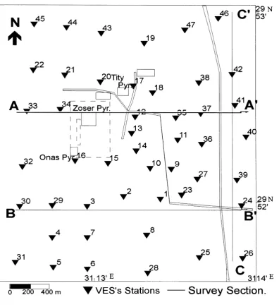
Fig. 1. Location Map for Geophysical survey in Saqqara area.
which extends between Saqqara plateaus and the Nileflood plain and the plateau, where Saqqara pyramids are found.
Lithostratigraphically, the shallow geologic section of Saqqara area composed of Quaternary deposits which com-prises of river terraces of sands and gravel with a thick-ness varying between 30 to 180 m. These were underlined by gravel units (10 m) of Pleistocene, which underlined by Pliocene formations. Pliocene rocks are varying in compo-sition from limestone to marl and sandstone with total thick-ness about 23 m. This unit overlaps the Eocene formations with angular unconformity. Eocene rocks are represented by a sandy to marly yellow limestone. These rocks uncom-formably lie over the Cretaceous limestone rocks.
4.
Data Analysis and Interpretation
In this work, forty-seven vertical electrical soundings (VES) were conducted in a grid pattern aiming to map the groundwater aquifer in Saqqara area (Fig. 1). The well-known Schlumberger configuration of AB/2 starting with 1 meter up to 300 meter in successive steps was applied.
At few stations measurements were found convenient to be ended before 300 m. The distance between stations varies between 300 and 500 meter according to the topography, land feasibility and the applicability of the array. A 1D interpreta-tion had been done by (El-Qady, 1995) using Zohdy’s (1989) method. The main resistivity regime is of the type AAHA (ρ1 > ρ2 > ρ3 > ρ4 < ρ5 < ρ6) and their lithologies
vary between gravel, marly sand, sandy clay, saturated sand and limestone respectively. The form of the results automat-ically reflects the locations and the electrical properties of relevant layers buried in the earth. The method is robust and requires no external information on the number of high and low of the resistivity function. So, it is important to under-stand how and to what extent 1D approximations represent the true structure. This will be done using multidimensional inversion methods such as 2D or 3D.
1094 G. EL-QADYet al.: 2-D INVERSION OF VES DATA
Fig. 2. Shematic view of the calculation mesh.
mesh parameters to be compatible with our AB/2 distances (Fig. 2). That is one of the advantages of this algorithm that we can handle almost three decades of AB/2 with a single calculation mesh. In the forward calculation, the current electrodes were put near the center point and potential elec-trodes at outer position. In this case, due to the reciprocity theorem, apparent resistivity for all AB/2 of all the sounding can be obtained by one forward calculation.
4.1 Inversion results
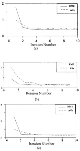
As we seek a model which minimizes both the data misfit and model roughness, and whenever the selection of an op-timum smoothness is completely objective. So, we have to run the inversion process until the bestfit is attained. The program outputs 7 models per iteration, accompanied by 7 values for all the inversion parameters. Then it selects the best model according to the smoothing factor and rms-misfit as an initial model for the next iteration. Figure 3 represents rms- misfit and the smoothing parameter(α)as a function of the iteration number for the profiles A-A’, B-B’and C-C’
respectively. It is obvious that both of rms. andαnearly con-verge with a similar manner; decrease as iteration proceeds. We can judge that, after thefifth iteration, they become nearly stable with minimum values.
Since we have 7 models per iteration, we should investi-gate the behavior of the inversion parameters (ABIC, u-rms, roughness, andα) for each iteration as shown in Fig. 4 for the profile (A-A’). At thefirst iteration, all the inversion param-eters have higher values that indicate a non-smooth model. Whereas the iteration process proceeds, the parameters curve become smaller amplitude and slightly smoother. The deci-sion of the convergence can be done by checking how ABIC decreases as the iteration proceeds. When the convergence is attained, the decreases per iteration become very small as shown in Fig. 4(a). It is obvious that rms. and Urms misfits also converge with a similar manner and attain the minima at the fifth iteration. This is the same with the roughness parameter. Figure 5 shows the inversion parameters as a function of the smoothing parameter (α) at each iteration for the profile B-B’. In thefirst iteration all the parameters have higher values which decrease as the iteration proceeds. Also, the minima of ABIC, rms and Urms misfits are obvious for
Fig. 3. The rms misfit and Alfa as a function of iteration numbers: (a) the profile (A-A’), (b) the profile (B-B’) and (c) the profile (C-C’).
the first three iterations. However, for the all iterations, a rougher model gives a smaller misfit, while the minima of the curve is still clear except for thefifth iteration, it becomes nearly straight line as shown in Figs. 5(a), (b) and (d).
4.2 2D cross sections
Depending on the results and variation of the inversion pa-rameters, we can conclude that the model of thefifth iteration represents the bestfit and minimum ABIC for this data set.
1096 G. EL-QADYet al.: 2-D INVERSION OF VES DATA
1098 G. EL-QADYet al.: 2-D INVERSION OF VES DATA
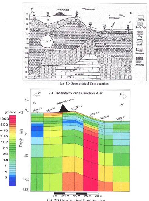
for the inversion was 145 and the number of resistivity blocks is 99 resistivity blocks. The general features of this inverted model; which correlated with 1D cross section are shallow thin resistive layer followed by a conductive relatively thick layer, then a resistive basement. It is obvious that the shal-low section of the eastern part is more conductive. This is due to the presence of cultivated land and Nile silt deposits. This part includes a lenticular moderate resistive layer, which represents the shallow water-bearing unit in the area. How-ever, the resistivity increases as far as depth, where Pliocene and Eocene deposits which are varying in lithology between marl, sandstone and limestone. Except at the VES 34 nearby Zoser pyramid, it has a relatively higher resistivity, which dis-agreed with the neighboring VES stations. However, the 2D respond clearly had been influenced by the expected geolog-ical structure correlated with 1D section. The correlated 2D cross-section still gives an ambiguous interpretation, which may be an archaeological body.
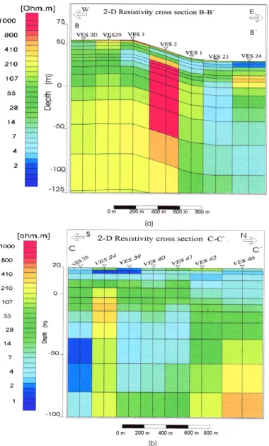
The inverted 2D cross section of the profile (B-B’) which results from the 5-th iteration is shown in Fig. 7(a). The smoothing factor is 0.7, while the number of the observed data is 124 and 117 resistivity block. Inspection of this sec-tion showed that, it has nearly the same geoelectrical structure as profile (A-A’), however the eastern shallow lenticular body became more resistive. This is as well as the high resistivity anomaly around VES 2 became smaller in the size.
Figure 7(b), shows the inverted 2D section of the profile C-C’. It is resulted from 166 data point and 117 resistivity block with smoothing factor 0.3. It is clearly seen that, the cultivated area in the whole profile had affected the 2D re-sponse. This represents a huge thick body of low resistivity. However, there are some spots of moderate resistivity repre-sent the sand lenses of the Nile deposits. We couldfind a little bit mismatch at the intersection of the profile C-C’with both the profiles A-A’and B-B’, although the interpretation gave almost the same geoelectric sequence. This is because the 2D section is greatly affected by the direction of Schlumberger array spreading whether is it parallel or perpendicular to the section.
Investigations of the constructed 2D cross-sections of all the study area and its correlation with 1D section are sum-marized as:
1. Spots of relatively high resistivity values at shallow depth, which may represent shallow gravel, layer.
2. This is followed by a huge thickness conductive body intruded by a relatively moderate resistivity represents the Quaternary Nile sediments. While the moderate resistivity values represent the shallow water-bearing unit in the study area. This, which has the main danger, affected the archaeological sites in the study area.
3. The 2D response had been influenced by the geological structures in the area such as Saqqara plateau and the archaeological bodies in the area.
5.
Conclusion
The present work aims to apply 2D inversion on the Schlumberger resistivity data to elucidate the subsurface
structure and the ground water distribution in Saqqara area. Forty-seven Schlumberger VES were interpreted in terms of 2D cross section using algorithm based on ABIC least squares and utilizefinite element calculation mesh.
The inversion procedure can reduce the misfit through it-erations. However, the resultant cross-section of 2D model often shows a rough spatial resistivity distribution that is, the resistivity changes abruptly between two neighboring blocks, and extraordinary low or high resistivities are ob-tained. Highly correlation has been found between the re-sultant 2D cross sections and 1D-inversion results, however it still gives an ambiguous geologic interpretation. It is clear that the 2D cross section had been affected by spread direc-tion of Schlumberger array as it is appear at the intersecdirec-tion of the profile C-C’with both A-A’and B-B’. So we may recommend the 3D interpretation for visualizing ground wa-ter distribution with depth and to elucidate the subsurface structure of Saqqara area. However, it is recommended to use a different method of 2D analysis, may it gives another solution with a different 2D response.
A reliable inversion technique for an electrical method is essential to meet the requirement for a more detailed delin-eation of underground media.
Acknowledgments. The authors would like to express their deep-est and sincere thanks to National Research Institute of Astronomy and Geophysics (NRIAG) and Egyptian Supreme council of Antiq-uities and their staff for a constructive guidance and kind official facilities required for data acquisition in this work. Sincere thanks to all the staff of Exploration Geophysics Lab in Kyushu University for their continuos guidance and support during this work. More-over, the authors are thankful to the anonymous reviewers and the guest editor Prof. J. Weaver for their constructive criticism, which helped to improve the manuscript to its present form.
References
Akaike, H., Likelihood and Bayes procedure, inBayesian Statistics, edited by J. M. Bernardo,et al., pp. 143–166, Univ. press, Valencia, Spain, 1980. Constable, S., L. Robert, and C. Constable, Occam’s inversion: A prac-tical algorithm for generating smooth models from EM sounding data,
Geophysics,52(3), 289–300, 1987.
El-Qady, G., Geophysical study for Saqqara area, M.Sc. Thesis, Fac. Sc. Mansoura Univ., Mansoura, Egypt, 1995.
Jackson, D. and M. Matsura, A Baysein approach to a nonlinear inversion,
J. Geophys. Res.,90(B1), 581–591, 1985.
Said, R., Subsurface geology of Cairo area: Memories de L., Inst. D’Egypte, Tome soxante, Le Caire, 70 pp., 1975.
Said, R., The Geology of Egypt, 734 pp., Balkema Pub., Roterdam, Netherlands, 1990.
Sasaki, Y., Automatic interpretation of resistivity sounding data over two dimensional structures (I),Geophys. Explor. of Japan (Butsuri Tanko), 34, 341–350, 1981 (in Japanese).
Strenberg, B. K., Electrical resistivity of the crust in the southern extension of the Canadian Shield—layered earth models, J. Geophys. Res., 84, 212–228, 1979.
Uchida, T., Two-Dimensional resistivity inversion for Schlumberger
sound-ing,Geophys. Explor. of Japan (Butsuri Tansa),44(1), 1–17, 1991.
Uchida, T., Smooth 2-D inversion for Magnetotelluric Data Based on Sta-tistical Criterion ABIC,J. Geomag. Geoelectr.,45, 841–858, 1993. Vozoff, K. and D. Jupp, Joint invesrion of geophysical data,Geophys. J. R.
Astr. Soc.,42, 977–991, 1975.
Zohdy, A. R., A new method for the automatic interpretation of Schlum-berger and Wenner sounding curves,Geophysics,54(2), 245–253, 1989.