Object Counting with Deep Learning

OBJECT

COUNTING WITH

DEEP

LEARNING

A Thesis Submitted to the

College of Graduate and Postdoctoral Studies

in Partial Fulfillment of the Requirements

for the degree of Master of Science

in the Department of Computer Science

University of Saskatchewan

Saskatoon

By

Shubhra Aich

c

PERMISSION TO

USE

In presenting this thesis in partial fulfilment of the requirements for a Postgraduate degree from the University of Saskatchewan, I agree that the Libraries of this University may make it freely available for inspection. I further agree that permission for copying of this thesis in any manner, in whole or in part, for scholarly purposes may be granted by the professor or professors who supervised my thesis work or, in their absence, by the Head of the Department or the Dean of the College in which my thesis work was done. It is understood that any copying or publication or use of this thesis or parts thereof for financial gain shall not be allowed without my written permission. It is also understood that due recognition shall be given to me and to the University of Saskatchewan in any scholarly use which may be made of any material in my thesis.

Requests for permission to copy or to make other use of material in this thesis in whole or part should be addressed to:

Head of the Department of Computer Science 176 Thorvaldson Building 110 Science Place University of Saskatchewan Saskatoon, Saskatchewan Canada S7N 5C9 Or Dean

College of Graduate and Postdoctoral Studies University of Saskatchewan

116 Thorvaldson Building, 110 Science Place Saskatoon, Saskatchewan S7N 5C9

ABSTRACT

This thesis explores various empirical aspects of deep learning or convolutional network based models for efficient object counting. First, we train moderately large convolutional networks on comparatively smaller datasets containing few hundred samples from scratch with conventional image processing based data augmentation. Then, we extend this approach for unconstrained, outdoor images using more advanced architectural concepts. Additionally, we propose an efficient, randomized data augmentation strategy based on sub-regional pixel distribution for low-resolution images.

Next, the effectiveness of depth-to-space shuffling of feature elements for efficient segmentation is investigated for simpler problems like binary segmentation – often required in the counting framework. This depth-to-space operation violates the basic assumption of encoder-decoder type of segmentation architectures. Consequently, it helps to train the encoder model as a sparsely connected graph. Nonetheless, we have found comparable accuracy to that of the standard encoder-decoder architectures with our depth-to-space models.

After that, the subtleties regarding the lack of localization information in the conventional scalar count loss for one-look models are illustrated. At this point, without using additional annotations, a possible solution is proposed based on the regulation of a network-generated heatmap in the form of a weak, subsidiary loss. The models trained with this auxiliary loss alongside the conventional loss perform much better compared to their baseline counterparts, both qualitatively and quantitatively. Lastly, the intricacies of tiled prediction for high-resolution images are studied in detail, and a simple and effective trick of eliminating the normalization factor in an existing computational block is demonstrated. All of the approaches employed here are thoroughly benchmarked across multiple heterogeneous datasets for object counting against previous, state-of-the-art approaches.

ACKNOWLEDGEMENTS

I would like to thank Dr. Ian Kent Stavness, whose kind supervision with generous computational support made this work possible. I extend my gratitude to all the co-workers underP2_{IRCtheme 3.2, especially to William van der} Kamp, Ilya Ovsyannikov, Anique Josuttes, and Keegan Strueby for painstakingly organize the necessary data for several experiments in this work. Also, I must express my heartfelt gratitude to Gwen Lancaster, who is largely responsible to make my life (and possibly, many other students’) smoother in my early days of burning winter in Saskatoon and afterward.

This research was undertaken thanks in part to funding from the Canada First Research Excellence Fund, the Natural Sciences and Engineering Research Council (NSERC) of Canada, and the Microsoft AI for Earth and NVIDIA GPU programs.

C

ONTENTS

Permission to Use i

Abstract ii

Acknowledgements iii

Contents v

List of Tables vii

List of Figures viii

Statement of Authorship 1

1 Introduction 2

1.1 Problem Definition . . . 2

1.2 Contributions . . . 3

1.3 Terminologies . . . 5

2 Leaf Counting with Deep Convolutional and Deconvolutional Networks 6 2.1 Introduction . . . 6 2.2 Related Work . . . 7 2.3 Our Approach . . . 9 2.3.1 Segmentation . . . 10 2.3.2 Counting . . . 11 2.4 Experiments . . . 12 2.4.1 Dataset . . . 13

2.4.2 Training and Implementation . . . 13

2.4.3 Evaluation . . . 16

2.5 Conclusion and Future Work . . . 18

3 DeepWheat: Estimating Phenotypic Traits from Crop Images with Deep Learning 19 3.1 Introduction . . . 19 3.2 Related Work . . . 21 3.3 Our Approach . . . 22 3.3.1 Emergence Counting . . . 22 3.3.2 Biomass Estimation . . . 24 3.4 Experiments . . . 27 3.4.1 Datasets . . . 27

3.4.2 Training and Implementation . . . 28

3.4.3 Evaluation . . . 28

3.5 Conclusion and Future Work . . . 31

4 Semantic Binary Segmentation using Convolutional Networks without Decoders 32 4.1 Introduction . . . 32

4.2 Method . . . 34

4.2.1 Architecture . . . 34

4.3 Experiments . . . 35

4.3.1 Dataset . . . 35

4.3.3 Results . . . 36

4.4 Conclusion . . . 36

5 Preventing False Localization in One-Look Object Counting Models 37 5.1 Introduction . . . 38

5.2 Related Works . . . 40

5.3 Our Approach . . . 41

5.3.1 Conventional Scalar Count Loss . . . 41

5.3.2 Heatmap Loss . . . 42

5.4 Experiments . . . 44

5.4.1 CARPK and PUCPR+ datasets . . . 44

5.4.2 WorldExpo dataset . . . 46

5.4.3 VGG-Cells dataset . . . 49

5.5 Conclusion . . . 50

6 Object Counting with Small Datasets of Large Images 51 6.1 Introduction . . . 51

6.2 Related Work . . . 54

6.3 Our Approach . . . 55

6.4 Experiments . . . 58

6.5 Conclusions and Future work . . . 64

7 Conclusion 66 7.1 Summary of Contributions . . . 66

7.2 Possible Future Directions . . . 67

7.3 Final Remarks . . . 68

L

IST OF

T

ABLES

2.1 Head-to-head comparison against LCC-2015 winner. Note thatAllrefers to A1-A3 for GLC and A1-A5

for Ours. . . 14

2.2 Comparison against state-of-the-art literature. Note thatAllrefers to A1-A3 for previous work and A1-A5 for Ours. . . 15

2.3 Possible interpretation of the performance measures. . . 15

2.4 Binary segmentation results. . . 16

3.1 Binary segmentation results . . . 28

3.2 Evaluation metrics for the emergence count model . . . 29

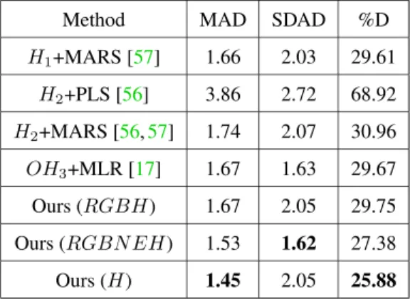
3.3 Comparison of biomass estimation metrics to other methods and with different input channels (H ≡ DEM,Red,Green,Blue,Near-infrared, and redEdge) . . . 30

4.1 Results of our D2S models compared to SegNet as a baseline on the validation set. . . 35

5.1 Results on CARPK and PUCPR+ datasets . . . 46

5.2 Results on the WorldExpo test set . . . 48

5.3 Results on the VGG-Cells testset . . . 48

6.1 Statistics of the datasets used for evaluation . . . 57

6.2 GSP-GAP comparison on CARPK dataset . . . 59

6.3 Results on CARPK dataset . . . 60

6.4 GSP-GAP comparison on ShanghaiTech-A dataset . . . 60

6.5 GSP-GAP comparison on ShanghaiTech-B dataset . . . 62

6.6 Results on ShanghaiTech dataset . . . 62

6.7 GSP-GAP comparison on COWC dataset . . . 63

6.8 Results on COWC dataset . . . 63

L

IST OF

F

IGURES

2.1 Block diagram of our approach. . . 9 2.2 Sample images from the training set of CVPPP-2017 dataset [5,16,68,88]. Representative images are

taken and scaled from 4 training directoriesA1,A2,A3, andA4, respectively. . . 9 2.3 SegNet architecture [14] used for leaf segmentation. Each of the convolution and deconvolution layers is

followed by batch normalization (BN) [48] and rectified linear unit (ReLU). All the pooling operations are2×2max-pooling with stride of 2. Similarly, the unpooling operations are2×2max-unpooling using the pooled indices taken from their corresponding max-pooling operations in the front-end of the network. . . 10 2.4 Sample images with corresponding binary segmentations: original RGB images (top row), corresponding

ground truth segmentations (middle row), and our segmentation results generated by SegNet (bottom row). 11 2.5 Counting architecture used for estimating the number of leaves from SRGB (Segmentation + RGB)

channels. Each of the convolution blocks is a combination of convolution, local reponse normaliza-tion [55], and rectified linear unit (ReLU). All the pooling operations are2×2max-pooling with stride of 2. . . 12 2.6 Augmentation samples for training the counting network. . . 14 3.1 Eleven leaves in an image from the standard leaf counting dataset [16] (left) and eleven wheat plants in

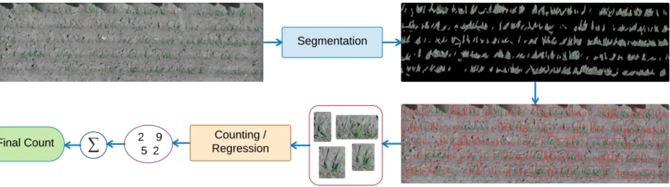
an outdoor image used for emergence counting in this chapter. Counting plants from the right image is more challenging to due to variable number of leaves per plant and occlusion. . . 20 3.2 Workflow for emergence counting: 1) loosely segment the plant regions from RGB plot images with

the segmentation module, 2) extract small patches containing plants via connected component analysis, 3) use counting module for individual counts on each patch, 4) sum all the patches to get the overall emergence count for a single plot. . . 22 3.3 Manual ground-truth generated for relaxed segmentation of plants showing manually drawn contours

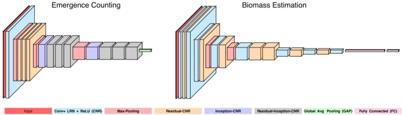
around plant regions (red). Later, contours are filled with simple morphological hole-filling to create the binary segmentation mask. . . 23 3.4 Emergence and biomass estimation architectures. We use7×7receptive fields in the initial CNR

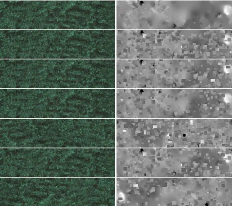
block with unit stride. The number of filters after each max-pooling operation is doubled, except the first one for emergence counting.residual-CNR is a simplified version of the residual block described in [44], where we keep the number of receptive fields constant inside the block. We use a simplified “Inception" module [104], where the number of input and output receptive fields are the same. Inside our Inception block, we employ half of the size of filters for3×3convolution, a quarter of the input size for the equivalent5×5convolution, and half of the rest for pooling and unit convolution each. For the emergence network, to visualize the representations learned by our model, we use global average pooling (GAP) [62]. . . 24 3.5 Sample RGB plot images (left) with corresponding DEMs (right) showing wheat plants from emergence

as individual plants (top) to full crop canopy (middle) and during the reproductive stage (bottom). DEM values (height) converted to grayscale for visualization. . . 25 3.6 Sample RGB plot images (left) with corresponding DEMs (right) showing the original image (top row)

and images generated by ourRMRSdata augmentation procedure (other rows). DEM values (height) converted to grayscale for visualization. . . 26 3.7 Normalized summation of the elevation for the samples augmented from a single image. The first point

represents the elevation of the original sample and the rest(499)are the augmented ones. The range of normalized elevation is in the range[∼0.99,1.0]indicating that the total elevation for all the samples are similar to the original. . . 27 3.8 Sample RGB images (left), their CAM [122] visualizations (middle), and superimposed images (right).

Note that, RGB images are padded by black to maintain a constant size of224×224. Red and blue indicate the most and the least significant regions responsible for emergence counting. As you can see, the plant bases are detected as the most salient regions (red) which the experts also use for counting followed by the leaves (yellow). . . 29

4.1 D2S models with ResNet50 (top) and VGG16-BN (bottom) backbones. Because of the differences in the shape of the final output layer, the placement of the rearrangement or depth-to-space block is different for these models. The last one or two convolution operations incur a negligible computational cost due to the small number of channels (2). . . 33 4.2 (Left to Right) Sample image; Segmentation maps generated by ResNet50-D2S, VGG16-BN-D2S, and

Segnet models, respectively. . . 35 5.1 (Left) Sample images from the CARPK [46] dataset; Superimposed CAM for the VGG-GAP model

trained with only smooth L1 loss (Middle), and joint smooth L1 loss and our proposed heatmap loss (Right). Training with smooth L1 loss exhibits probable false detections for parts of the train and painted wall (red boxes) and probable missed instances for black-colored cars and regions under shadow (green boxes). Without using additional annotations, our heatmap loss fixes both of these problems with more compact activations. Best viewed in digital format. . . 37 5.2 Sample cropped images (top) paired with the corresponding ground-truth Gaussian activation maps

(GAM) generated from the dot annotations (bottom) for CARPK [46] (left), VGG-Cells [60] (middle), and WorldExpo [117] (right) datasets. . . 42 5.3 We take the first 4 sets of convolution and nonlinear activation layers from VGG16 [98] network, replace

ReLU [55] with its parametric version [42], and attach with it a global average pooling (GAP) [62] and a linear layer. Our heatmap loss is the mean absolute difference between CAM low-resolution gaussian activation map (GAM). The double arrow (dark red) indicates that the heatmap loss is backpropagated only through the convolution layers. . . 43 5.4 Superimposed CAM realizations on the images from CARPK (top) and PUCPR+ (bottom) generated by

conventional training (left) and enhanced training with the additional heatmap loss(right). Best viewed in digital format. . . 45 5.5 Superimposed CAM heatmaps on the sample images for the VGG-GAP baseline (top) and

VGG-GAP-HR (bottom) models. Best viewed in digital format. . . 47 5.6 Superimposed CAM heatmaps on the sample images from VGG-Cells dataset from the VGG-GAP

baseline (left) and VGG-GAP-HR (right) models. Best viewed in digital format. . . 49 6.1 (Left) Sample image with multiple cropping shown using bounding boxes with different colors. (Right)

Activations of the first 48 elements sorted in descending order incurred by these cropped samples after GSP operation shown using the corresponding colors of the bounding boxes in the left. For consistency, sorting indices of the full-resolution input are used to sort others. The plot of the values demonstrates the fact of learning a linear mapping of the object counts by our GSP-CNN model regardless of input shape. . . 53 6.2 Sample image for car counting [46] along with superimposed activation heatmaps for different one-look

regression models: (top-left) original image, (top-right) the baseline GAP model, (bottom-left) our GSP model trained with full-resolution images, and (bottom-right) GSP trained with 224×224 randomly cropped patches. . . 55 6.3 Activation maps for CARPK generated by the GAP-Full (left), GSP-224 (middle), and GAP-224(right)

models. Activations are more uniformly distributed and more concentrated inside object regions for the GSP-224 model. . . 59 6.4 (Left) Saliency maps generated by the best GSP models on ShanghaiTech-A (top) and -B (bottom)

datasets. (Right) Same for the best GAP models. GSP and GAP models exhibit similar activations, except GSP models are free fromrandom nullificationeffect due to single inference on full image. . . 61 6.5 Superimposed activation maps for GSP-64 (left) and GSP-224 (right) on the cropped image of COWC

dataset. Activations are better localized the GSP-64 model. . . 63 6.6 Cropped sample images from Wheat-Spike dataset (left) with superimposed CAM generated by

S

TATEMENT OF

A

UTHORSHIP

The chapters in this thesis contains the work published or submitted in the conferences, workshops, and journals listed below:

• Chapter2: Leaf counting with deep convolutional and deconvolutional networks

S. Aichand I. Stavness.Proceedings of the 2017 IEEE International Conference on Computer Vision Workshops (ICCVW), Venice, Italy.

This paper ranked2nd_{place in the Leaf Counting Competition (LCC2017), and got best poster award at the} CVPPP workshop.

• Chapter3: Deepwheat: Estimating phenotypic traits from crop images with deep learning

S. Aich, A. Josuttes, I. Ovsyannikov, K. Strueby, I. Ahmed, H. S. Duddu, C. Pozniak, S. Shirtliffe, and I. Stavness. 2018 IEEE Winter Conference on Applications of Computer Vision (WACV).

• Chapter4: Semantic Binary Segmentation using Convolutional Networks without Decoders

S. Aich, W. van der Kamp, and I. Stavness.2018 IEEE Conference on Computer Vision and Pattern Recognition Workshops (CVPRW).

This paper ranked5th_{place in the Road Segmentation Challenge at the DeepGlobe workshop.}

• Chapter5: Preventing False Localization in One-Look Object Counting Models

S. Aichand I. Stavness.Under review in Pattern Recognition Letters (Elsevier). The preliminary version of this work is also available in arxiv.org as follows:

Improving Object Counting with Heatmap Regulation. S. Aich and I. Stavness.arXiv:1803.05494.

• Chapter6: Object Counting with Small Datasets of Large Images

S. Aichand I. Stavness.Under review in 2019 IEEE Conference on Computer Vision and Pattern Recognition Workshops.

All the computational aspects reported in these papers, from data augmentation to architectural design, implemen-tation, and training are accomplished by me under the supervision of Dr. Ian Stavness. Rest of the authors mostly contributed to the collection of data and preparation of manuscripts.

1. INTRODUCTION

1.1

Problem Definition

Counting object instances from images and videos is a common and practical computer vision task found in a range of applications, such as counting vehicles from aerial images [46,70,76], crowd counting for surveillance [22,60,

87,100,117], biological cell counting for medical diagnosis [60,111,112], plant counting for image based plant phenotyping [37,74,82,84,89,106], and so on. From a broader, more theoretical perspective, object counting can be categorized as a sub-domain of object detection which is a subspace of instance-level segmentation. In this regard, solving the problem of instance segmentation is sufficient (not necessary) to provide solutions for both object detection and counting. However, instance segmentation [41] and object detection [81,83] pipelines demand annotation images with much higher specificity as compared to mere object counting frameworks. Obtaining large-scale annotated datasets with fine granularity is a prohibitively time-consuming process. Thus, specialized and computationally efficient counting approaches that exhibit similar performance with weaker image labels (i.e., dot annotations as compared to bounding boxes or pixel-level masks) are worth pursuing for real-time autonomous vision systems where an object count alone is needed.

In this thesis, we investigate the idea of deep learning, more specificically convolutional neural networks (ConvNets), for object counting from visual data acquired from various sources. In the realm of deep learning, two different kinds of approaches have gained popularity as the possible solution for counting problems:

• The older one, density map estimation followed by additional post-processing, has its root in the conventional feature extraction with classification or regression based frameworks [12,33,60]. With the recent emergence of deep learning, the old-fashioned, constant-dimensional feature extraction based density estimators have been replaced by convolutional networks [13,26,77,91,111,112]. Nonetheless, post-processing steps are needed to retrieve the final count resulting in a multi-stage process. Moreover, these kind of density estimation networks belong to the family of encoder-decoder type architectures, incurring additional computation-cost due to the extra decoder sub-network compared to simple encoder-only type models.

• The later option that evolved recently, one-look regression models [46,70], are the encoder-only convolutional networks. They are very similar to the classification architectures [44,55,98] with the only difference that in regression models, there are either a single output unit responsible for generating the scalar count [46] or the number of output units is a reasonablesupremumof the number of objects in a single image [70]. Regardless of the choice of output layer, these one-look models are both end-to-end and computationally much more efficient compared to their

density estimation based counterparts.

In this thesis, we have chosen the later path of one-look models for exploration due to its comparative efficiency and simplicity in design. We investigate various constraints involved in employing regarding one-look models for object counting in general, such as small datasets and data augmentation, limitations of the standard loss formulations, efficient foreground segmentation, and variable input resolution. In this endeavor, we propose a few useful tricks to adapt the existing one-look models or ConvNet designs to build efficient, general-purpose object counting systems. Although the later chapters follow a progression towards the idea of building a generalized object counting pipeline, these chapters are either published or under submission as standalone manuscripts, and so, can be read independently. Below we provide a brief account of the contributions inscribed in each chapter.

1.2

Contributions

• Chapter2:In the domain of object counting, our journey started through the participation into the CVPPP 2017 Leaf Counting Challenge (LCC), where we obtained reasonable accuracy by training a single, moderately large, VGG-style ConvNet to count leaves from top-down images of rosette plants. Our approach used segmented leaf images from all categories, and was trained from scratch with data augmentation based on simple image processing. Before us, the recent work on the similar dataset used tiny, customized models, one for each category of images. Moreover, the other competitors finetuned very large, pre-trained models on the small-scale competition dataset to achieve state-of-the-art performance. In this regard, we were the first to train a considerably large ConvNet from scratch with few hundred training samples for homogeneous object counting without significant overfitting. The full story of this implementation is depicted in Chapter2.

• Chapter3: The datasets used in Chapter2comprise images acquired in highly controlled environment. At this point, our curiosity drove us to explore similar techniques developed in the previous chapter for images captured in uncontrolled, outdoor environments. Henceforth, we conducted similar experiments for two plant datasets. The first one is for counting the number of early-season wheat plants in sufficiently high-resolution images captured with a GoPro camera. The second dataset is for estimating aboveground biomass from very low-resolution drone images and their corresponding digital elevation maps. As expected, we found it harder to make the simple feedforward ConvNets converge on these more difficult datasets. Therefore, we had to equip our ConvNets with more recent techniques used in advanced architectures, like Inception and ResNet, for reasonable performance. Apart from the architectural engineering, our second contribution was to devise a simple superpixel based data augmentation strategy under the assumption of similarity of minute sub-regions with similar spatial statistics, which we call randomize minimal region swapping (RMRS). In fact, RMRS made it possible for us to train the ConvNets with only 48 low-resolution, drone-plot images. Therefore, training of ConvNets with both high- and low-resolution outdoor plant images and the RMRS data augmentation strategy constitute the body of Chapter3.

ConvNet models for robustness. In Chapters2and3, we employed SegNet [14] for semantic segmentation that has a computation-costly decoder following the encoder sub-network. In general, semantic segmentation architectures are configured in this encoder-decoder style with the assumption that the decoder uses necessary features extracted by the encoder to produce the desired output. This assumption is both highly intuitive from the perspective of convolution and provides good results. However, this rule can be violated if ConvNets are regarded as merely sparsely-connected graphs. In that case, it might be possible to generate the segmentation map directly at the backend of the encoder with depth-to-space reordering of the spatial elements incurring no computational cost. Chapter4exhibits quite satisfactory results for simpler problems like binary segmentation with this perfectly reasonable, but somewhat iconoclastic view. The possible significance of our initial result lies into the heart of overfitting problem for smaller datasets. The lack of additional weight layers after the encoder (or, may be only one for smoothing) would make it straightforward to finetune pretrained encoders directly without the need for highly customized and tricky training procedures for lower cardinality problems like leaf segmentation used in Chapter2.

• Chapter5: In the previous chapters, we mostly focused on training one-look ConvNets, similar to the standard image classification architectures, to regress the scalar count from the images. Although weak spatial information are available to almost all the counting datasets (e.g. a dot annotation on the center of each object in the image), the loss formulation for those models only takes the difference between the absolute counts into account. The possible ramification of this overly simple, scalar measure is the complete lack of minimal guidance to the model about the properties of the target objects to search for. Consequently, simple one-look models tend to fail on seemingly ambiguous cases, i.e. harder instances as well as object-like sub-regions in the background. To alleviate this problem, in Chapter5, we devise a weak or approximate loss based on Class Activation Maps (CAM), a well-known visualization trick, without using additional annotations, and use it alongside the rudimentary L1 loss, that eventually improves both quantitative and qualitative performance of the one-look models.

• Chapter6:This chapter addresses a common challenge in many object counting datasets. These datasets, esp. aerial image databases, often comprise small number of high-resolution, variable-shaped training samples. While training the counting models, we mostly care about the number of instances, not the number of images and so, the receptive field just needs to cover the resolution of the largest possible instance in the dataset. Therefore, it is possible to train with randomly cropped patches of the high-resolution images. However, on inference, if we aggregate the counts by tiling the patches, it causes severe overestimate and underestimate because many object instances will be cut-off at the edge of the patches. However, in many cases, the opposite nature of these two errors helps nullifying each other, resulting in a false impression of low error over the full-resolution image. We coined this event “random nullification" due to its uncontrolled nature considering the weaker ground truth annotation available. Through comprehensive experimentation, we show that the unnormalized GAP (which we call Global Sum Pooling) can avoid this error in a very simple and elegant manner.

1.3

Terminologies

Some of the terminologies and mathematical forms used in the later chapters are listed below:

• Ablation study:In medical science, “ablation” refers to the removal of some body tissues (esp. problematic ones) by surgery. However, in deep learning literature, an ablation study is the comparative performance analysis after removing various components of the models. This kind of analysis is used to understand the effect of different critical components in the proposed architectures.

• Lqloss:This is also known as theMinkowskiloss [18]. The formulation is given by the following equation:

Lq(y, t) =

Z Z

|y(x)−t|q_{p(x, t)dxdt (1.1)} where,x,y,tare input, output, and target variables, respectively. In the machine learning literature,L1 andL2 instantiations of this general loss formulation are used in practice.

2. L

EAF

C

OUNTING WITH

D

EEP

C

ONVOLUTIONAL AND

D

ECONVOLUTIONAL

N

ETWORKS

In this chapter, we investigate the problem of counting rosette leaves from an RGB image, an important task in plant phenotyping. We propose a data-driven approach for this task generalized over different plant species and imaging setups. To accomplish this task, we use state-of-the-art deep learning architectures: a deconvolutional network for initial segmentation and a convolutional network for leaf counting. Evaluation is performed on the leaf counting challenge dataset at CVPPP-2017. Despite the small number of training samples in this dataset, as compared to typical deep learning image sets, we obtain satisfactory performance on segmenting leaves from the background as a whole and counting the number of leaves using simple data augmentation strategies. Comparative analysis is provided against methods evaluated on the previous competition datasets. Our framework achieves mean and standard deviation of absolute count difference of1.62and2.30averaged over all five test datasets.

2.1

Introduction

Traditional plant phenotyping, which involves manual measurement of plant traits, is a slow, tedious and expensive task. In most cases, manual measurement techniques use sparse random sampling followed by the projection of those random measurements over the whole population which might incorporate measurement bias. Further, plant phenotyping has been identified as the current bottleneck in modern plant breeding and research programs [35].

Therefore, interest in image-based phenotyping techniques have expanded rapidly over the past 5 years. Automation of the estimation of these visual traits up to a satisfactory level of accuracy using suitable computer vision techniques can boost production speed and reduce costs since fewer field technicians would be required for manual measurement each year.

In this chapter, we work on estimating the number of leaves on a plant at the rosette stage, which is an indicator of plant health [68]. Our main objective is not only to develop a robust computer vision model, but also to generalize it so that the plant breeders can use this framework regardless of the plant species they are working on and of the quality of the image data they have acquired. Like one of the previous works [37], we also pose this problem as a nonlinear regression problem, where given the images, our framework approximates the count directly without segmenting individual leaf instances. This regression hypothesis is useful for a couple of reasons. First, although this nonlinear regression problem appears to be very high dimensional, it is usually more efficient than counting by identifying the individual leaf instances. Second, from the perspective of supervised machine learning, collecting ground-truth leaf counts is much simpler than

generating ground-truth segmented regions for each leaf in the color images. In section2.4of this chapter, we show that the performance of the systems developed under the regression hypothesis is comparable to the state-of-the-art counting by instance segmentation approaches. However, unlike [37], we develop each of the components of our complete model in such a way that it can directly learn from the data without the need for manual heuristics or explicit knowledge on the plant species or other environmental factors. According to the state-of-the-art computer vision and machine learning literature, the best way to develop a generalized model without such prior knowledge is to use deep learning and therefore we adopt this paradigm in our work.

Similar to [106], we train a deep convolutional neural network to count leaves by regression. However, the focus of our present work is to develop a single network that can generalize across different rosette datasets, rather than separate networks each built and tuned to maximize performance on an individual dataset. We also develop a deep convolutional-deconvolutional neural network for automatic whole plant segmentation and explore the effect of using a binary segmentation mask as an additional input channel to the leaf counting network in order to improve generalized performance. We evaluate our method as part of the Leaf Counting Challenge 2017 (LCC-2017) and report performance across the five subsets of the competition dataset. Through this work, we hope to inaugurate the research and development of a useful and generalized system for plant breeders to study leaf development in individual plants and eventually to study crop emergence in the field.

2.2

Related Work

We classify the recent literature performing leaf counting either directly or via instance segmentation into three categories, i.e. Leaf Segmentation Challenge in CVPPP-2014 (LSC-2014), Leaf Counting Challenge in CVPPP-2015 (LCC-2015), and others. Below we provide a brief account of the methods under each of these categories.

LSC-2014:In total, 4 methods evolve from this competition [89]. Although the training dataset for the competition included individual leaf instances indicated by different colors as the ground-truth, none of the 4 approaches use that ground truth to solve the instance segmentation problem. From that standpoint, they are all are eligible for the LCC-2017 competition also. The winner of this competition is IPK [74,89]. This method utilizes3Dhistogram of the Lab color space of the training images to model both plant regions and background and test pixels are inferred non-parametrically using direct interpolation on the training data. Then, leaf centers are extracted using mathematical morphology of the distance map of the segmented foreground. These centers along with the foreground segmentation are processed by heuristics-based graph algorithms to generate final instance segmentation map. Next, comes the unsupervised Nottingham approach [89], which segments the foreground using seeded region growing [7] over the superpixels [6] extracted from the Lab color map. For the subsets of the dataset containing non-overlapping images, empirical thresholds are used instead of the superpixel means as the initial seed. Like IPK [74], they compute the distance map over the foreground pixels. Then, superpixels with centroids nearest to the local maxima in the distance map are chosen as the initial seeds with the assumption that they represent leaf centers the best for watershed based instance segmentation [107]. The MSU approach is adopted from the literature on multiple leaf alignment and tracking [113–115] and primarily based

on template matching based on Chamfer Matching algorithm [15]. The authors use empirical threshold on the “a" plane of the Lab image to select foreground candidates on which template matching is performed. The main drawbacks of this approach are manual selection of both the threshold and the templates and exhaustive template matching with a large number of templates, i.e.1080templates for2subsets and1920for another. The last method submitted in LSC-2014 is Wageningen [89]. To segment the plant regions, the authors of this approach train a simple artificial neural network comprising one hidden layer of10units with six pixel-based features, i.e. red (R), green (G), blue (B), excessive green (2G−R−B), and variance and gradient magnitude of filtered green pixel values, and then post-process the network output using morphological operations with heuristically chosen parameters. After that, watershed transform [39] followed by empirical threshold based merging is performed to produce the instance segmentation result. A limitation of this method is the use of simple pixel features for foreground segmentation without using any contextual information in depth, resulting in the heavy usage of morphology to fine-tune the network output afterward.

LCC-2015:Only the winning method of LCC-2015 competition, General Leaf Counting (GLC) [37], is published in CVPPP-2015. To the best of our knowledge, this is the first approach posing the leaf counting problem as a nonlinear regression problem. The authors transform the original RGB image into a log-polar image [11] prior to further processing it to exploit the radial structure of the plants. Next, from the log-polar image, they extract patches based on the ground-truth foreground-background ratio in a sliding window fashion. These patch features are further vectorized with K-means [18] and triangle encoding [25]. Lastly, max-pooling over the patch features is performed to form the final feature vector for each image and a support vector regression network [28,37] is trained for the prediction task. A limitation of this system is that the authors use ground-truth plant segmentations in both training and testing phases of the counting module. While approximate plant segmentations could be generated by other methods [67], the study used perfect segmentations and therefore it is not clear how robust their counting module is to noisy or imperfect segmentations that are typical of automatic segmentation procedures.

Others:All the methods proposed since LCC-2015, addressing either the direct counting problem or counting by instance segmentation are found to be based on deep learning, which is not surprising given the resurgence of this subfield of machine learning in recent years. In the recurrent instance segmentation (RIS) approach [84], the authors harness the power of sequential input processing of recurrent neural networks (RNN) [40] with the convolutional version of LSTM cells [45] to segment out one leaf instance at a time. Unlike the use of LSTM and RNN in natural language processing, the idea is to use convolutional LSTM instead of the original formulation to facilitate the training of the network by mitigating the computational complexity of fully connected layers as well as exploiting the semi-global statistical properties of images. To deal with the problem of possible ordering of individual instances in the image, the authors formulate the loss function based on the relaxed version of intersection over union (IoU) [53] and cross-entropy. The work done by Ren and Zemel [82] also use RNN similar to RIS [84]. However, their approach is primarily focused on extracting small patches each time to segment one instance using a similar idea of recurrent attention model [69] and then processing that small patch with LSTM [45] and a deconvolutional network [72] like architecture to segment a single instance. At the time of this writing, this work demonstrates the state-of-the-art performance for instance segmentation. Both this work and RIS use instance-level ground truth to train their networks and are therefore not

Segmentation

Result Counting by

Regression

Figure 2.1:Block diagram of our approach.

directly comparable against ours. Nonetheless, we list their performance results in theExperimentssection. Finally, the deep plant phenomics (DPP) approach [106] proposes a method addressing the problem of counting directly without both plant segmentation and instance segmentation. The authors customize their architectures as well as input dimensions to achieve state-of-the-art accuracy on different subsets of the LCC-2015 dataset. However, it is not known if the approach would generalize and if a single DPP network would provide consistent results across all datasets. Moreover, their training strategy relies on certain assumptions based on the nature of the images available in the LCC-2015 dataset; therefore, it is not clear how this approach would perform on the new types of images in the LCC-2017 competition. We will provide a detailed discussion about these issues while comparing our framework to DPP in section2.4.

2.3

Our Approach

The approach presented in this section is developed to participate in the LCC competition [5] at CVPPP 2017. The high-level design of our framework follows a traditional computer vision workflow where the segmentation module is followed by the counting module (Figure 2.1). Within each module, we incorporate task-specific convolutional architectures, which are trained without explicit knowledge of the plant species to develop a generalized framework able to learn only from the data. The architectures used for segmentation and counting are trained separately, but not independently since the binary mask generated by the segmentation model is used to train the counting model in conjunction with the RGB channels. In the following two subsections, we will describe the architectures along with the rationale behind their design. Training methodologies and data augmentation strategies for these models are described in the experiments section.

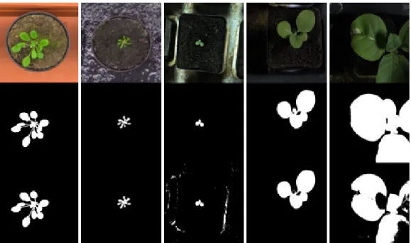
Figure 2.2:Sample images from the training set of CVPPP-2017 dataset [5,16,68,88]. Representative images are taken and scaled from 4 training directoriesA1,A2,A3, andA4, respectively.

Input(RGB) Convolution + BN + ReLU Max-Pooling Deconvolution + BN + ReLU Max-Unpooling Output(Probability) RG BImage Probabilit y Output

Figure 2.3:SegNet architecture [14] used for leaf segmentation. Each of the convolution and deconvolution layers is followed by batch normalization (BN) [48] and rectified linear unit (ReLU). All the pooling operations are2×2max-pooling with stride of 2. Similarly, the unpooling operations are2×2max-unpooling using the pooled indices taken from their corresponding max-pooling operations in the front-end of the network.

2.3.1

Segmentation

The segmentation problem we address is that of differentiating the plant or foreground pixels, from the background. This kind of problem is also known as semantic segmentation where the semantics of the objects are utilized to accomplish the task. In recent years, many papers [23,65,120] have been published addressing the solution for semantic segmentation from RGB images. Some of these architectures belong to the class of neural networks called deconvolutional networks[14,72]. The main idea behind this kind of network is to construct a compact and informative set of feature maps or vectors from a set of input images, and then generate class-probability maps from the feature maps. Like other convolutional networks, construction of the feature set from the input data is done by a convolutional network comprising multiple layers of convolution, pooling, and normalization operations. This convolutional sub-network is followed by a deconvolutional sub-sub-network consisting of convolution-transpose, unpooling, and normalization operations to generate the desired probability maps. From the standpoint of semantic segmenatation, both height and width of the input and the output are the same. Hence, the deconvolutional part of the network is designed as a mirrored version of the convolutional part, except the input and the output layers, irrespective of the complexity of the problem and the dimensionality of the class-space.

Usually the design of a deconvolutional network contains fully connected (FC) layers in the middle to generate the feature vector from the pooled feature maps [72]. The FC layers are used to extract features in the global context for segmentation, and are therefore important if global context is necessary for the segmentation task. However, we propose that features in the semi-global context should be sufficient to segment the leaf regions from the background in color images, and therefore the FC layers could be omitted for our application. An advantage of eliminating the FC layers is that it considerably reduces the number of trainable parameters without sacrificing performance. For these reasons, we adopt the SegNet architecture [14], which omits FC layers and has shown promising results on SUN RGB-D [101] dataset comprising complicated indoor scenes and CamVid [20] video dataset of road scenes. The removal of FC layers in SegNet results in about 90% reduction of the number of trainable parameters as well as computational complexity. Figure2.3depicts the segmentation network we employ. The front-end convolutional sub-structure of the network is the VGG architecture [98] with batch normalization followed by each convolutional layer. In the convolutional front-end of

Figure 2.4:Sample images with corresponding binary segmentations: original RGB images (top row), corre-sponding ground truth segmentations (middle row), and our segmentation results generated by SegNet (bottom row).

SegNet, there are five2×2pooling operations with zero overlapping following multiple convolution and rectification layers each time. Hence, the convolved feature maps are compressed32times before starting the decompression via the deconvolutional back-end. We hypothesize that such level of compression or semi-global consideration is qualitatively sufficient to solve a comparatively easier problem of whole plant segmentation (Figure2.2) as compared to other domains of semantic segmentation.

2.3.2

Counting

As shown in Figure2.1, we use both the RGB image and the corresponding binary segmentation image to estimate the number of leaves after the segmentation is done. The rationale behind providing the counting module with the segmentation mask and the original RGB image instead of providing either the segmented region in the RGB image or the binary mask alone will be evident from Figure2.4. Although the segmentation results generated by SegNet are sufficiently accurate for the counting phase for many images in the dataset, our network generates spurious segmentations for few of them. The poorly segmented images generally have lower average intensities and regions of leaves where the color and texture properties are washed out or blurred. We expect our network to do more or less accurate segmentation for these images by using semi-global contextual information, but we believe it fails due to the low number of available samples of that kind in the training dataset both in terms of absolute count and ratio of the samples of this particular kind to other kinds. The problem of this data scarcity is specific to the data-hungry approaches like deep learning, which requires a substantial number of training instances of a particular prototype to generate an accurate input-output mapping for that specific type.

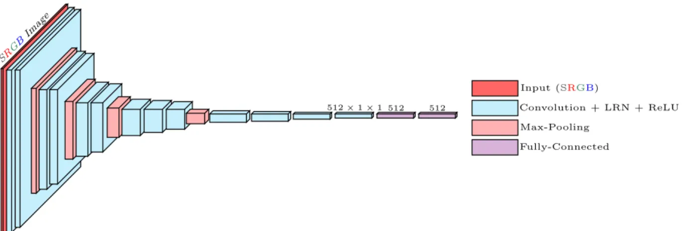
512×1×1 512 512 Input (SRGB) Convolution + LRN + ReLU Max-Pooling Fully-Connected SRG BImage

Figure 2.5:Counting architecture used for estimating the number of leaves from SRGB (Segmentation + RGB) channels. Each of the convolution blocks is a combination of convolution, local reponse normalization [55], and rectified linear unit (ReLU). All the pooling operations are2×2max-pooling with stride of 2.

recover the missed plant regions as well as reject the false detections from original image with the help of segmentation mask for counting. We call this four channel input as the SRGB (Segmentation + RGB) image. We also expect that providing the segmentation channel as input to the leaf counting network will help to suppress bias from features in the background of the training images, such as the soil, moss, pot/tray color, which will vary between datasets.

The design of our leaf counting by regression network takes inspiration from the VGG architecture [98], which reinforces the idea of deeper architectures with a long list of convolutional and rectification layers stacked one after another with several pooling layers in between and then the classification layer follows a couple of fully connected layers. Usually, this kind of convolutional networks use suitable amount of padding to maintain fixed height and width of the feature maps. Padding the input maps serves well when the network is trained with large-scale datasets containing samples in the order of millions. However, in our case, we have a small dataset of several hundred images to train, which is very difficult to augment beyond several thousand images. Hence, to retain the power of deeper architecture and to train the parameters without significant overfitting at the same time, we reduce the number of parameters effectively by using convolution without padding throughout the network. Moreover, we choose the filter size of the convolutional layers in such a way that before proceeding through the fully connected layers, the feature map turns into a vector. Thus, with zero padding and careful choice of filter size, we are able to reduce the number of parameters from49M to30M. Implementation details for both segmentation and regression networks are provided in the following section.

2.4

Experiments

In this section, we provide a detailed account of our experimental setup. First, we describe the dataset used for evaluation. Next, the training strategies for both networks are specified. Finally, the performance of our framework is analyzed and compared against state-of-the-art literature from both quantitative and qualitative standpoints.

2.4.1

Dataset

The dataset we use to evaluate our framework is provided to the teams registered for the Leaf Counting Challenge (LCC-2017). The objective of this challenge is to come up with the solutions able to count the number of leaves from plant images directly via learning algorithms without detecting individual leaf instances. All the RGB images in the dataset belong to either Tobacco or Arabidopsis plants. For the LCC competition, each RGB image is accompanied by a binary segmentation mask with1and0indicating plant and background pixels, respectively, and a center binary image with leaves centers denoted by single pixels.

The training dataset is organized into4directories, namelyA1,A2,A3, andA4. DirectoriesA1andA2contain Arabidopsis images taken from growth chamber experiments with larger but different field of views covering many plants and then cropped to a single plant. DirectoryA3enlists the Tobacco images with the field of view chosen to encompass a single plant.A4is a subset of another public Arabidopsis dataset [16] collected using a time-lapse camera. In total, there are27Tobacco images inA3, and783Arabidopsis images in the rest of the directories. The organizers denote these directories along with the images as “SPLIT" images since they are split into separate folders according to the origin. In addition, all these directories contain CSV files including ground truth leaf counts under the same nomenclature.

The “SPLIT" directory structure for the testing set is the same as training, except that it includes an extra directory denoted byA5, enlisting images from different sources of origin altogether with the objective to emulate a leaf counting task in the wild. Hence, the organizers representA5images under the nomenclature “WILD".

2.4.2

Training and Implementation

SegNet training:Unlike training in the original SegNet paper [14], we trained our model from scratch without using any pretrained weights for initialization. Also in SegNet, the authors used different learning rates for different modules, whereas a fixed learning rate was used for all the layers in our training.

We used an input and output image size of224×224pixels in SegNet, whereas the original image size was approximately500×500and2000×2500. While training deeper networks, the obvious advantage of using smaller input-output size than the original ones is data augmentation up to a considerable amount. We augmented the data and train the network in3stages. First, for each image, we extracted the union of top 20 object proposals [123], flipped top-bottom and left-right, rotated them with an angular step size of 4 degree, cropped the largest square from the center position to avoid dark regions due to rotation, and created a couple of Gaussian blurred version and corresponding sharpened images. In this way, we generated about0.8M augmented samples from810original images and trained the network for 5 epochs with randomly cropped224×224subsamples. Second, we took the proposal images and their flipped versions and generated nearly0.3M subsamples of size224×224deterministically with a fixed stride and train the network for another 8 epochs. Finally, we generated another0.19M samples in a similar manner as in the second step, but this time from the original images instead of the proposals. Then, we fine-tuned the network with these0.19M samples for 37 epochs. In all stages, SGD-momentum was used as the optimizer with initial learning rate, momentum

and weight decay of0.01,0.9, and0.0001, respectively and these parameters were changed later based on the training statistics. Spatial cross-entropy was used as the error criterion. The ratios of foreground to background weights in the cross-entropy calculation for the first stage was2.0and1.2for the later steps. In the test phase, we took dense224×224

samples deterministically with fixed stride from each of the test images and classified each pixel based on the aggregate probability over the samples. We initialized the convolutional weights with Xavier [38] prior to the start of training.

Figure 2.6:Augmentation samples for training the counting network.

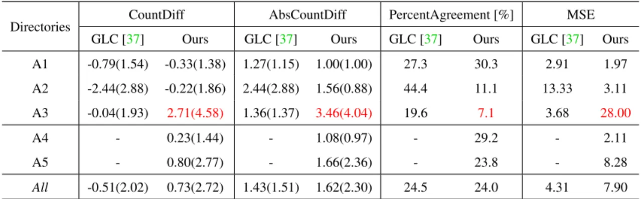
Table 2.1: Head-to-head comparison against LCC-2015 winner. Note thatAllrefers to A1-A3 for GLC and A1-A5 for Ours.

Directories CountDiff AbsCountDiff PercentAgreement [%] MSE GLC [37] Ours GLC [37] Ours GLC [37] Ours GLC [37] Ours A1 -0.79(1.54) -0.33(1.38) 1.27(1.15) 1.00(1.00) 27.3 30.3 2.91 1.97 A2 -2.44(2.88) -0.22(1.86) 2.44(2.88) 1.56(0.88) 44.4 11.1 13.33 3.11 A3 -0.04(1.93) 2.71(4.58) 1.36(1.37) 3.46(4.04) 19.6 7.1 3.68 28.00 A4 - 0.23(1.44) - 1.08(0.97) - 29.2 - 2.11 A5 - 0.80(2.77) - 1.66(2.36) - 23.8 - 8.28 All -0.51(2.02) 0.73(2.72) 1.43(1.51) 1.62(2.30) 24.5 24.0 4.31 7.90

Count network training:Training of the counting network is fairly straightforward compared to SegNet. In this phase, we used all the images as a whole without prior cropping or sampling operation for data augmentation to ensure that the ground truth leaf counts were valid for all augmented images. Also, while designing the network architecture,

Table 2.2:Comparison against state-of-the-art literature. Note thatAllrefers to A1-A3 for previous work and A1-A5 for Ours.

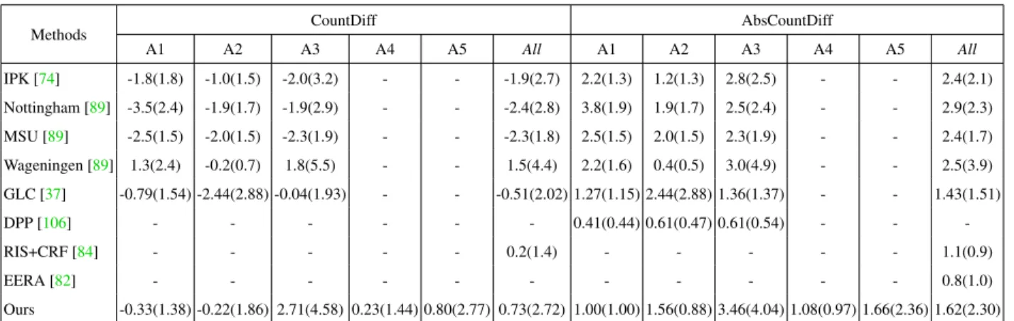
Methods CountDiff AbsCountDiff

A1 A2 A3 A4 A5 All A1 A2 A3 A4 A5 All IPK [74] -1.8(1.8) -1.0(1.5) -2.0(3.2) - - -1.9(2.7) 2.2(1.3) 1.2(1.3) 2.8(2.5) - - 2.4(2.1) Nottingham [89] -3.5(2.4) -1.9(1.7) -1.9(2.9) - - -2.4(2.8) 3.8(1.9) 1.9(1.7) 2.5(2.4) - - 2.9(2.3) MSU [89] -2.5(1.5) -2.0(1.5) -2.3(1.9) - - -2.3(1.8) 2.5(1.5) 2.0(1.5) 2.3(1.9) - - 2.4(1.7) Wageningen [89] 1.3(2.4) -0.2(0.7) 1.8(5.5) - - 1.5(4.4) 2.2(1.6) 0.4(0.5) 3.0(4.9) - - 2.5(3.9) GLC [37] -0.79(1.54) -2.44(2.88) -0.04(1.93) - - -0.51(2.02) 1.27(1.15) 2.44(2.88) 1.36(1.37) - - 1.43(1.51) DPP [106] - - - 0.41(0.44) 0.61(0.47) 0.61(0.54) - - -RIS+CRF [84] - - - 0.2(1.4) - - - 1.1(0.9) EERA [82] - - - 0.8(1.0) Ours -0.33(1.38) -0.22(1.86) 2.71(4.58) 0.23(1.44) 0.80(2.77) 0.73(2.72) 1.00(1.00) 1.56(0.88) 3.46(4.04) 1.08(0.97) 1.66(2.36) 1.62(2.30)

Table 2.3:Possible interpretation of the performance measures.

Measures Possible Interpretation

CountDiff↓ The model is less biased towards overestimate or underestimate. AbsCountDiff↓ Average performance is better.

PercentAgreement↑ Number of accurate predictions is higher.

CountDiff↓, AbsCountDiff↓ Less bias with better performance. Desirable properties of an ideal nonlinear regression model. CountDiff↓, AbsCountDiff↑ High positive and negative errors cancel out. Model behaviour tends to be linear than usual. PercentAgreement↓, AbsCountDiff↓Although many predictions are not exactly accurate, all of the predictions are close to the original;

therefore, model performance is uniform over the samples.

PercentAgreement↑, AbsCountDiff↑Although many predictions are exact, wrong predictions are far from the original;

therefore, model performance is not uniform over the samples.

we experimented with adaptive operations to deal with variable sized images, but they did not seem to work better than resizing the images to a fixed size. Moreover, we had to be cautious in the choice of the size for resizing operation so that for bigger images with resolution like2000×2500, properties of the small leaf regions did not deteriorate much. Considering this fact, we chose the modified image size to be448×448preserving the aspect ratio. Thus, the largest dimension was taken to be448and the smaller one was padded with zeros afterward.

After the resize operation was performed, each of the images was augmented8times using intensity saturation, Gaussian blurring and sharpening, and additive Gaussian noise (Figure2.6). Each image was also flipped top-bottom and left-right and rotated 180◦along with similar augmentations. Thus, we generated36slightly different samples with the same ground truth from each original image, resulting in29160training instances for the regression network.

After the data generation was done, the counting or regression network was trained for 40 epochs using Adam [51] with fixed learning rate and weight decay both set to0.0001. Smooth-L1criterion was used as the loss function instead of simpleL1criterion to prevent gradient explosions as described in [36]. At first, we started training the model with normalized FC layers of size1024. However, based upon the training statistics and to reduce the risk of overfitting, we changed the size of FC layers to512and retrained the model with the already trained convolutional weights. Finally, the

model trained until epoch35was used to generate the prediction for final submission.

Implementation:We used Torch [27] as the deep learning framework for both models. All the convolutional filters of the segmentation network were of size3×3. For regression architecture,9×9convolution was performed until the second max-pooling operation and5×5afterward. We used the convolutional stride of1throughout both networks. All the pooling operations were2×2max-pooling with stride of2. The dimension of all fully connected layers in the regression network was512. Training was performed on a single NVIDIA Quadro P6000 Dell workstation. On this machine, training of SegNet took about6−7days, whereas the regression network was trained within a couple of days.

2.4.3

Evaluation

Evaluation of our complete framework was accomplished in three stages. First, we assessed the segmentation network in terms of the precision and recall (equation2.1) of the plant pixels. Next, we performed a head-to-head comparison against the winner of the previous LCC competition. Finally, we compared our results to the state-of-the-art approaches. We also performed an ablation study by training our counting network with and without the segmentation channel as input, in order to cast some light on the issue regarding the need for foreground segmentation.

Foreground segmentation:Even though the accuracy of binary segmentation is not a criterion for evaluation in the LCC competition [5], we provide precision and recall (equation2.1) of our segmentation model in Table3.1to justify our assumption on the sufficiency of semi-global context for leaf segmentation. It is evident from Table3.1 that the segmentation results generated by SegNet using semi-global information are good enough to be used for the regression network. Performance of the segmentation network is comparatively lower for directoryA3(Table3.1, red text) since there are only27Tobacco images in theA3training set as compared to783Arabidopsis images in the rest of the directories.     

Precision= True Positive True Positive+False Positive Recall= _{True Positive}True Positive_{+False Negative}

(2.1)

Table 2.4:Binary segmentation results.

Directory A1 A2 A3 A4 A5

Precision 0.98 0.94 0.80 0.96 0.92 Recall 0.99 0.99 0.94 0.98 0.97

Comparison against the previous winner: Next, we provide comparisons in both Table2.1and2.2. Table2.2 provides comparisons against all the recent literature, whereas Table2.1provides a head-to-head comparison against the LCC-2015 winner, which is more detailed due to the availability of the performance metrics for [37]. In Table2.1, “CountDiff" refers to the mean and standard deviation (shown in parentheses) of the difference in count averaged over images. “AbsCountDiff" is the absolute of “CountDiff". The term “PercentAgreement" indicates the percentage of exact matches between the actual prediction and ground truth measurement for counts. “MSE" is the abbreviation for

mean-squared error.

From Table2.1, it is evident that we achieve lower CountDiff and AbsCountDiff for directoriesA1andA2. Lower CountDiff means that our model is less biased towards underestimation or overestimation than GLC [37], whereas lower AbsCountDiff can be interpreted as the indicator of better average performance of the system. However, our framework performs poorly on directoryA3(Table2.1, red text). The reason behind the failure is pretty straightforward. Note that, in the training set, there are in total783Arabidopsis images inA1,A2, andA4. On the other hand, there are only

27Tobacco images inA3, which is scarce for the types of deep architectures we are using that contain millions of parameters. Hence, our regression network fails to model the distribution for leaf counting over the Tobacco images. This inadequacy is also reflected in the AbsCountDiff measure for the test directoryA5, which is a mixture of Arabidopsis and Tobacco images altogether.

For directoryA2, although our CountDiff and AbsCountDiff are better than those of GLC, PercentAgreement of GLC is much better than ours. Apparently, it might seem to be a pitfall of our system. However, the combination of lower AbsCountDiff and lower PercentAgreement means that even though the number of exact predictions is low, all the predictions are pretty close to the original and the overall performance of the system is more or less uniform over the test images. On the contrary, comparatively higher values of AbsCountDiff and PercentAgreement, which belong to GLC for directoryA2, refers to the situation where model performance is not uniform over the samples. In other words, predictions may be accurate for easier samples with no leaf overlap or moderate-sized leaves or both, but deteriorate for harder cases with smaller or overlapping leaves. In that sense, our generalized framework is capable of modeling and inferring leaf shapes under deformation and partial occlusion better than GLC given a few hundred images for a particular species. To facilitate this kind of comparative evaluation of our method by the readers, we enlist a set of combinations of the measures along with their possible interpretations in Table2.3. Also, note that our average measurement (directory “All") is over501test images from5directories (A1-A5), whereas the average for GLC is taken over98test images from3directories (A1-A3).

General comparison:Table2.2shows that our method performs well as compared to all the LSC-2014 [74,89] and LCC-2015 [37], except for the failure on directoryA3due to inadequate number of samples. Both RIS+CRF [84] and EERA [82] use instance-level ground truth. Hence, they are eligible for the segmentation competition (LSC), but not the counting competition (LCC). Nonetheless, we put them in the list to demonstrate our comparability to these state-of-the-art methods developed with instance segmentations that are more expensive in terms of training complexity/time and ground truth data requirements. DPP [106] is the only method close to ours in the style of approach, except that they use three shallow regression networks, each one highly customized over a single directory. Moreover, DPP uses random cropping from10%−25%for the purpose of data augmentation while training. This could result in mislabeled images if leaves are cropped out of certain images. The new rosette images in the LCC-2017 dataset include larger rosettes that cover more of the image frame (and extend outside the frame in certain cases, see rightmost image in Figure2.2); therefore it is not clear how DPP would perform on the larger and more varied test images in the new competition dataset.

study by training our regression network using only RGB images as the input without foreground segmentation. We found slower convergence than that of using the segmentation images as input. However, counting results using only RGB images were comparable, which supports the approach proposed by DPP of using a regression network directly on RGB images and that the network learns relevant features directly without a priori segmentation. Nonetheless, we do expect that providing foreground segmentation as an additional input channel helps to push the regression architecture to train on localized features within the plant region in the image. This might help to suppress background features that could limit the generalizability of the counting model if provided images of rosettes grown in different backgrounds, e.g. in different pots, trays, or growth tables. The issue of localization of features in these types of regression networks requires additional attention as future work.

2.5

Conclusion and Future Work

In this chapter, as a participant of the LCC-2017 competition, we provide a complete and generalized data-driven framework for leaf counting from RGB images directly without instance segmentation. We demonstrate that given a moderate amount of data on any species, our architectures are able to learn to estimate the number of leaves without prior knowledge on that particular species or surroundings of the plant. From the perspective of informed search strategies, we do plant segmentation prior to counting with the assumption that the additional foreground segmentation channel guides the regression model to extract necessary features only from the plant region and thus trains the model correctly. However, based upon other recent works and ours, the need for segmentation prior to counting by the deep networks is still an open question. As future work, we plan to investigate this issue in more detail, with the goal of achieving equivalent performance to that of instance segmentation architectures with much simpler and easier to train non-recurrent networks such as reported in the present study.

3. D

EEP

W

HEAT

: E

STIMATING

P

HENOTYPIC

T

RAITS FROM

C

ROP

IMAGES WITH

DEEP

L

EARNING

In this chapter, we investigate estimating emergence and biomass traits from color images and elevation maps of wheat field plots. We employ a state-of-the-art deconvolutional network for segmentation and convolutional architectures, with residual and Inception-like layers, to estimate traits via high dimensional nonlinear regression. Evaluation was performed on two different species of wheat, grown in field plots for an experimental plant breeding study. Our framework achieves satisfactory performance with mean and standard deviation of absolute difference of1.05and1.40

counts for emergence and1.45and2.05for biomass estimation. Our results for counting wheat plants from field images are better than the accuracy reported for the similar, but arguably less difficult, task of counting leaves from indoor images of rosette plants. Our results for biomass estimation, even with a very small dataset, improve upon all previously proposed approaches in the literature.

3.1

Introduction

Measuring the phenotypic traits of crops, which are the differences in plant characteristics caused by the interaction of the plant’s genetics and the environment, is important in plant breeding research as it allows the breeders to select crop varieties with desirable physical characteristics, such as high yield, resistance to stress, and ability to be easily harvested. Traditionally, phenotypic measurements are made manually in the field, which is both labor intensive and potentially inaccurate due to substantial sub-sampling involved. To overcome these drawbacks, image-based automated phenotypic traits estimation is emerging as an important area of applied computer vision research with the goal of capturing more accurate information at a large scale for better crop production.

In many crops, including wheat, emergence (the density of plants within the field) and biomass (the total mass of each plant) are important phenotypes. Emergence is important because a vigorous and uniform crop stand is needed to compete for moisture, nutrients, and sunlight. Plants that emerge late will have a lower yield than the early emerging ones due to the increase in competition for sunlight and essential nutrients [58]. Determining biomass in different crop varieties is important because it is correlated with yield [102] and photosynthetic activity, and is an indicator of overall plant health [30]. These phenotypes are labour intensive and destructive to measure manually: emergence typically requires physically touching plants in the field to determine which leaves belong to which plant, and biomass measurements are made by cutting out plants from the field and measuring their mass. Furthermore, these phenotypes are traditionally measured on only a small sub-sample of the experimental plot area, which can result in sampling error.

Figure 3.1:Eleven leaves in an image from the standard leaf counting dataset [16] (left) and eleven wheat plants in an outdoor image used for emergence counting in this chapter. Counting plants from the right image is more challenging to due to variable number of leaves per plant and occlusion.

The combination of high importance and high measurement difficulty makes these phenotypes good candidates for image-based phenotyping in any crop breeding programs.

Counting plants is related to the well-studied problem of counting leaves from plant images [9,37], but much more challenging. Wheat seeds are planted in close proximity, therefore, the plants grown from these seeds are highly occluded by each other in the image. To illustrate the level of difficulty, Figure3.1shows a sample image from the standard leaf counting dataset [16] and another image from the dataset we are using for wheat emergence counting. Both images have the same label: 11 leaves in the left image, and 11 wheat plants in the right image. In the left image, the number of leaves is unambiguous despite a few small leaves in the center, which is not the case for plant count in the right image. According to the plant science experts who generated the ground truth counts and who have experience counting plants in the field, while counting from the images, they looked at the stems as close to the ground as possible. When a stem seemed unreasonably thick, they presumed that there were more plants behind the visible ones. Plant bases indicated by the yellow arrows in the figure are easy to count. However, in regions denoted by the green arrows, it may look like there is one plant, based on the thickness of the plants, amount of leaves, and age of plants, the count of plants was estimated by the raters as more than one. Hence, both intuition and experience play a role in accurate emergence counting, making it a difficult image analysis task.

In this chapter, we propose completely data-driven frameworks for emergence counting and biomass estimation. We develop generalized architectures for phenotypic traits estimation blending the concepts of learning sparse structure via dense, multiscale representations [103] and residual or shortcut connections [44]. We train our models from scratch to keep our phenotypic estimation tasks independent of the other large-scale machine learning tasks pursued with very large models. For this reason, to efficiently train the data-hungry deep models with a few training samples, we also propose a novel data augmentation strategy based on randomized minimal region swapping of the superpixels in an image, which can be used to augment low to medium resolution images. Also, we examine the quality of learning of the emergence counting architecture qualitatively by visualizing salient regions using the class activation mapping (CAM) [122] approach. We find that the learned network features focus on image regions that are responsible for counting, notably the base of each leaf-cluster, and the dense regions of leaves, according to the plant breeding experts who provided the ground truth counts.