Abstract—In this paper, we present two new procedures for feature selection using a data quality measure. The first procedure is a filter method and the second is a hybrid method that combines the former method with a sequential forward selection (SFS), which is a wrapper method. Three classifiers; LDA, KNN and RPART, are used along with the wrapper method. Comparisons with the RELIEF and the usual SFS method are carried out on twelve well-known Machine Learning datasets. The experimental results show that our filter method outperforms the RELIEF, regarding both the misclassification error rate and the running time. Our hybrid method is faster than the SFS and it gives misclassification error rates quite similar to those given by the SFS.
Index Terms—Feature selection, data preprocessing, supervised classification, data quality.
I. INTRODUCTION
In high dimensional datasets the presence of redundant and irrelevant features deteriorates the performance of data mining algorithms [14]-[15]. Therefore, it is necessary to select a subset of good features to facilitate and improve the data mining process. Traditionally, the feature selection methods have been focused on removing irrelevant features, but in problems of high dimensionality, it is also important to remove redundant features [16].
Several effective feature selection methods had been proposed [1],[3],[5],[8],[10]. However the increment in the size of the dataset in both directions, number of instances and number of features becomes a great challenge for the feature selection algorithms. The handing of high dimensional datasets requires a great amount of both storage and computing time. Thus, the computational costs are severally increased. Finding an optimal subset of feature under these conditions becomes intractable [8]. Algorithms related to feature selection have been shown to be NP-hard.
There are two major types of feature selection methods: Filter methods [5]-[8] and wrapper methods [11],[13],[16]. The filters are pure pre-processing techniques. In these methods, the relevance of each feature is evaluated individually and a Manuscript received March 26, 2008. This work was supported in part by the Office of Naval Research under Grant N00014061098.
Luis Daza is with the Department of Mathematical Sciences, University of Puerto Rico at Mayaguez, Mayaguez, PR 00680, USA (e-mail: luis_dp@ math.uprm.edu).
Edgar Acuña is with the Department of Mathematical Sciences, University of Puerto Rico at Mayaguez, Mayaguez, PR 00680, USA (corresponding author, e-mail: edgar@ math.uprm.edu).
score is given to each of them. The features are ranked by their scores and the ones with a score greater than a threshold are selected. Later, a classifier can be applied using only the selected features. The RELIEF, one of the most used filter methods. was introduced by Kira and Rendell[7] for a two-class problem, and extended later to the multiclass problem by Kononenko[9]. In the RELIEF, the relevance weight of each feature is estimated according to its ability to distinguish instances belonging to different classes. Thus, a good feature must assume similar values for instances in the same class and different values for instances in other classes. The relevance weights are set to be zero for each feature and then are estimated iteratively. In order to do that, an instance is chosen randomly from the training dataset. Then, the RELIEF searches for two closest neighbors to such instance, one in the same class, called the Nearest Hit and the other in the opposite class called the Nearest Miss. The relevance weight of each feature is modified according to the distance of the instance to its Nearest Hit and Nearest Miss. The relevance weights continue to be updated by repeating the above process using a random sample of n instances drawn from the training dataset..
The wrapper feature selection methods need one classifier algorithm in order to select the best features. The quality of a subset of features is determined by the performance of the classifier using such subset. For this reason, the wrappers outperform the filters with respect to the misclassification error. However, the gain in accuracy has a cost in terms of efficiency and generalization since the computational burden increases and also the selection of the best subset depends on the classifier being used. There are three major variations of wrappers, Sequential forward selection (SFS), Sequential Backward selection (SBS) and Sequential Floating Forward (Backward) selection. In this paper, we have considered only the SFS procedure. This algorithm begins considering the best subset of features B, as the empty set, and in each step enters to B the feature that gives the highest increment of the classification accuracy rate. The algorithm stops when the classification accuracy cannot be improved by the remaining features not included yet in B. Other stopping criterion is to check if the size of the subset B exceeds a prefixed number. Recent research on feature selection has been focused to face the challenge of having a large number of instances[10],[13] and handling datasets of high dimensionality[2],[14]. Much of the effort has been dedicated to build hybrid algorithms for feature selection, through combining the advantages of the filters and wrappers methods[12]. However these new methods do not reduce the computational complexity of the existing algorithms.
Luis Daza and Edgar Acuna
The quality of a dataset is determined by internal and external factors. The internal factor reveals if the predictors and the classes has been correctly selected and are well defined. The external factor measures errors introduced in the predictors or in the class assignment, either systematically or artificially. According to Zhu et al [17], the misclassification error rate depends on the quality of the information contained on the training set and on the bias of the induction algorithm used to carry out the classification. This means that improving the data quality of the training set will reduce the misclassification error. The classifier will perform better using a clean training set.
In this paper, we propose two new procedures for feature selection based on a new data quality measure introduced in Daza[4]. The first one is a filter method and it is compared to the RELIEF, the second one is a hybrid method and it is compared to the SFS. This comparison is done in two aspects, the misclassification error rate and the computing running time. The new procedures are applied to twelve datasets using three classifiers: Linear Discriminant Analysis (LDA), a decision tree classifier based on recursive partitioning (RPART) and the k-nn classifier (KNN ). All three classifiers are available in the R system for statistical computation and graphics (http://cran.r-project.org). In the next section, we describe the data quality measure. In section III, the proposed feature selection methods are described in detail. The experimental results are explained in section IV, and the conclusions of the paper are given in the last section.
II. THE DATA QUALITYMEASURE
Daza [4] introduced a measure to evaluate the quality of an instance. This measure takes in account the localization of an instance within its class as well as with respect to the decision boundaries with the other classes. Thus, for the i-th instance of the dataset of size N, its data quality measure is given by
)
,
max(
/
)
(
i i i ii
r
d
d
r
Q
=
−
, i=1,….N, whered
i is thedistance of the i-th instance to the centroid of its class, and
i
r
is the minimum distance of the i-th instance to the centroid of the classes where it does not belong to. Clearly,.
1
1
≤
≤
−
Q
An instance with a Q value near to 1 has a good quality. A noisy instance will have a negative value for the quality measure Q. However, some instances located near to the boundary of two or more classes may also have small positive values for the quality measure. A variant of the measure Q, can be obtained by using the k nearest neighbors of a given instance. In this case,d
i will represent the average distance of the i-th instance to its k-nearest neighbors within its class, andr
iwill be the minimum average distance of the i-th instance to their k nearest neighbors in each of the other classes. More details about the effectiveness of the measure Q can be found in Daza [4].III. THE PROPOSED FEATURE SELECTION METHODS
In this paper, we will introduce two new feature selection procedures. The first one, called Wfeat, is a filter method. The second one, named WfeatSFS, is a hybrid method which combines the Wfeat with the sequential forward selection method (SFS) which is a wrapper method. In the sequel we will describe both methods in detail. We will assume that our training dataset has p features and N instances.
The Wfeat method
In this filter selection method, we evaluate the relevance of each feature according to its capability to reduce the complexity of the decision boundary. The procedure is as follows:
1. For each of the Fj (j=1,..p) features, an univariate quality measure Q(Fj) is computed for each instance of the training dataset.
2. For each feature, the average of the quality measure of the N instances is computed. That is,
N
F
Q
F
Q
N
i
j i j
∑
==
1)
(
)
(
.
3. Each feature has a corresponding relevance weight given by
)
1
)
(
exp(
)
(
F
j=
Q
F
j−
W
4. The p features are ranked in decreasing order according to its relevance weight.
The next step, it will be to decide on the number of features to be selected. An alternative it could be to retain a given percentage, say 60%, of the original instances. Another way is to plot the relevance weight of the features and to choose as the relevant features those with relevance weights appearing above the highest jump in the plot.
The computation of the quality measure Q for each feature is done in linear time in both the number of instances and the number of features. On the other hand, the steps 2 and 3 are done in N steps. Finally, the step 4 of the algorithm has complexity of order
p
log
p
. Hence, the asymptotic complexity of the Wfeat algorithm isO
(
N
×
p
)
. Therefore, this method is efficient in terms of the computation time and in the next section we will show experiments where Wfeat gives on average better misclassification error rates than the RELIEF, perhaps the most well-known filter method. The disadvantage of Wfeat is the same of the most filter methods, it fails to identify redundant features. Next, we will present a second algorithm that tries to overcome this problem and eliminates the redundant features, keeping only the relevant ones.The WfeatSFS method
method. Hence, a classifier L needs to be used. The algorithm is as follows:
1. First, the Wfeat algorithm is applied to the original set of p features F1,… Fp. The Wfeat generates an ordered sequence of features according to their relevance weight. That is,
}
~
,....,
~
,
~
{
F
1F
2F
d withd
≤
p
2. Let Yq be the subset of features selected up to the step q. Set
Y
1=
{
F
~
1}
and compute the correct classification rate T1=T(Y1) , using Y1 and the classifier L.3. For j = 2, 3, ..., d do
Compute
T
j=
T
(
Y
j−1∪
F
~
j)
, the correct classification rate using the subset of features Yj-1 along withF
j~
. The feature
F
~
j enters to the subset of features Yj only if Tj>Tj-1. Let j=j+1.4. The process stops when all the features selected for Wfeat have been tested. It is expected than the final subset of features does not include redundant features.
The justification of this procedure relies on the fact that two redundant features will have approximately the same relevance weight, and a filter method, such as Wfeat, orders them in contiguous positions. Hence, if we choose a feature selected for Wfeat and the following is redundant with respect to the selected one, then its additional contribution to the classification rate will be worthless or negative.
The computational complexity of the WfeatSFS algorithm is, in the worst case,
O
(
p
×
O
(
classifer
))
, where)
(
classifier
O
is the asymptotic complexity of the classifier used in the forward sequential procedure.IV. EXPERIMENTAL RESULTS
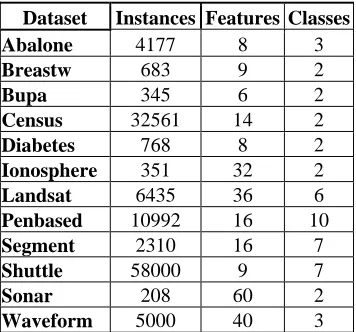
[image:3.612.354.532.73.239.2]In this section, we present experimental results on the performance of the proposed feature selection methods as well as comparisons with both the RELIEF and the SFS methods. Twelve well-known datasets from the Machine Learning Repository available at the University of California- Irvine are used in the experiments. A summary of these datasets is shown in table I. In the RELIEF, we have selected about 60% of the features in the dataset rather to use a threshold. The misclassification error rate of three classifiers, LDA, KNN y RPART is estimated after feature selection. In each experiment, we use 10-fold cross-validation to estimate the misclassification error.
Table I. Summary of the datasets used in this paper
Dataset Instances Features Classes
Abalone 4177 8 3
Breastw 683 9 2
Bupa 345 6 2
Census 32561 14 2
Diabetes 768 8 2
Ionosphere 351 32 2
Landsat 6435 36 6
Penbased 10992 16 10
Segment 2310 16 7
Shuttle 58000 9 7
Sonar 208 60 2
Waveform 5000 40 3
[image:3.612.322.565.416.653.2]Table II shows the misclassification error rates for the LDA classifier using the four selection methods. As a reference we have include also the misclassification error rate using all the features in each dataset. We can see that when the features are selected using the RELIEF then, the average of the misclassification error rate for all the datasets increases a 12% with respect to the one using all the features. The SFS shows a small increment of 1% whereas for the Wfeat this increment is about 7% and for the WfeatSFS increases in about 4%.
Table II. Misclassification error rate for the LDA classifier using the features selected by the four methods
Table III shows the misclassification error rates for the KNN classifier (We used k=3 neighbors for datasets having more than 5000 instances and k=5 neighbors, otherwise). We can see that when the RELIEF is used the average of the misclassification error rate for all the datasets increases in a 3% with respect to the one using all the features. On the other
Dataset All
features RELIEF SFS Wfeat WfeatSFS
Abalone 36.12 38.58 35.60 38.18 35.48
Breastw 4.00 4.80 3.69 4.83 4.16
Bupa 32.03 33.39 33.22 32.41 37.41
Census 17.51 18.67 17.45 17.57 17.46
Diabetes 22.99 32.84 23.46 23.13 23.23
Ionosphere 14.62 16.98 16.70 17.26 16.24
Landsat 16.07 16.41 16.42 17.15 17.61
Penbased 12.42 18.11 12.42 18.29 16.50
Segment 8.53 9.15 8.40 9.14 8.54
Shuttle 5.61 5.66 4.31 5.49 5.00
Sonar 25.29 26.63 25.38 25.96 22.60
Waveform 13.93 13.66 13.90 13.86 13.66
hand, after SFS the misclassification error rate decreases in a 10% whereas for the Wfeat this decrement is of 6% and for the WfeatSFS decreases in 10%.
Table III. Misclassification error rate for the KNN classifier using the features selected by the four methods
Table IV shows the misclassification error rates for the RPART classifier. After the RELIEF the average of the misclassification error rate for all datasets increases a 7% with respect to the one using all the features. After SFS there is a decrement of 6% whereas for the Wfeat increases in a 4%, and for the WfeatSFS decreases in 3.5%.
Table IV. Misclassification error rate for the RPART classifier using the features selected by the four methods.
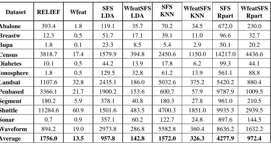
Table V shows a comparison of the computing running times for all the feature selection methods considered in this paper. As we can see the Wfeat is computed much faster than the
RELIEF. Also the WfeatSFS is computed, on average, three times much faster than the SFS for the three classifiers considered. Notice that the RELIEF performs badly for the Diabetes dataset when the three classifiers studied. Also, Penbased is a dataset that gives problems to all the feature selection methods except SFS.
The computer programs were written in C++ and R language, and are available upon request from the second author.
V. CONCLUSION
Our empirical results show that our filter method, Wfeat, outperforms the RELIEF in both the misclassification error rate and the speed of computation for the three classifiers considered in the paper. The gain in the computation time is quite evident. On the other hand, our proposed hybrid method, WfeatSFS, performs similarly to the wrapper method, SFS, regarding the misclassification error rate, for the three classifiers considered. But, the WfeatSFS is computed much faster than the SFS.
REFERENCES
[1] Blum, A. and Langley, P. Selection of relevant features and examples in machine learning. Artificial Intelligence, 1997, 97, 245-271. [2] Das, S. Filters, wrappers and a boosting-based hybrid for feature
selection. Proceedings of the Eighteenth International Conference on Machine Learning, 2001, pp. 74-81.
[3] Dash, M. and Liu, H. Feature selection for classifications. Intelligent Data Analysis: An International Journal,1997, 1, 131-156.
[4] Daza, A. Metodos para mejorar la calidad de un conjunto de datos para descubrir conocimiento. Doctoral Thesis Computing and Information Sciences and Engineering. University of Puerto Rico at Mayaguez, 2007.
[5] Guyon, I., and Elisseff, A. An introduction to variable and feature selection. Journal of Machine Learning Research, 2003, Vol 3 pp 1157-1182.
[6] Kim, W., Choi, B., Hong, E. and Lee, D. A taxonomy of dirty data. Data Mining and Knowledge Discovery, 2003, 7, 81-89.
[7] Kira, K. and Rendell, L. A. A practical approach to feature selection, Proceedings of the Ninth International Conference on Machine Learning, Aberdeen, Scotland, UK, Morgan Kaufmann Publishers, San Mateo, 1992, pp. 249–256.
[8] Kohavi, R. and John, G. Wrappers for feature subset selection. Artificial Intelligence, 1997, 97, 273-324.
[9] Kononenko, I. Estimating attributes: Analysis and extension of RELIEF. In: F. Bergadano and L. De Raedt, editors, Proceedings of the European Conference on Machine Learning, 1994, pp. 171-182, Catania, Italy. Berlin: Springer-Verlag.
[10] Liu, H. and Motoda, H. Feature Selection for Knowledge Discovery and Data Mining. 1998. Boston: Kluwer Academic Publishers. [11] Liu, H. y Setiono, R. Feature selection and classification - a
probabilistic wrapper approach. In Proc. 9th International Conference on Industrial & Engineering Applications of AI and Expert Systems, Fukuoka, Japan, 1996, pp. 419-424.
[12] Liu, H. and Yu, L. Toward integrating feature selection algorithms for classification and clustering, IEEE Transactions on Knowledge and Data Engineering, 2005, 17, 491-502
[13] Liu, H., Yu, L., Dash, M. and Motoda, H. Active feature selection using classes. Proceedings of the Seventh Pacific-Asia Conference on Knowledge Discovery and Data Mining, 2003, (PAKDD-03) pp. 474-485.
[14] Xing, E., Jordan, M. and Karp, R. Feature selection for high-dimensional genomic microarray data. Proceedings of the Eighteenth International Conference on Machine Learning, 2001, pp. 601-608.
Dataset All
features RELIEF SFS Wfeat WfeatSFS
Abalone 38.82 42.03 39.96 42.40 40.31
Breastw 3.19 4.10 3.09 3.34 3.02
Bupa 36.26 38.67 34.23 39.48 39.36
Census 24.89 19.89 22.81 15.78 17.24
Diabetes 30.48 39.30 26.64 28.49 26.98
Ionosphere 15.61 14.47 8.06 12.36 7.69
Landsat 8.95 9.74 9.40 9.63 9.95
Penbased 0.66 2.19 0.66 1.84 1.65
Segment 4.66 4.62 3.12 5.50 3.28
Shuttle 0.17 0.21 0.05 0.15 0.07
Sonar 18.61 18.65 18.56 15.96 17.40
Waveform 23.33 18.20 18.46 19.21 17.62
Average 17.14 17.67 15.42 16.18 15.38
Dataset All
features RELIEF SFS Wfeat WfeatSFS
Abalone 37.62 39.56 37.89 39.69 37.49
Breastw 5.42 4.80 4.56 5.07 4.56
Bupa 31.68 35.01 32.52 35.88 32.75
Census 15.91 18.51 15.43 15.93 15.43
Diabetes 25.96 33.42 25.26 26.93 25.73
Ionosphere 12.39 11.40 10.20 11.62 9.86
Landsat 18.66 19.02 18.39 19.06 18.74
Penbased 18.21 19.99 16.81 20.10 19.61
Segment 8.31 8.26 8.02 8.37 8.37
Shuttle 0.53 0.53 0.53 0.53 0.53
Sonar 28.75 28.41 21.34 29.23 25.10
Waveform 26.63 26.92 26.00 26.84 26.38
[15] Yang, Y. and Pederson, J. 7 A comparative study on feature selection in text categorization. Proceedings of the 14th International Conference on Machine Learning, 1997, pp. 412–420.
[16] Yu, L. and Liu, H. Efficiently handling feature redundancy in high-dimensional data. Conference on Knowledge Discovery in Data. Proceedings of the ninth ACM SIGKDD international conference on Knowledge discovery and data mining. Washington, D.C. KDD, 2003, pp. 685-690.
[image:5.612.92.524.233.463.2][17] Zhu, X., Wu, X. y Chen, Q. Eliminating class noise in large datasets. Proceedings of the 20th ICML International Conference on Machine Learning (ICML 2003). Washington D.C., 2003, pp. 920-927.
Table V. Computation time (secs.) for the four feature selection methods including the wrappers with the three classifiers
Dataset RELIEF Wfeat SFS
LDA
WfeatSFS LDA
SFS
KNN WfeatSFSKNN Rpart SFS WfeatSFSRpart
Abalone 393.4 1.8 119.1 35.7 70.2 34.5 672.0 230.0
Breastw 12.3 0.5 51.7 17.1 39.1 11.0 96.6 32.7
Bupa 1.8 0.1 23.3 8.5 5.4 2.9 50.1 20.2
Census 3818.7 17.4 1579.9 394.8 2450.6 1150.0 14217.0 4436.6
Diabetes 10.1 0.5 44.2 13.9 17.8 6.2 99.3 44.1
Ionosphere 1.8 0.5 129.5 32.8 61.2 13.9 561.1 88.8
Landsat 1107.6 32.8 2435.1 186.0 5032.6 375.2 5420.2 880.4
Penbased 3366.1 21.7 1900.2 153.6 600.7 57.9 9787.9 1009.5
Segment 180.2 5.9 378.1 40.8 180.3 27.8 961.0 210.5
Shuttle 11284.6 60.9 1501.6 483.5 4700.3 1851.0 9935.3 2939.5
Sonar 0.7 0.9 357.1 60.2 122.7 24.8 897.6 144.5
Waveform 894.2 19.0 2973.8 286.8 5582.8 360.4 8636.2 1632.2